1. Introduction
Speech recognition systems allow computers to process audio signals into text or perform specific tasks. Highly developed speech recognition systems will allow you to change the way you communicate with a computer. The possibilities seem limitless—from simply giving commands to the machine (so-called hands-free computing), by dictating text and automatic writing, to the possibility of voice control of devices installed in our homes. Another very important application will probably be the development of security systems based on user speech recognition. The human voice is as unique as fingerprints and can therefore be a very practical tool, e.g., for controlling access to guarded objects. Another application will be the ability to translate computer speech in real time online. Combining speech recognition with a mechanism that translates recognized content into other languages would completely revolutionize intercultural communication. A public real-time translation system used, e.g., in Skype technology, would give average users unlimited communication possibilities and lead to the creation of a real global village. A language barrier would be overcome. Such a system would give people access to countless sources of information in foreign language versions [
1,
2,
3,
4].
Audio coding is a major problem in speech recognition. It is a technique for representing a digital signal in the form of information bits. Due to the high interest in coding on the part of industry, research on speech coding methods is very popular among researchers. Standardization organizations are working to introduce global coding norms and standards. Thanks to them, the industry will be able to meet the market demand for speech processing products [
1,
2].
Modern speech recognition systems use deep learning techniques [
5,
6,
7]. They are used to represent features and to model the language [
8,
9].
In classification tasks, deep neural networks (DNN) are used, among others, with polynomial logistic regression, as well as by introducing modifications using support vector machines (SVM) [
10,
11]. Better results are achieved by the recently popular convolution neural networks [
12,
13].
New frameworks are being created for the fastest open-source deep learning speech recognition framework [
14]. Work is underway to improve their efficiency compared to existing ones such as ESPNet, Kaldi, and OpenSeq2Seq.
There are also solutions in which the architecture of the Recurrent Neural Network (RNN) is used to obtain lightweight and high accuracy models that can run locally [
15]. This will allow the use in real time.
There are works on algorithms implemented in the frequency domain that allow speech analysis by identifying the intended fundamental frequency of the human voice, even in the presence of subharmonics [
16].
The problem is also examined covered in audio recognition to the better-studied domain of image classification, where the powerful techniques of convolutional neural networks are fully developed [
17].
The article presents the use of convolutional neural networks to recognize continuous speech and isolated words. As part of our research, we’ve developed speech sharing algorithms and speech coding algorithms using RGB (Red, Green, Blue) images. It can be used for a symmetrical stereo signal. Our method uses a convolution of three techniques (mel-frequency cepstral coefficients (MFCC), time and spectrum) in contrast to the similar method [
18] that uses convolution of only two components (time and spectrum).
2. Convolutional Neural Networks
The structure of the visual cortex in mammalian brains was a pattern for creating the Convolutional Neural Network (CNN) [
19]. The local pixel arrangement determines the recognition of the shape of the object, so CNN begins to analyse the image with smaller local patterns, and then combines them into more complex shapes. The effectiveness of CNN in recognizing objects in images can be the basis for solving the problem of speech recognition. There is a picture at CNN and its architecture reflects this. Thus, our method uses sound encoding using images. A typical CNN network includes convolution layers, pooling layers, and fully connected layers. Convolution layers and pooling layers constitute internal structure, and fully connected layers are responsible for generating class probability.
2.1. Convolutional Layer
Convolutional layer (CL) consists of neurons connected to the receptive field of the previous layer. The neurons in the same feature map share the same weights [
20]. CL contains a set of learnable filters. One filter activates when a specific shape or blob of colour occurs within a local area [
20]. Each CL has multiple filters, while the filter is a set of learnable weights corresponding to the neurons in the previous layer. The filter is small spatially (usual filter sizes are 3 × 3, 5 × 5 or less frequently 7 × 7) and extends along the full depth of the previous layer.
The depth of CL depends on the number of various functions used in the image that are obtained by the number of learnable filters. Every neuron in CL uses weights of exactly one CL’s filter; many neurons use the same weights. The neurons in CL are segmented into feature maps by the filter they are using. The receptive field of a neuron in CL specifies the local area of the neuron’s connectivity onto the previous layer. All neurons within the same CL have the same size of their receptive fields. All connections of a given neuron form the reception field of this neuron. The volume of the receptive field is always equal to the filter size of a particular CL multiplied by the depth of previous layer.
The activation is computed by application of the activation function over the potential. As an activation function, most of the time, the ramp function is used—also referred as the ReLU unit. If the specific feature matters in one part of the image, usually the feature is important also in the rest of the image. One of the most important hyper-parameters next to the number of filters is stride. When determining the stride, take into account the size of the receptive field of a neuron and the size of the image. In case it is incorrectly chosen, the stride must be changed or zero-padding should be used, in order to keep a specific input size, or to normalize images with various shapes.
2.2. Pooling Layer
Pooling layer (PL) is an effective way of nonlinear down-sampling. It has as the CL receptive field and stride; however, it is not adding any learnable parameters. PL is usually put after the CL. The receptive field of neuron in PL is two-dimensional. Max-PL is the most frequently used PL. Each neuron outputs the maximum of its receptive field. Usually, the stride is the same as the size of the receptive field. The receptive fields do not overlap but touch. In most cases, stride and size of receptive field are 2 × 2. Max-PL amplifies the most present feature (pattern) of its receptive field and throws away the rest. The intuition is that, once a feature has been found, its rough location relative to other features is more important than its exact location. The PL is effectively reducing the spatial size of the representation and does not add any new parameters—reducing them for latter layers, making the computation more feasible.
Due to its destructiveness—throwing away 75% of input information in case of a small 2 × 2 receptive field—the current trend prefers stacked CLs eventually with
stride and uses PLs very occasionally or discards them altogether [
21].
2.3. Structure
As a feed-forward artificial neural network, the CNN consists of neurons with learnable weights and biases. CNN’s neurons still contains activation function and the whole network expresses single differentiable score function. The position of the pixel matters in comparison with MLP. It receives three-dimensional space input ()—the value of the z-th channel of the pixel or occurrence of z-th feature of CL at position ().
The CL and PL are locally connected to the outputs of the previous layer, recognizing or magnifying local patterns in the image. PL is usually put after the CL. This pair of layers is repeatedly stacked upon each other following with the fully connected layers (FC) at the top. The positions of neurons in the previous layer are always considered without stride as inputs for latter layers. The FC is connected to all outputs of the last PL. The outputs of the last PL should already represent complex structures and shapes. The FC follows usually with another one or two layers finally outputting the class scores.
The usual architecture can be: input layer (IL), CL, PL, CL, PL, FC, FC. Recent studies suggest stacking many CLs together with fewer PLs.
2.4. Back-Propagation
The single evaluation is completely consistent with the feed-forward neural network. The input data or activations are passed to the next layers, the dot product is computed over which activation function is applied. Down-sampling the network using PL might be present. At the end, two or three fully connected layers are stacked. In order to use the gradient descent learning algorithm, the gradient must be computed.
The usual back-propagation algorithm is applied with two technical updates. The classical back-propagation algorithm would calculate different partial derivatives of weights belonging to the neurons in the same filter; however, these must stay the same. Therefore, derivatives of loss function with respect to weights of neurons belonging to the same feature map are added up together.
The update of back-propagation itself is when dealing with -PLs. The back propagating error is routed only to those neurons that have not been filtered with max-pooling. It is usual to track indices of kept neurons during forward propagation to speed up the back-propagation.
3. Deep Autoencoder
3.1. Autoencoder
Autoencoder is a feed-forward neural network where expected output is equal to the input of the network—its goal is to reconstruct its own inputs. Therefore, autoencoders are belonging to the group of unsupervised learning models [
19]. Usually, the autoencoder consists of an IL
of one or many hidden layers
and output layer lk. Since the idea of autoencoders is very similar to the Restricted-Boltzman Machine, it is common for the structure of autoencoders to follow the rule
. Each autoencoder consists of an encoder and decoder.
The encoder can be used for compression. Unlike Principal Component Analysis (PCA) analysis restricted to linear mapping, the encoder represents nonlinear richer underlying structures of the data [
22]. The activations of the
layer can be further used for classification. FCs are appended with the size of the last corresponding to the number of labels. The usual learning algorithms are used.
3.2. Deep Autoencoder
A Deep Autoencoder consists of many layers stacked on each other allowing to discover more complicated and nonlinear structures of the data. Since it may be complicated to tune deep autoencoder networks, commonly the training procedure is made of two steps:
Pre-training; each layer is pre-trained. Firstly, the pair l0 as an example and as an encoder is used. The goal is to find representation of in using the right optimizer. The weights to and to may be tied up representing the Restricted Boltzman-Machine. When good representation of inputs is encoded in , the pair is pre-trained further until pair is reached.
Fine-tuning, the full network is connected and fine-tuned. In case of classification, the encodings of input data points can be used for classification training or the whole network.
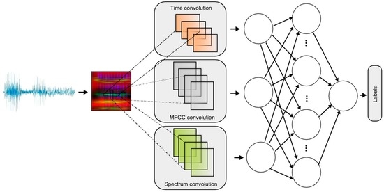
4. Time Frequency Convolution
Thus far, the CNNs used for speech recognition have been built based on frequency. CNNs using the convolution spectrum could also be found. In this article, we present the applied CNN. As shown in
Figure 1, a convolution of three CLs was used. An important novelty in the discussed network is conducting the convolution taking into account time (Time convolution) and frequency (MFCC convolution and Spectrum convolution). The use of time convolution helps reduce problems with time artifacts, whereas the problem of small spectral shifts (e.g., different lengths of vocal paths in loudspeakers) is solved by using across frequency. In addition, the MFCC convolution introduced reduces noise sensitivity. MFCC allows you to adapt the frequency analysis to the method of analysis used by the human ear. The spectrum analyses the signal linearly, while the MFCC performs linear analysis to a frequency of 1 kHz, and the 1 kHz above characteristic becomes exponential.
To encode the sounds using the RGB image, the MFCC coefficients [
23,
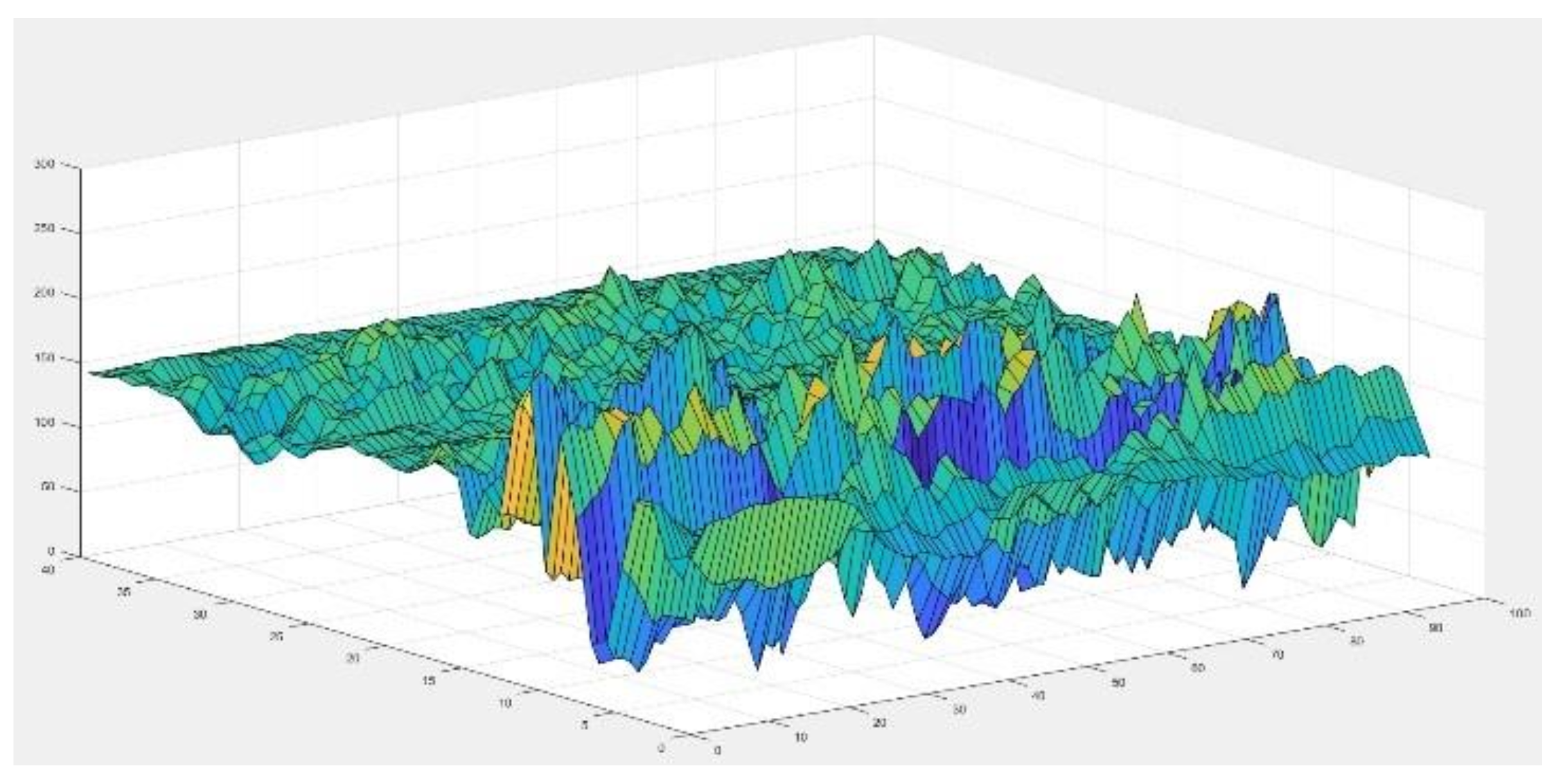
24] for the R component were applied, the time characteristic was used for the G component, and the signal source was used for the B component. Convolution of the three components R, G and B is performed in parallel. Coefficient maps, accepted for coding, had different sizes. Of course, in order to create a colour image, it was necessary to scale the RGB components to one size. It was assumed that individual sounds will be coded using images with a size of 120 × 120 pixels. The time characteristics for the word “
seven” are shown in
Figure 2.
Examples of characteristics for the word “
seven” are shown in
Figure 3,
Figure 4 and
Figure 5. Parameters of the coefficient maps were chosen in an experimental way. The accepted criterion was the best initial adjustment to the size of 120 × 120 pixels.
For such defined RGB components, it was possible to create an RGB image, which is a visual pattern for sound. It was assumed that each syllable should be coded separately. Of course, it is possible to encode combined phonemes that do not always form a syllable, but are, for example, combined with silence. In the example recording for the word “
seven”, the algorithm generated the division “
se”–“
ven”. An example of the coded syllable “
se” and “
ven” is shown in
Figure 6.
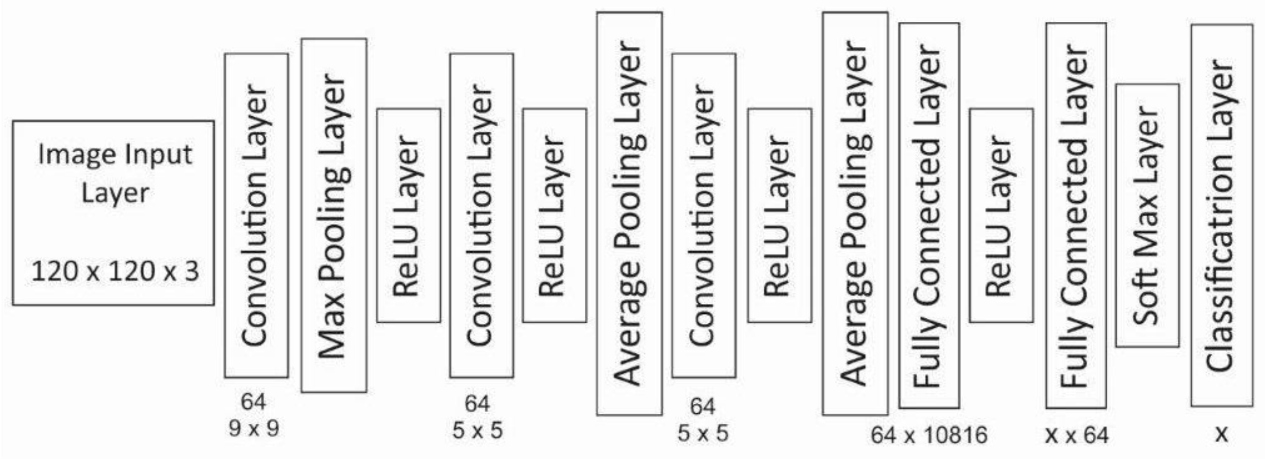
5. Neural Network Structure
The proposed CNN consisted of 15 layers. The first CL contained 64 filters with dimensions of 9 × 9. Three CLs are responsible for coding information, transferred into two FCs. The network diagram is shown in
Figure 12.
The last layer (FC) and Classification Layer contains X possible outputs. X depends on the training data set. The input data are either an isolated word or a syllable. For isolated words, X is the number of recognized words. For syllables, X is the number of different syllables determined from the training data. Sometimes, it happens that the split algorithm also combines individual sounds with silence.
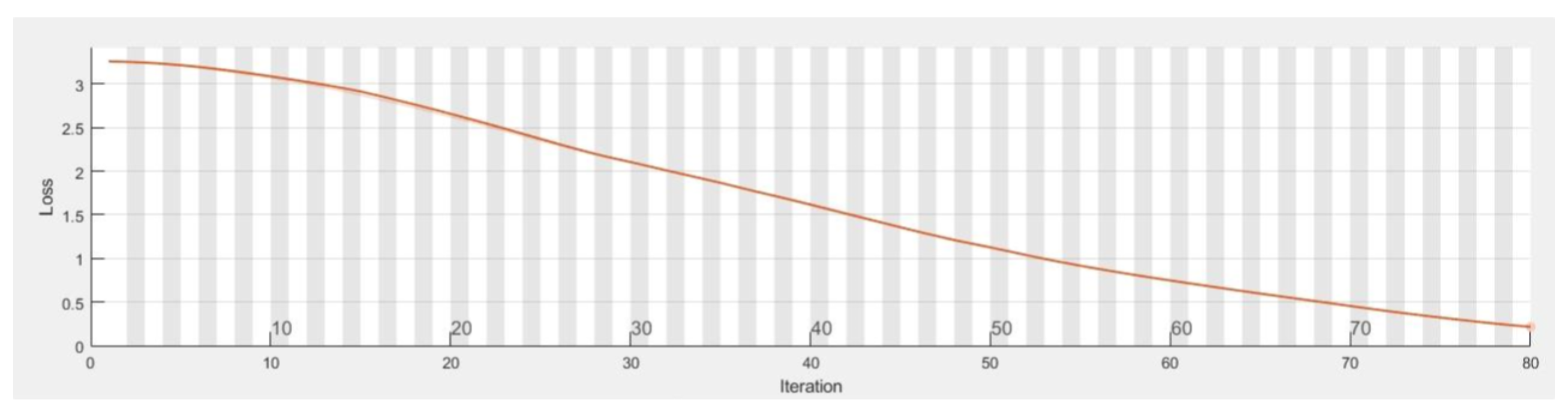
Figure 13 and
Figure 14 show training metrics at every iteration. Each iteration is an estimation of the gradient and an update of the network parameters.
6. Results and Discussion
The studies included two important issues. The first concerned the correctness of the work of the algorithm, realizing the division of speech into syllables. A method was applied that takes into account signal energy and signal frequency for the stationary fragment under consideration. The division into individual syllables was made for the experimentally selected threshold values. For each isolated syllable (which could also include silence), the image was created as a graphic pattern. Each syllable pattern has been saved as an image in a directory name corresponding to the designated syllable. The experiment was carried out for insulated words and continuous speech. A different number of words have been adopted for continuous speech.
Table 1 shows the results of an experiment concerning the division into syllables. The research was conducted on our own database and public audio books.
The most common in the literature are works that use time and frequency characteristics for analysis. Our work includes a new component in MFCC signal analysis. The advantage of this technique is to include sound analysis just like the human ear.
The obtained result is difficult to compare to other existing methods because the previous approaches included only one or two components (time and spectrum). In addition, these methods were used for grayscale images, while our method uses ternary analysis (in addition MFCC) for RGB images.
As expected, the best results were obtained for the separated words—98%. It is obvious that the results obtained for continuous speech have a lower recognition rate. Nevertheless, the result of 70–80% is satisfactory.
The second type of research concerned the evaluation of the effectiveness of speech recognition for isolated words and for continuous speech. The recorded data were divided into training data and test data, at a ratio of 70 to 30. The learning time of the neural network and the number of epochs required for correct learning were also examined. The results of the main experiment are shown in
Table 2.
Based on the results shown in
Table 2, it can be seen that continuous speech recognition is a much more difficult task. The improvement of this factor will be the subject of further work of our team.
7. Conclusions
Research has shown that effective speech recognition is possible for isolated words. Appropriate speech coding by means of images allows use in CNNs. The proposed method of speech coding is an interesting alternative to the classic approach. It has been noticed that, when speaking slowly, the division into syllables is quite easy. Further work will focus on increasing the efficiency of word recognition through a more accurate division into syllables. The algorithm MFCC should also be developed further, as it introduced the biggest mistakes in the visual coding of speech. This method can be used for symmetrical stereo sound. We also want to refine the division of speech into syllables, by introducing better divisions. This will allow for the smooth creation of learning data, which in its current form was the most difficult task.
Author Contributions
M.K. devised the method and guided the whole process to create this paper; J.B., J.K. and M.K. implemented the method and performed the experiments; M.K. and J.K. wrote the paper.
Funding
This project was financed under the program of the Minister of Science and Higher Education under the name “Regional Initiative of Excellence” in the years 2019–2022 project number 020/RID/2018/19, and the amount of financing is 12,000,000 PLN.
Conflicts of Interest
The authors declare no conflict of interest.
References
- Riccardi, G.; Hakkani-Tur, D. Active learning: Theory and applications to automatic speech recognition. IEEE Trans. Speech Andaudio Process. 2005, 13, 504–511. [Google Scholar] [CrossRef]
- Xiong, W.; Wu, L.; Alleva, F.; Droppo, J.; Huang, X.; Stolcke, A. The Microsoft 2017 Conversational Speech Recognition System. In Proceedings of the 2018 IEEE International Conference on Acoustics, Speech and Signal Processing (ICASSP), Calgary, AB, Canada, 15–20 April 2018. [Google Scholar]
- Wessel, F.; Ney, H. Unsupervised training of acoustic models for large vocabulary continuous speech recognition. IEEE Trans. Speech Audio Process. 2005, 13, 23–31. [Google Scholar] [CrossRef]
- Windmann, S.; Haeb-Umbach, R. Approaches to Iterative Speech Feature Enhancement and Recognition. IEEE Trans. Audio Speech Lang. Process. 2009, 17, 974–984. [Google Scholar] [CrossRef] [Green Version]
- Mohamed, A.R.; Dahl, G.E.; Hinton, G.E. Acoustic Modeling Using Deep Belief Networks. IEEE Trans. Audio Speech Lang. Process. 2012, 20, 14–22. [Google Scholar] [CrossRef]
- Mitra, V.; Franco, H. Time-frequency convolutional networks for robust speech recognition. In Proceedings of the 2015 IEEE Workshop on Automatic Speech Recognition and Understanding (ASRU), Scottsdale, AZ, USA, 13–17 December 2015; pp. 317–323. [Google Scholar]
- Yu, D.; Seide, F.; Li, G. Conversational Speech Transcription Using Context-Dependent Deep Neural Networks. In Proceedings of the 12th Annual Conference of the International Speech Communication Association, Florence, Italy, 27–31 August 2011. [Google Scholar]
- Tüske, Z.; Golik, P.; Schlüter, R. Acoustic modeling with deep neural networks using raw time signal for LVCSR. In Proceedings of the 15th Annual Conference of the International Speech Communication Association, Singapore, 14–18 September 2014. [Google Scholar]
- Arisoy, E.; Sainath, T.N.; Kingsbury, B.; Ramabhadran, B. Deep Neural Network Language Models. In Proceedings of the NAACL-HLT 2012 Workshop: Will We Ever Really Replace the N-gram Model? On the Future of Language Modeling for HLT; Association for Computational Linguistics: Montréal, QC, Canada, 2012; pp. 20–28. [Google Scholar]
- Lekshmi, K.R.; Sherly, D.E. Automatic Speech Recognition using different Neural Network Architectures—A Survey. Int. J. Comput. Sci. Inf. Technol. 2016, 7, 2422–2427. [Google Scholar]
- Zhang, S.-X.; Liu, C.; Yao, K.; Gong, Y. Deep neural support vector machines for speech recognition. In Proceedings of the 2015 IEEE International Conference on Acoustics, Speech and Signal Processing (ICASSP), South Brisbane, Queensland, Australia, 19–24 April 2015; pp. 4275–4279. [Google Scholar]
- Sainath, T.N.; Mohamed, A.R.; Kingsbury, B.; Ramabhadran, B. Deep convolutional neural networks for LVCSR. In Proceedings of the 2013 IEEE International Conference on Acoustics, Speech and Signal Processing, Vancouver, BC, Canada, 26–31 May 2013; pp. 8614–8618. [Google Scholar]
- Mitra, V.; Wang, W.; Franco, H.; Lei, Y.; Bartels, C.; Graciarena, M. Evaluating robust features on deep neural networks for speech recognition in noisy and channel mismatched conditions. In Proceedings of the Fifteenth Annual Conference of the International Speech Communication Association, Singapore, 14–18 September 2014. [Google Scholar]
- Pratap, V.; Hannun, A.; Xu, Q.; Cai, J.; Kahn, J.; Synnaeve, G.; Liptchinsky, V.; Collobert, R. wav2letter++: The Fastest Open-source Speech Recognition System. arXiv 2018, arXiv:1812.07625. [Google Scholar]
- de Andrade, D.C. Recognizing Speech Commands Using Recurrent Neural Networks with Attention. Available online: https://towardsdatascience.com/recognizing-speech-commands-using-recurrent-neural-networks-with-attention-c2b2ba17c837 (accessed on 27 December 2018).
- Andrade, D.C.; Trabasso, L.G.; Oliveira, D.S.F. RA Robust Frequency-Domain Method For Estimation of Intended Fundamental Frequency In Voice Analysis. Int. J. Innov. Sci. Res. 2018, 7, 1257–1263. [Google Scholar]
- Krishna Gouda, S.; Kanetkar, S.; Harrison, D.; Warmuth, M.K. Speech Recognition: Keyword Spotting Through Image Recognition. arXiv 2018, arXiv:1803.03759. [Google Scholar]
- Abdel-Hamid, O.; Deng, L.; Yu, D. Exploring Convolutional Neural Network Structures and Optimization Techniques for Speech Recognition. In Interspeech 2013; ISCA: Singapore, 2013. [Google Scholar]
- Rawat, W.; Wang, Z. Deep Convolutional Neural Networks for Image Classification: A Comprehensive Review. Neural Comput. 2017, 29, 2352–2449. [Google Scholar] [CrossRef] [PubMed]
- Bengio, Y. Learning Deep Architectures for AI. Found. Trends® Mach. Learn. 2009, 2, 1–127. [Google Scholar] [CrossRef]
- He, K.; Zhang, X.; Ren, S.; Sun, J. Deep Residual Learning for Image Recognition. In Proceedings of the IEEE Conference on Computer Vision and Pattern Recognition (CVPR), Las Vegas, NV, USA, 27–30 June 2016. [Google Scholar]
- Hinton, G.E.; Salakhutdinov, R.R. Reducing the dimensionality of data with neural networks. Sci. Am. Assoc. Adv. Sci. 2006, 313, 504–507. [Google Scholar] [CrossRef] [PubMed]
- Kubanek, M.; Bobulski, J.; Adrjanowicz, L. Characteristics of the use of coupled hidden Markov models for audio-visual polish speech recognition. Bull. Pol. Acad. Sci. Tech. Sci. 2012, 60, 307–316. [Google Scholar] [CrossRef]
- Kubanek, M.; Rydzek, S. A Hybrid Method of User Identification with Use Independent Speech and Facial Asymmetry. In Proceedings of the 9th International Conference on Artificial Intelligence and Soft Computing (ICAISC 2008), Zakopane, Poland, 22–26 June 2008; Springer: Berlin/Heildelberg, Germany, 2008; pp. 818–827. [Google Scholar]
© 2019 by the authors. Licensee MDPI, Basel, Switzerland. This article is an open access article distributed under the terms and conditions of the Creative Commons Attribution (CC BY) license (http://creativecommons.org/licenses/by/4.0/).


