Quantile-Based Estimation of the Finite Cauchy Mixture Model

Abstract

Heterogeneity and outliers are two aspects which add considerable complexity to the analysis of data. The Cauchy mixture model is an attractive device to deal with both issues simultaneously. This paper develops an Expectation-Maximization-type algorithm to estimate the Cauchy mixture parameters. The main ingredient of the algorithm are appropriately weighted component-wise quantiles which can be efficiently computed. The effectiveness of the method is demonstrated through a simulation study, and the techniques are illustrated by real data from the fields of psychology, engineering and computer vision.

1. Introduction

Recently, many works on finite mixture models have been produced which support researchers in modelling and interpreting data stemming from unobserved (“latent”) sub-populations. Finite mixture models can handle heterogeneous data by providing a flexible representation in the form of a weighted sum of probability densities. Applications of such models include clustering, classification and data visualization, but mixture models are also used for simulation steps within evolutionary algorithms, or as a building block of advanced statistical models (for instance, multi-level models) in order to adequately account for the error structure of the problem at hand. Mixture models have furthermore been used as a tool to address over-dispersion, which in turn is related to the presence of long-tailed distributions. Examples for data situations which possess a mixture structure include industrial measurements of a certain quantity which, during the measurement process, underwent a slight, possibly unnoted, change of conditions. An explicit example within an industrial context, involving temperature measurements from a glass melter, is provided below.

A well-known problem with the typically employed Gaussian mixtures is that these are not able to deal well with outlying observations. If the Gaussian mixture components are allowed to have unequal variances, it has frequently been observed that specific outlying observations “capture” a mixture component for their own, which will be centered at that outlier and will approach zero variance as the expectation-maximization routine progresses [1]. Since “zero variance” corresponds to “infinite likelihood” in the context of Gaussian distributions, one also talks here of likelihood spikes. Several methods have been proposed to deal with this problem in the literature, including the use of “smoothed” variances [1], the use of a mixtures with an “improper” component which mops up the outliers [2], and the use of mixtures of distributions with thicker tails, such as t-distributions [3].

However, these existing techniques come with some limitations. The first two approaches stabilize the estimation numerically, but, in doing so, they dismiss the possibility of the outliers actually being a genuine feature of some physically meaningful component, even if strongly outlying. In the third approach, one considers, for some univariate and i.i.d. response data $x_1,\dots ,x_n$ a mixture of $K\ge 2$ t-distributions, where each of the means, variances and degrees of freedom can be estimated from the data.

Fitting mixtures of t-distributions is conceptually and computationally demanding, and it was left open by Peel et al. [3] how stable this procedure behaves when the degrees of freedom, q, approach the value 1. This limiting case, at $q=1$, defines the $t\left(1\right)$ distribution, also known as a Cauchy distribution. The Cauchy and Gaussian models can be seen as opposite ends of the spectrum of possible $t\left(q\right)$ distributions, ranging from $t\left(1\right)$ to $t(\infty )$, respectively. Hence, this manuscript aims to complete this spectrum by proposing a mixture of Cauchy distributions.

The Cauchy distribution has several interesting properties. While being a symmetric distribution, its mean does not exist. The Cauchy distribution is well known for its propensity to produce massive outliers [4] and hence can deal with observations which might be considered unreasonable or pathological. Interestingly, such outliers, which may (or may not) materialize on either side of the distribution, with potentially wildly varying degree of outlyingness, can break the symmetry of the observed data, despite the symmetry property of their generating distribution. Allowing additionally for heterogeneity of location parameters through a mixture model, as motivated above, enables the data analyst to deal with highly asymmetric data patterns.

Asymmetry is a fundamental problem in financial and economic data modeling. Many papers have suggested approaches for capturing asymmetry in financial data. An ensemble system based on neural networks to predict intraday volatility is presented in [5]. A comparison of centrality metrics’ performance on stock market datasets was made in [6]. The asymmetric impact of prices and volatilities of gold and oil on emerging markets was considered in [7]. However, all of these approaches focus on certain notions of skewness or (non-)centrality to describe asymmetry, rather than accounting for outliers and heterogeneity explicitly through a mixture model as considered herein.

Mixture models are typically estimated through the Expectation-Maximization (EM) algorithm, which alternates between an E-step, in which one calculates, for each observation, probabilities of component membership, and an M-step, which maximizes an expected “complete” likelihood where these membership probabilities are assumed as fixed. This amounts, effectively, to the problem of maximizing a weighted version of the single-distribution likelihood. However, in the Cauchy case, this is not a trivial task. Even for the plain Cauchy model, the maximum likelihood estimator of the location parameter does usually not exist in analytical form, and, what is worse, the log likelihood itself suffers from the existence of inconsistent local maxima [8]. However, it is well known that Cauchy parameters can be easily estimated through empirical quantiles of the data. The main objective of this paper is to investigate how this approach can be extended in order to fit Cauchy mixtures; using appropriately weighted quantiles in the Maximization step. It should be stated already now that, by following this line of thought, the resulting methodology will not constitute an EM-algorithm in the strict sense of its definition, and will not inherit its theoretical properties. Therefore, we use the weaker terminology EM-type to refer to this algorithm henceforth.

Of course, mixture models can also be used in conjunction with many other, discrete or continuous, or even mixed, distributions. More than half a century ago, foundations for estimating an extensive class of mixture models were laid by Boes [9]. McLachlan and Peel [10] presented a comprehensive account of finite mixture models and their properties. Contributions for specific distributions include, without claiming completeness, the work by Zhang et al. [11] who studied a finite mixture Weibull distribution with two components to describe tree diameters for forest data, and Zaman et al. [12] who studied chi-squared mixtures of the gamma distribution. Suksaengrakcharoen and Bodhisuwan [13] proposed a mixture of generalized gamma and length biased generalized gamma distributions. Karim et al. [14] studied mixtures of Rayleigh distributions by assuming that the weight functions follow chi-square, t and F sampling distributions. Sindhu and Feroze [15] discussed parameter estimation of the Rayleigh mixture model using Bayesian methods. Applications of the mixture model are found in the environmental and natural sciences, education, psychology, business, and other fields.

This paper is organized as follows. In Section 2, we discuss some preliminaries; specifically, in Section 2.1, we explain the general concept of mixture models and the EM algorithm, and, in Section 2.2, we recall the definition and properties of the Cauchy distribution. In Section 3, we estimate the parameters of a Cauchy mixture model by applying an EM-type algorithm. The effectiveness of the proposed model is then demonstrated through simulated (Section 4) and real data (Section 5). In the last section, we contribute some remarks and present a conclusion.

2. Preliminaries

2.1. Mixture Models

Consider independent one-dimensional values $x_i$, $i=1,\dots ,n$ forming a dataset $D=\{x_1,x_2,\cdots ,x_n\}$. We are interested in situations in which it is plausible to assume that all elements of D have been generated by the same univariate density function $f(·|\theta )$, albeit, due to hetereogeneity, with different settings of $\theta \in {\mathbb{R}}^m$. More specifically, one assumes that only a set of K (unknown) parameter settings ${\theta }_j$, $j=1,\dots ,K$, each of which associated with some subpopulation proportion $p_j$, is responsible for the creation of the data. This situation is then described by a finite mixture model with K components,

$$f\left(x\right|\Theta )=\sum _{j=1}^K{p}_{j}f\left(x\right|{\theta }_j),$$

(1)

where the $p_j$ are the mixture weights, which represent the probability that x is generated by component j, with ${\sum }_{j=1}^K{p}_j=1$. That is, the parameter space of the mixture model in Equation (1) can be summarized by $\Theta =\{p_1,\cdots ,p_{K-1},{\theta }_1,\cdots ,{\theta }_K\}$ with cardinality $N_{\theta }=K(m+1)-1$.

For later use, denote by $z_{ij}$ an indicator which takes the value 1 if case i belongs to component j (or, more precisely, is “generated” from the random variable which represents component j). Then, one finds through a direct application of Bayes Rule

$$w_{ij}\equiv P(z_{ij}=1|x_i,\Theta )=\frac{p_{j}f\left(x_i\right|{\theta }_j)}{{\sum }_{m=1}^K{p}_{m}f\left(x_i\right|{\theta }_m)},i=1,\cdots ,n,j=1,\cdots ,K.$$

(2)

These membership weights, sometimes also called “responsibilities”, play an important role for mixture models. Firstly, they constitute the E-step of the EM algorithm, in which the probabilities of class membership are updated given the current parameter estimates; and, secondly, after convergence of that algorithm, they deliver a weight matrix $W={\left(w_{ij}\right)}_{1\le i\le n,1\le j\le K}$, which can be seen as a “final verdict” to which class each observations belongs, and can be used for clustering and classification purposes.

Mixture models are most commonly estimated through maximum likelihood estimation, which is, conceptually, not straightforward since the likelihood

$$L(\Theta )=\prod _{i=1}^{n}f\left(x_i\right|\Theta )=\prod _{i=1}^n\left(\sum _{j=1}^K{p}_{j}f\left(x_i\right|{\theta }_j)\right)$$

(3)

does not allow for an analytical maximization. A widely used solution to this problem is given by the Expectation-Maximization (EM) algorithm, which exploits the property that, given the $w_{ij}$, estimation of model parameters can usually be carried out as a simple weighted version of the corresponding one-component problem. This solution constitutes the M-step of the algorithm, and can be formally described as the maximization of the expectation of the complete likelihood, that is the augmented likelihood function assuming all $w_{ij}$ as known. Hence, one can estimate $\Theta$ by iterating, starting from some value ${\Theta }_0$, between the E-step and the M-step.

We omit further detail on the general properties of this algorithm as this has been covered in abundance elsewhere [1,10], but we provide the adapted steps in the context of the Cauchy model in explicit form in Section 3.

2.2. Cauchy Distribution

A random variable X has a Cauchy distribution with location parameter $\alpha \in \mathbb{R}$ and scale parameter $\gamma >0$, if its probability mass function takes the shape

$$f\left(x\right|\alpha ,\gamma )=\frac{1}{\pi \gamma \left[1+{\left(\frac{x-\alpha }{\gamma }\right)}^2\right]},-\infty <x<\infty .$$

(4)

This entails the cumulative distribution function,

$$F\left(x\right|\alpha ,\gamma )=\frac{1}{2}+\frac{1}{\pi }arctan\frac{x-\alpha }{\gamma },-\infty <x<\infty ,$$

(5)

and corresponding quantile function,

$$q\left(c\right|\alpha ,\gamma )=\alpha +\gamma tan\left[\pi \left(c-\frac{1}{2}\right)\right],$$

(6)

where c is a given percentile, which then clearly implies $(q\circ F)\left(x\right)=x$.

The Cauchy distribution is a unimodal and symmetric distribution, with the maximum density attained for $x=\alpha$ with $f\left(\alpha \right|\alpha ,\gamma )=\frac{1}{\pi \gamma }$. The mean and the variance of the Cauchy distribution are undefined, and the distribution does not have finite moments [16,17]. Since both the mode and the median of the Cauchy distribution coincide with $\alpha$ (the latter being immediately clear from Equation (6) by setting $c=1/2$), the sample mode and the sample median are the most natural candidates for the task of location estimation. Since the sample mode is not necessarily easy to estimate, the sample median

$$\widehat{\alpha }=\mathrm{Med}(x_1,\dots ,x_n)=\underset{x}{min}\{F_n\left(x\right)\ge 0.5\}$$

(7)

where $F_n\left(x\right)=\frac{1}{n}{\sum }_{i=1}^n\mathbf{1}\{x_i\le x\}$, appears favorable. Concerning the estimation of $\gamma$, note that again from Equation (6) one has

$$q(3/4|\alpha ,\gamma )-q(1/4|\alpha ,\gamma )=2\gamma$$

so that

$$\widehat{\gamma }=\frac{1}{2}IQR(x_1,\dots ,x_n),$$

(8)

where IQR denotes the empirical interquartile range, is a suitable estimator of $\gamma$.

An appealing property of the estimators in Equations (7) and (8) is their simplicity, being based only on three easily computable quantiles of the data. It has been argued in the literature already many decades ago that more efficient estimators of the Cauchy location parameter should be used, such as a weighted averages of several, symmetrically weighted, quantiles [18], a linear combination of order statistics [19], or a suitably trimmed mean [20]. In addition, Tiku [21] proposed an estimator based on “Modified Maximum Likelihood” (MML), which is conceptually simple, but practically difficult to implement, especially with view to the mixture scenario that we have in mind.

In light of such considerations, we assessed the performance of Equations (7) and (8) in a short simulation study. We are particularly interested in the closeness of these estimates to the respective MLEs, as, if very close, this would send an encouraging signal for their applicability within an EM algorithm for mixture estimation.

We generated 100,000 datasets of size 100 from a Cauchy distribution with location parameter $\alpha =2$ and scale parameter $\gamma$. We considered four scenarios for the scale parameter: (i) $\gamma =1$ assumed fixed and known (that is, in this case, only the location parameter needs to be estimated); (ii) $\gamma =1$; (iii) $\gamma =0.1$; and (iv) $\gamma =10$. In (ii)–(iv) $\gamma$ needs to be estimated along with $\alpha$. We considered two approaches for the estimation of $\alpha$ (and, if required, $\gamma$): In Approach (I), we used Equations (7) and (8). In Approach (II), we used the results from Approach (I) as starting points in a numerical optimization of the log-likelihood

$$\ell (\alpha ,\gamma )=\sum _{i=1}^{n}logf\left(x_i\right|\alpha ,\gamma )$$

where, of course, in the case of (i), the optimization problem is one-dimensional. The relevant question for this study is whether Approach (II) gives any gain in comparison to Approach (I). The results are provided in

Table 1. Means of 100,000 Cauchy parameter estimates using robust quantile based-estimators (Approach (I)) or numerical ML (Approach (II)). Standard deviations are provided in brackets.

	Simulation Scenario
Estimation	(i)		(ii)
scenario	$\widehat{\alpha }$		$\widehat{\alpha }$	$\widehat{\gamma }$
(I)	1.9995 (0.1591)		1.9996 (0.1594)	1.0071 (0.1616)
(II)	2.0000 (0.1433)		1.9997 (0.1440)	1.0008 (0.1441)
	(iii)		(iv)
	$\widehat{\alpha }$	$\widehat{\gamma }$	$\widehat{\alpha }$	$\widehat{\gamma }$
(I)	2.0001 (0.0158)	0.1005 (0.0161)	1.9968 (1.5892)	10.067 (1.606)
(II)	2.0001 (0.0143)	0.0999 (0.0143)	1.9975 (1.4373)	10.006 (1.434)

. We conclude that the robust estimators in Equations (7) and (8) produce good results, whose bias is only marginally larger than for the full ML estimates. We see that the latter do achieve a reduction in standard deviations of a magnitude of $10\%$. Note, however, that, in an EM context, efficiency is a rather marginal consideration; since minor efficiency gains (or losses) within the M step will be overshadowed by other considerations (such as ease of computation and number of iterations).

3. An EM-Type Algorithm for the Cauchy Mixture Model

A (univariate) Cauchy mixture model is parameterized by two types of parameters; the component weights $p_j$ of the mixture model, as well the component locations ${\alpha }_j$ and scale parameters ${\gamma }_j$ of the Cauchy distribution. For a Cauchy mixture model with K components, the jth component is parameterized by parameter vectors ${\theta }_j={({\alpha }_j,{\gamma }_j)}^T$. Together with the $p_j$, these component-specific vectors are bundled into the overall parameter vector $\Theta$, as explained in Section 2.1.

We assume that the data points $x_i$, $i=1,\dots ,n$, are conditionally independent given the Cauchy mixture model with parameter vector $\Theta$. In the notation of Equation (3), the components $f\left(x_i\right|{\theta }_j)=f\left(x_i\right|{\alpha }_j,{\gamma }_j)$ are now Cauchy densities.

Starting from some initial values, ${\Theta }_0$, we carry out iterative updates of $\widehat{\Theta }$. Each iteration consists of two steps: the expectation step (E-step) calculates the expectation $w_{ij}$ of the component assignments $z_{ij}$ for each data point according to current parameter estimates, while the maximization step (M-step) calculates a weighted estimator for model parameters given the expectations calculated in the E-step.

The steps to implement this algorithm are described in detail below.

The initializing step. Find initial parameter values, $\widehat{\Theta }={\Theta }_0$, as follows.

• Set all prior component weight parameter estimates to the uniform distribution, ${\widehat{p}}_1=\cdots ={\widehat{p}}_K=\frac{1}{K}$;
• For the location parameters ${\widehat{\alpha }}_1,\cdots ,{\widehat{\alpha }}_K$, do one of the following:

  i

  find the empirical $j/(K+1)$ percentiles of the data, $j=1,\dots ,K$;

  ii

  draw a random sample of size K from the data;

  iii

  place the values of ${\widehat{\alpha }}_j$, $j=1,\dots ,K$, symmetrically around the mean, in multiples of the standard deviation of the data D;

• set all component scale parameter estimates ${\widehat{\gamma }}_j$ to the half-interquartile range of the dataset, that is ${\widehat{\gamma }}_1=\cdots ={\widehat{\gamma }}_K=\frac{1}{2}IQR(x_1,\dots ,x_n)$.

E-step. Using the current estimates $\widehat{\Theta }$, compute the membership weights $w_{ij}$ of observations $x_i$ as

$$w_{ij}=\frac{p_j{f}_j\left(x_i\right|{\theta }_j)}{{\sum }_{m=1}^K{p}_m{f}_m\left(x_i\right|{\theta }_m)},i=1,\cdots ,n,j=1,\cdots ,K.$$

(9)

M-step. Given the membership weights $w_{ij}$ from the E-step, we can use the data points to compute an updated parameter value. Let ${\sum }_{i=1}^n{w}_{ij}=N_j$, that is the sum of the membership weights for the jth component. Then, the new estimate of the mixture weights is

$$p_j^{new}=\sum _{i=1}^n\frac{w_{ij}}{n}=\frac{N_j}{n},1\le j\le K.$$

The new estimates of location parameters are

$${\alpha }_j^{new}={\mathrm{Med}}_j(x_1,\dots ,x_n)=\underset{x}{min}\{F_j\left(x\right)\ge \frac{1}{2}{N}_j\},1\le j\le K,$$

where $F_j\left(x\right)$ is the cumulative sum of membership weights for component j, that is the sum of all weights corresponding to observations which are less or equal than x [22].

The updated estimates of the scale parameters are

$${\gamma }_j^{new}=\frac{1}{2}{IQR}_j(x_1,\dots ,x_n),1\le j\le K,$$

with

$${IQR}_j=\underset{x}{min}\{F_j\left(x\right)\ge \frac{3}{4}{N}_j\}-\underset{x}{min}\{F_j\left(x\right)\ge \frac{1}{4}{N}_j\}.$$

The current value of the log-likelihood, $\ell (\widehat{\Theta })=logL(\widehat{\Theta })$, can be recorded by plugging $\widehat{\Theta }$ into Equation (3). The E-step and the M-step are iterated until some pre-specified criterion is met. We do not advise to base this criterion on the difference between $\ell (\widehat{\Theta })$ values of two consecutive iterations. Firstly, this method has attracted some general criticism in the literature (being a measure of “lack of progress” rather than actual convergence [23]). Secondly, since our estimates in the M-step are only approximations of the MLEs, we lose the theoretical guarantee of monotonicity and convergence that EM theory would otherwise have provided. Indeed, we have observed in some examples (illustrated in Section 5) that, especially in the case $K=2$ but sometimes also for $K=3$, the likelihood trajectories may be slightly decreasing for short sequences of iterations. Hence, for these reasons, the recommendation is to work with a fixed number, S, of iterations ($S=50$ has been sufficient in all examples and simulations considered), and chose subsequently the best solution along this path (in terms of likelihood), rather than the final (“converged”) one.

4. Simulation Study

To assess the performance of the estimation procedure, a simulation study was carried out with different parameter settings. In what follows, we denote by $\underline{\alpha },\underline{\gamma }$, and $\underline{p}$ the given, known, parameter vectors of size K of the respective simulation scenario, which we consider for ease of presentation as row vectors.

We consider three scenarios as follows:

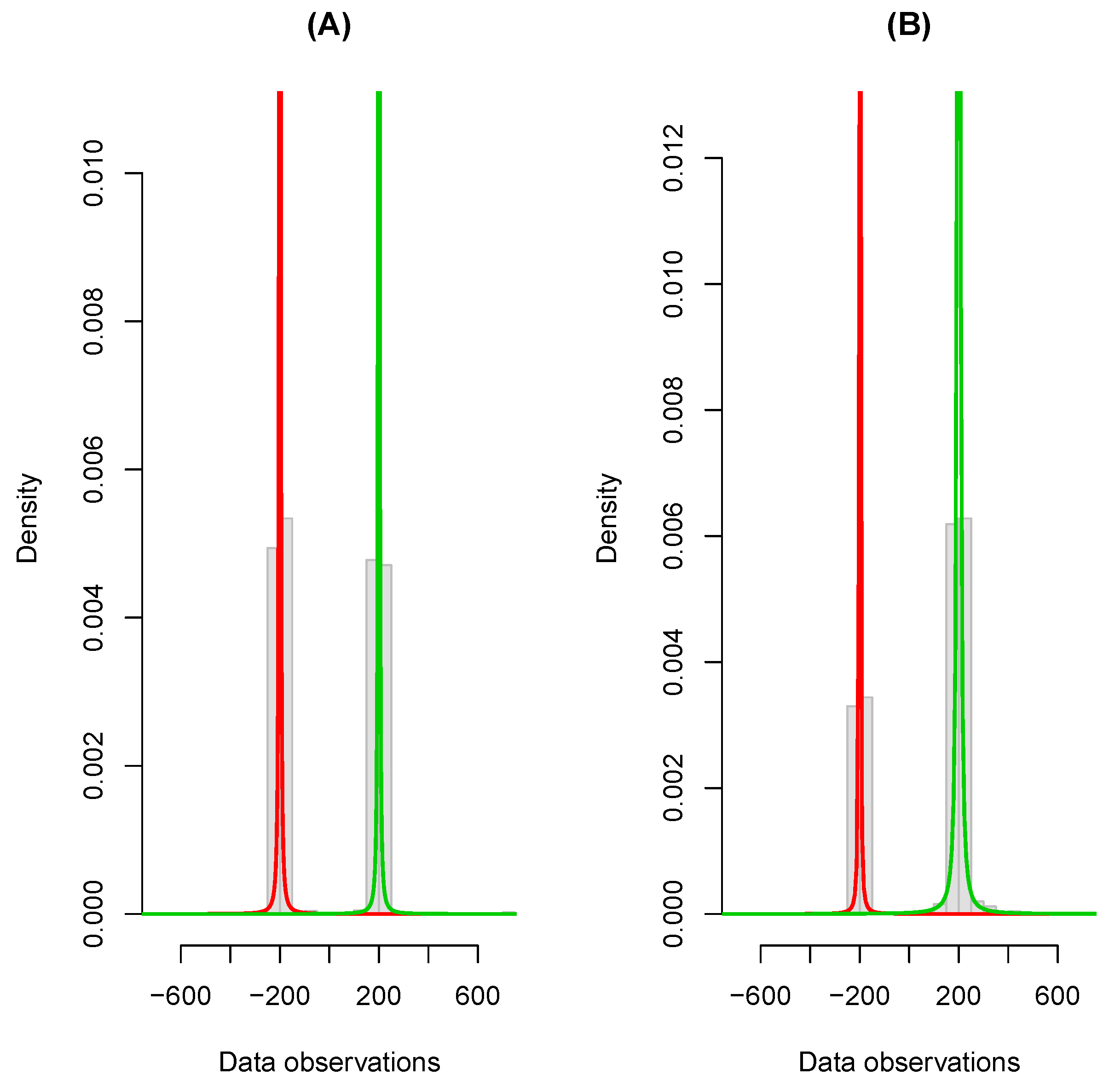
(A)

a two-component Cauchy mixture model with mixing parameters equal to $\underline{p}=(0.5,0.5)$, location parameters $\underline{\alpha }=(-200,200)$ and scale parameters $\underline{\gamma }=(1,1)$;

(B)

a two-component Cauchy mixture model with mixing parameters equal to $\underline{p}=(1/3,2/3)$, location parameters $\underline{\alpha }=(-200,200)$ and scale parameters $\underline{\gamma }=(1,4)$; and

(C)

a four-component Cauchy mixture with $\underline{p}=(0.1,0.3,0.3,0.3)$, $\underline{\alpha }=(-200,200,400,600)$, $\underline{\gamma }=(1,1,1,5)$.

To illustrate the data scenarios, we initially sampled $n=2000$ observations from each dataset. Histograms of the generated data for Scenarios A and B are given in Figure 1, along with the fitted Cauchy mixtures. The corresponding outcome for Scenario C is provided in Figure 2.

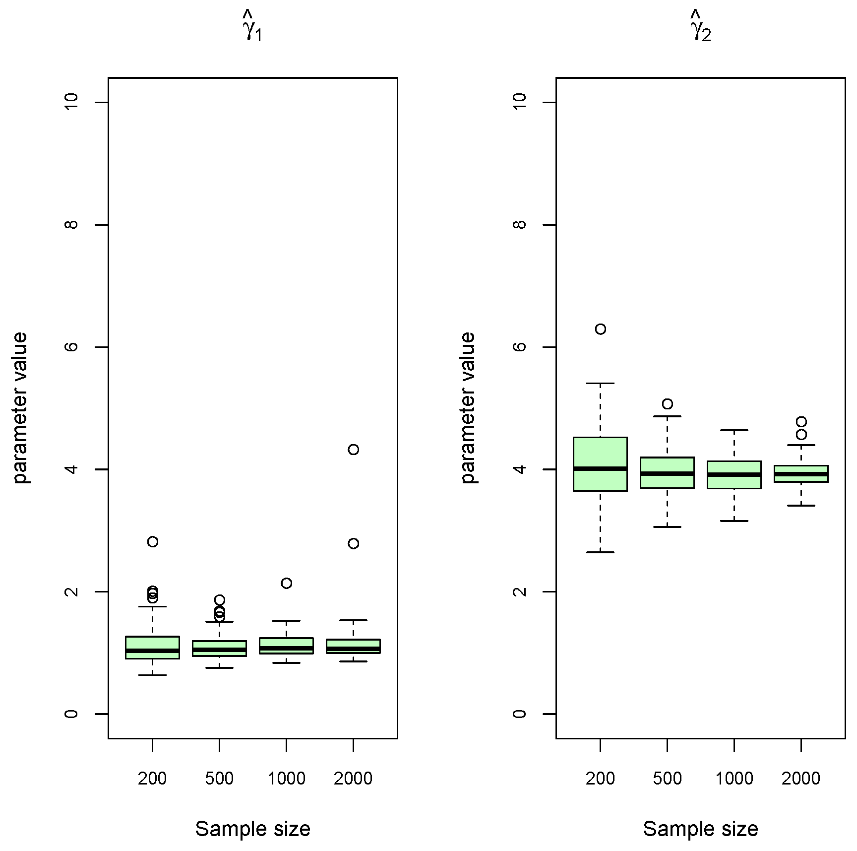
We next carroed out the actual simulation study in order to study the consistency properties of the proposed estimators. For each simulation scenario, we considered sample sizes of $n=200,500,1000$ and 2000; moreover, we replicated the process 200 times for each simulated mixture model. For the initialization of location parameters as described in Section 3, we used Setting (iii) throughout.

For each model parameter, we produced box plots from the 200 estimates and display the results in Figure 3, Figure 4, Figure 5 and Figure 6. We see that the estimates become more accurate and precise as the sample size increases. There is no evidence to suggest that the estimation problem for unequal mixture probabilities and scale parameters (Scenario B) is much harder than for equal probabilities and scale parameters (Scenario A). Consistency also does not appear to be negatively affected when increasing K (Scenario C).

5. Real Data Examples

In this section, the proposed estimation routine for the finite Cauchy mixture model is illustrated and discussed using real data. In identifying the adequate model, we use the Bayesian information criterion ($BIC$) [24], which is a penalized-likelihood criterion. This method identifies the sufficiently complex model considering the model parameters and data sample size,

$$BIC=-2logL\left(\widehat{\Theta }\right)+N_{\theta }logn,$$

(10)

where $N_{\theta }$ is the number of estimated model parameters and n the number of data points used in the fitted model. Then, the smallest value of $BIC$ determines the adequate model in terms of goodness-of-fit/sparsity trade-off. For initializing location parameters, we again use Setting (iii) in all examples, which, to our experience, tends to deliver the best final BIC values.

5.1. Adler Data

This dataset contains 108 observations on a numerical variable, rating, and two categorical variables, instruction and expectation. We are only interested in the rating variable, which are “average ratings of apparent success of people in pictures who were pre-selected for their average appearance of success” [25].

As visualized in Figure 7, the data possess two main clusters, where the right cluster appears skewed to the right, with one extreme and some milder outliers in the right tail. Representing these data by a mixture of Cauchy distributions is then a natural approach.

We firstly fit these models for $K=2$, 3, 4 and 5, using the methods outlined in the previous section, with $S=50$ iterations and consider graphs of $logL$ versus iteration number (Figure 8). We see that, except for $K=2$, all trajectories are monotone. For $K=2$, the maximum likelihood is achieved after only three iterations, with corresponding disparity of $-2logL=910.41$, not improving substantially on the value for $K=1$ (see

Table 2. Adler data: Comparison of $BIC$ of fitted Cauchy mixture model at different K.

	Number of Components (K)
	1	2	3	4	5
$-2logL$	916.56	910.41	867.37	862.76	857.58
$BIC$	925.93	933.83	904.83	914.26	923.13

). It is clear from this figure that $K=5$ yields the largest likelihood overall. To determine the adequate number of components of the mixture, we compute the $BIC$ values for different K, with results summarized in Table 2. One can observe that the smallest value of $BIC$ appears with $K=3$, with the disparity decreasing slightly when increasing K further. The weighted component densities of the fitted 3- and 4-component models are displayed in Figure 9. As a result, we can deduce that the Cauchy mixture model is capable of robustly fitting the data with $K=3$, thereby not requiring a separate component to represent the extreme outlier.

5.2. Melter Data

We consider a chemometric dataset recorded from an industrial glass melter [26]. The system is part of a disposal procedure, where a powder (waste material) is clad in glass. A vessel is continuously filled with powder, while raw glass is discretely introduced in the form of glass frit. Induction coils are positioned around the melter vessel which heat the composition. Resulting from the heating procedure, the mixture becomes molten homogeneously. The melter data consist of 21 variables for which 17,279 samples are available. The recorded variables include fifteen temperature sensors, electric power measurements of four induction coils, the viscosity of the molten glass and the measured electric voltage. We removed the first 700 samples from this dataset, since they involve two plant shutdowns and are therefore misleading for characterizing the operation of the melter process, leaving a reduced set of 16,579 samples.

In this paper, we consider the combined data from five of the temperature sensors, yielding a data vector of length n = 82,895 as an example for the application of the Cauchy mixture model. We initially plot the distribution of the temperature measurements as displayed in Figure 10. The histogram of the data displays bimodality, with many extreme values in the left tail. Obviously, in this case, the mean of the data ($1023.1$) is less than the median (1086) due to the skewness. The interquartile range ($IQR$) of these data is equal to $166.5$.

We fit Cauchy mixture models to this data with $K=1$, 2 and $K=3$. The estimates of model parameters are computed using the EM-type method introduced previously, and the results are summarized in

Table 3. Melter temperature data: Estimated Cauchy mixture parameters for the temperature sensor data.

K	${\widehat{\mathit{p}}}_1$	${\widehat{\mathit{p}}}_2$	${\widehat{\mathit{p}}}_3$	${\widehat{\mathit{\alpha }}}_1$	${\widehat{\mathit{\alpha }}}_2$	${\widehat{\mathit{\alpha }}}_3$	${\widehat{\mathit{\gamma }}}_1$	${\widehat{\mathit{\gamma }}}_2$	${\widehat{\mathit{\gamma }}}_3$
1	1			1086.0			83.2
2	0.198	0.802		878.1	1105.0		27.5	33.0
3	0.225	0.203	0.572	877.5	1055.0	1119.0	31.2	14.1	18.2

. They show that, for $K=2$ and $K=3$, the component with the largest $\widehat{p}$ is associated with $\widehat{\alpha }$ values which are close to the median, but the values of the scale parameters of the individual components decrease quickly to considerably smaller values than $0.5\times IQR$ of the original data.

Figure 11a,c,e displays the plots of the density curves ${\widehat{p}}_j{f}_j\left(x\right|{\widehat{\alpha }}_j,{\widehat{\gamma }}_j)$ of the corresponding mixture model. The right hand side gives, for comparison, the corresponding Gaussian mixture fits. One can see from this the fundamental difference in which Cauchy and Gaussian mixtures operate: The Cauchy mixtures are always centered where relevant peaks of the data are, while some of the Gaussian components try to accommodate the outliers through an extremely flat component. The Cauchy mixtures do not need such a flat component, since their heavy tails can deal with the extreme values already. As a consequence, Cauchy mixtures will generally need fewer components than Gaussian mixtures. In addition, we see in

Table 4. Melter temperature data: Comparison of model disparity ($-2logL$) and $BIC$ between Cauchy mixture and Gaussian mixture fits. For the Cauchy fits with $K=2$ and 3, the minimum disparity was achieved after four and seven iterations, respectively.

K	Cauchy Mixture Model		Gaussian Mixture Model
	$-2log\mathit{L}$	$\mathit{B}\mathit{I}\mathit{C}$	$-2log\mathit{L}$	$\mathit{B}\mathit{I}\mathit{C}$
1	1,044,617	1,044,640	1,095,249	1,095,272
2	988,145	988,202	994,756	994,812
3	970,329	970,419	961,530	961,620

that, while Cauchy mixtures are superior to Gaussian mixture models for $K=1$ and $K=2$, the Gaussian mixture model becomes superior for $K=3$, in terms of both log-likelihood and BIC. It is evident from the provided graphs that densities with $K\ge 4$ certainly do not need to be considered, and that the Cauchy mixture with $K=2$ appears to give visually the best fit.

5.3. Analysis of Image Greyscales

This example considers the analysis of a greyscale image of a symmetrically tiled mosaic. In Figure 12 (left), we illustrate an image which, at first glance, seems to consist mainly of three grey tones. After reading the image into the programming language R and extracting the greyscale information with appropriate tools [27,28], the distribution of greyscales over the 225 × 225 = 50,625 pixels of the image can be displayed in form of a histogram, as in Figure 12 (right). We see that, despite our original impression that there are only three shades of grey present in the mosaic, it is in fact not so clear cut: while there appear to be three major clusters, all of them come with some spread, which is very small for the first two clusters (corresponding to the darker shades), but a bit larger for the third cluster, corresponding to the whitish scales. In fact, one could argue that this last cluster consists of two or more sub-clusters. Furthermore, it appears that there are pixels of outlying grey shade all along the scale; even in the center region where the grey scale is about 0.6 they do not entirely disappear.

It is a relevant task in computer vision to identify the main underlying grey or color shades of a given image [29]. Using the Cauchy mixtures, we are now in an ideal position to do so: there are several sharp peaks but also a large number of outliers.

Motivated by the considerations above, we proceed with fitting the Cauchy mixture model with $K=3$ and $K=4$ components. We see in Figure 13 that in all cases the peaks are clearly identified, with in the latter case, the “white’ cluster being split into a sharper peak, which captures the actual shading of this class, plus a wider one, which captures contaminations or impurities of the original white color. The robustness to outliers of these fitted components is evident from the fitted mixtures. Summarizing, the Cauchy mixture model has done a useful job at identifying the original “true” grey shades of the mosaic.

6. Discussion and Conclusions

The Cauchy mixture provides a suitable model to fit heterogeneous data with outliers. The estimates of model parameters are successfully obtained using an EM-type algorithm, which cycles between the computation of component membership weights using Bayes’ theorem, and the update of component parameters using appropriately weighted quantiles.

Through experimental results, we have shown that the proposed methodology provides sensible model fits, with the estimated location parameters always centered at the data peaks, and which are robust to the presence of the extreme values. We also observed that Cauchy mixtures tend to need less components than Gaussian mixtures in order to achieve a comparable goodness-of-fit.

The properties of the algorithm deserve further discussion. As mentioned above, our M-step does not maximize the expected complete log-likelihood, and there is no mathematical guarantee that it moves the estimated parameters into the direction of its gradient. Indeed, we did observe at some occasions (especially for $K=2$) that both the expected complete likelihood, as well as the incomplete data likelihood slightly decrease for a few iterations (that is, the disparities increase), before returning into the direction of the original trend, and eventually always settling into convergence. While the temporary decrease of the expected complete log-likelihood is not a concern (this can happen in every EM algorithm), the decrease of the likelihood itself is more of an issue, as it lays bare the fact that our methodology is not strictly an EM algorithm [30]. EM algorithms with this rather undesired property have sometimes been referred to as “pseudo-EM” in the literature; we prefer the simpler term “EM-type”. Despite not being strictly an EM algorithm, the methodology has demonstrated to behave convincingly in application and simulation, with excellent robustness properties. From this perspective, one may speculate that a certain resistance of the methodology to “always following the gradient of the likelihood” may in fact be desirable, and it is in this spirit that our method behaves. Further theoretical analysis of these issues appears desirable for future work.

References

1. Aitkin, M.; Francis, B.; Hinde, J.; Darnell, R. Statistical Modelling in R. Oxford Statistical Science Series 35; Oxford University Press: Oxford, UK, 2009. [Google Scholar]
2. Longford, N.T.; D’Urso, P. Mixture models with an improper component. J. Appl. Stat. 2011, 38, 2511–2521. [Google Scholar] [CrossRef]
3. Peel, D.; McLachlan, G.J. Robust mixture modelling using the t distribution. Stat. Comput. 2000, 10, 339–348. [Google Scholar] [CrossRef]
4. Barnett, V. The Study of Outliers: Purpose and Model. J. R. Stat. Soc. Ser. C (Appl. Stat.) 1978, 27, 242–250. [Google Scholar] [CrossRef]
5. Lahmiri, S.; Boukadoum, M. An Ensemble System Based on Hybrid EGARCH-ANN with Different Distributional Assumptions to Predict S&P 500 Intraday Volatility. Fluct. Noise Lett. 2015, 14, 1550001. [Google Scholar]
6. Hua, J.; Huang, M.; Huang, C. Centrality Metrics’ Performance Comparisons on Stock Market Datasets. Symmetry 2019, 11, 916. [Google Scholar] [CrossRef]
7. Raza, N.; Shahzad, S.J.H.; Tiwari, A.K.; Shahbaz, M. Asymmetric impact of gold, oil prices and their volatilities on stock prices of emerging markets. Resour. Policy 2016, 49, 290–301. [Google Scholar] [CrossRef]
8. Reeds, J.A. Asymptotic Number of Roots of Cauchy Location Likelihood Equations. Ann. Stat. 1985, 13, 775–784. [Google Scholar] [CrossRef]
9. Boes, D.C. On the Estimation of Mixing Distributions. Ann. Math. Stat. 1966, 37, 177–188. [Google Scholar] [CrossRef]
10. McLachlan, G.J.; Peel, D. Finite Mixture Models; John Wiley & Sons: New York, NY, USA, 2000. [Google Scholar]
11. Zhang, L.; Gove, J.H.; Liu, C.; Leak, W. A finite mixture of two Weibull distributions for modeling the diameter distributions of rotated-sigmoid, uneven-aged stands. Can. J. For. Res. 2001, 31, 1654–1659. [Google Scholar] [CrossRef]
12. Zaman, M.R.; Roy, M.K.; Akhter, N. Chi-square Mixture of Gamma Distribution. J. Appl. Sci. 2005, 5, 1632–1635. [Google Scholar]
13. Suksaengrakcharoen, S.; Bodhisuwan, W. A new Family of Generalized Gamma Distribution and its Application. J. Math. Stat. 2014, 10, 211–220. [Google Scholar] [CrossRef]
14. Karim, R.; Hossain, P.; Begum, S.; Hossain, F. Rayleigh Mixture Distribution. J. Appl. Math. 2011, 2011, 238290. [Google Scholar] [CrossRef]
15. Sindhu, T.N.; Feroze, N. Bayesian Inference of Mixture of two Rayleigh Distributions: A New Look. J. Math. 2006, 48, 49–64. [Google Scholar]
16. Arnold, B.C.; Beaver, R.J. The skew-Cauchy distribution. Stat. Probab. Lett. 2000, 49, 285–290. [Google Scholar] [CrossRef]
17. Nadarajah, S. Making the Cauchy work. Braz. J. Probab. Stat. 2011, 25, 99–120. [Google Scholar] [CrossRef]
18. Koenker, R.; Bassett, G. Regression Quantiles. Econometrica 1978, 46, 33–50. [Google Scholar] [CrossRef]
19. Bloch, D. A note on the estimation of the location parameter of the Cauchy distribution. J. Am. Stat. Assoc. 1966, 61, 852–855. [Google Scholar] [CrossRef]
20. Rothenberg, T.J.; Fisher, F.M.; Tilanus, C.B. A note on estimation from a Cauchy sample. J. Am. Stat. Assoc. 1964, 59, 460–463. [Google Scholar] [CrossRef]
21. Tiku, M.L.; Suresh, R.P. A new method of estimation for location and scale parameters. J. Stat. Plan. Inference 1992, 30, 281–292. [Google Scholar] [CrossRef]
22. Fried, R.; Einbeck, J.; Gather, U. Weighted Repeated Median Smoothing and Filtering. J. Am. Stat. Assoc. 2007, 102, 1300–1308. [Google Scholar] [CrossRef] [Green Version]
23. Seidel, W.; Mosler, K.; Alker, M. A cautionary note on likelihood ratio tests in mixture models. Ann. Inst. Statist. Meth. 2000, 52, 481–487. [Google Scholar] [CrossRef]
24. Schwarz, G. Estimating the dimension of a model. Ann. Stat. 1978, 6, 461–464. [Google Scholar] [CrossRef]
25. Fox, J.; Weisberg, S.; Price, B. carData: Companion to Applied Regression Data Sets, R Package Version 3.0-2; 2018. Available online: https://CRAN.R-project.org/package=carData (accessed on 20 March 2019).
26. Liu, X.; Xie, L.; Kruger, U.; Littler, T.; Wang, S.-Q. Statistical-based monitoring of multivariate non-gaussian systems. AIChE J. 2008, 54, 2379–2391. [Google Scholar] [CrossRef]
27. Mouselimis, L. OpenImageR: An Image Processing Toolkit, R Package Version 1.1.4.; 2019. Available online: https://CRAN.R-project.org/package=OpenImageR (accessed on 30 January 2019).
28. Beleites, C. Arrayhelpers: Convenience Functions for Arrays, R Package Version 1.0-20160527; 2016. Available online: https://CRAN.R-project.org/package=arrayhelpers (accessed on 30 January 2019).
29. Nguyen, T.M.; Wu, Q.M.J.; Mukherjee, D.; Zhang, H. A Bayesian Bounded Asymmetric Mixture Model with Segmentation Application. IEEE J. Biomed. Health Inform. 2014, 18, 109–119. [Google Scholar] [CrossRef] [PubMed]
30. Dempster, A.P.; Laird, N.M.; Rubin, D.B. Maximum Likelihood from Incomplete Data via the EM Algorithm. J. R. Stat. Soc. Ser. B 1977, 39, 1–38. [Google Scholar] [CrossRef]
Figure 1. Simulated data: Scenario A (left); and Scenario B (right). The plotted curves correspond to the fitted component densities weighted by the estimated components probabilities at K = 2 . Note that the densities are truncated at the top.
Symmetry 11 01186 g001
Figure 2. Simulated data, Scenario C: The plotted curves correspond to the fitted component densities weighted by the estimated components probabilities.
Symmetry 11 01186 g002
Figure 3. Simulated data, Scenario A: Box plots of estimated Cauchy mixture parameters at different sample sizes of n = 200 , 500 , 1000 , and 2000 (when p 1 = p 2 = 0.5 , α 1 = 200 , α 2 = 200 , γ 1 = γ 2 = 1 ).
Symmetry 11 01186 g003aSymmetry 11 01186 g003b
Figure 4. Simulated data, Scenario B: Box plots of estimated Cauchy mixture parameters at different sample sizes of n = 200 , 500 , 1000 , and 2000 (when p 1 = 1 / 3 , p 2 = 2 / 3 , α 1 = 200 , α 2 = 200 , γ 1 = 1 and γ 2 = 4 ).
Symmetry 11 01186 g004aSymmetry 11 01186 g004b
Figure 5. Simulated data, Scenario C: Box plots of estimated Cauchy mixture mixing parameters at different sample sizes of n = 200 , 500 , 1000 , and 2000 (when p ̲ = ( 0.1 , 0.3 , 0.3 , 0.3 ) , α ̲ = ( 200 , 200 , 400 , 600 ) and γ ̲ = ( 1 , 1 , 1 , 5 ) ) .
Symmetry 11 01186 g005
Figure 6. Simulated data, Scenario C: Box plots of estimated Cauchy mixture location and scale parameters at different sample sizes of n = 200 , 500 , 1000 , and 2000 (when p ̲ = ( 0.1 , 0.3 , 0.3 , 0.3 ) , α ̲ = ( 200 , 200 , 400 , 600 ) and γ ̲ = ( 1 , 1 , 1 , 5 ) ) .
Symmetry 11 01186 g006
Figure 7. Adler data: Histogram of average rating distribution.
Symmetry 11 01186 g007
Figure 8. Log-likelihood trajectories for Adler data, with S = 50 iterations.
Symmetry 11 01186 g008
Figure 9. Fitted Cauchy mixtures for average ratings from Adler data: (Left) K = 3 ; and (right) K = 4 .
Symmetry 11 01186 g009
Figure 10. Melter data: Histogram of 82,895 temperature measurements.
Symmetry 11 01186 g010
Figure 11. Fitted Cauchy (left); and Gaussian (right) mixtures to melter temperature data. The displayed curves correspond to the fitted component densities weighted by the estimated component probabilities.
Symmetry 11 01186 g011
Figure 12. (Left) Image of tiled mosaic; and (right) histogram of grey scale distribution of image (1 = white, 0 = black).
Symmetry 11 01186 g012
Figure 13. Fitted Cauchy mixtures for grey scales from the tiled mosaic: (Left) K = 3 ; and (right) K = 4 .
Symmetry 11 01186 g013