Article

Symmetry Analysis of an Interest Rate Derivatives PDE Model in Financial Mathematics

by
Bosiu C. Kaibe
* and
John G. O’Hara
Centre for Computational Finance and Economic Agents, University of Essex, Colchester CO4 3SQ, UK
*
Author to whom correspondence should be addressed.
Symmetry 2019, 11(8), 1056; https://doi.org/10.3390/sym11081056
Submission received: 23 July 2019 / Revised: 8 August 2019 / Accepted: 12 August 2019 / Published: 16 August 2019

Abstract

:
We perform Lie symmetry analysis to a zero-coupon bond pricing equation whose price evolution is described in terms of a partial differential equation (PDE). As a result, using the computer software package SYM, run in conjunction with Mathematica, a new family of Lie symmetry group and generators of the aforementioned pricing equation are derived. We furthermore compute the exact invariant solutions which constitute the pricing models for the bond by making use of the derived infinitesimal generators and the associated similarity reduction equations. Using known solutions, we again compute more solutions via group point transformations.

1. Introduction

In order to raise capital, firms and governments normally do so by issuing financial instruments known as bonds. A bond is a financial contract under which the issuer promises to pay a counter-party intervals of payments (coupons) and a lump sum of money (termed principal) at the end of the agreed time. The coupon payments are usually periodical. If there are no payments made in the interim but only one payment of a lump sum of money at the agreed time, then this type of bond is called a zero-coupon bond, and the lump sum paid is called the face value of the bond. Valuation of the bond over a specific term depends crucially on the random fluctuations of the interest rate market. If the life span of the contract is short, interest rates are normally assumed to be deterministic or constant, but, with a long life span, it will be unrealistic to assume them to be still deterministic. This then led to other ways being explored to address this issue, and several stochastic interest rate models were developed in the past years. The most commonly used are the Vasicek model [1] and the Cox–Ingersoll–Ross (CIR) model [2] as both have proved to be tractable and empirically relevant in capturing properties of interest rates. It has been shown in Wilmott et al. [3] that, with the spot rate following a stochastic differential equation
d r = a ( r , t ) d t + b ( r , t ) d X ,
where X is a Wiener process, the value of a zero-coupon bond W ( r , t ; T ) , with expiry at t = T , can be obtained from solving the partial differential equation (PDE)
W t + b 2 2 W r r + ( a κ b ) W r r W = 0 ,
subject to W ( r , T ) = 1 . Pricing of financial securities has been one of the major concerns to financial markets practitioners as discrepancies in financial products prices can lead to great profits to market participants. This then led to special attention being given to the development of financial products such as derivatives. One of the pioneering breakthroughs in the pricing of financial products was the research work by Black and Scholes [4]. The main subject of their work was a linear parabolic differential equation:
u t + 1 2 S 2 σ 2 u S S + r ( S u S u ) = 0 ,
which upon solving produced interesting results that were then used as the pricing models for contingent claims call and put options. The Black–Scholes Merton model, which it was later called due to the contribution made by Merton [5], have been used as the main vehicle for pricing many financial products whose price dynamics were expressed in terms of partial differential equations. After this discovery, Black–Scholes valuation framework was extended to price many other financial products, among them: bond options and other interest rate derivatives. In the case of bond options, a challenge met was the issue of taking into account the convergence of a bond price to par at maturity. Due to this, it is important that correct modelling of stochastic behaviours of interest rates, especially the term structure of the interest rate through time, are carefully implemented when constructing realistic and reliable valuation models of interest rate derivatives. Analytic approaches and numerical methods have been mostly favoured in solving differential equations even though analytic approaches seem to be more preferred as they provide much information on the pricing models. This fact is supported by an increasing number of research papers published in recent years using this approach. Among analytical approaches, we focus our attention on Lie symmetry analysis that have played a vital role in solving PDE models arising in the field of mathematical finance. We recognise among others the work by Ibragimov and Gazizov [6], who introduced the idea of Lie symmetry analysis in finance problems when analysing the Black–Scholes pricing equation. Goard [7] also contributed by proposing new and simple solutions to the bond pricing Equation (2) via symmetry analysis. Pooe et al. [8], using transformations to reduce the bond-pricing equation to a heat equation, obtained the solution to the zero-coupon bond via usage of those transformations. Sinkala and colleagues in [9] computed new prices for the bond PDE model with special consideration given to Vasicek and CIR models. In recent years, Khalique et al. [10] have proposed new invariant solutions and conservation laws for the Vasicek pricing equation model. Lie symmetry analysis, as originated in studies by mathematician Sophus Lie, has proved in studies to be one of the prominent tools for obtaining analytical solutions for differential equations.
Most interest rate models do not satisfy the following important two properties: mean-reversion and positivity of interest rate. A well known interest rate model that does not satisfy the second property is the Vasicek interest rate model as its interest rate can be negative. Luo et al. [11], using the combination of the Ornstein–Unlenbeck process (satisfying mean-reversion property) and Bessel process (satisfying positivity property), derived and proposed the following functional interest rate model:
d X t = η ( t ) X t + ϵ ( t ) X t d t + σ ( t ) d Z t ,
where Z t t 0 is a Brownian motion, and ϵ , η , σ are given functions of t. In this setup, r t = f ( X t , t ) is modelled as a function of Markov state variable X t and time t. If f’s range is confined to only positive real values, then this enables avoidance of negative interest rates, which are usually occurring in Vasicek models. This interest rate model embeds most known interest rate models that can be deduced for different choices of f, η , ϵ and σ . Using this functional interest rate model, it can be shown that, for an interest rate derivative such as a zero-coupon bond, its price dynamics are described in terms of the following partial differential equation
v t ( x , t ) + σ 2 2 v x x ( x , t ) + η x + ϵ x v x ( x , t ) r v ( x , t ) = 0 .
Numerical methods such as binomial trees, Monte Carlo simulation, and finite-difference methods are normally tools used to value financial products such as interest rate derivatives. In this work, we use an analytical approach of Lie symmetry analysis to derive four Lie point symmetries plus an additional infinite sub-algebra, and we make use of these symmetries to deduce three types of closed-form solutions for this interest rate derivative pricing equation associated with the functional interest rate model. We further analyse the obtained solutions by investigating their application to the Vasicek interest rate model numerically.
The paper is put together as follows: in Section 2, we derive the PDE model associated with this zero-coupon bond model and perform Lie symmetry analysis to the zero-coupon bond pricing Equation (5). In Section 3, we deduce exact invariant solutions of the model from the associated infinitesimal generators. In Section 4, we obtain numerical solutions, applications made to the Vasicek model, and analyse our findings thereafter. Concluding remarks of the paper are given in Section 5.

2. Governing Equation and Symmetry Analysis

Consider a bond that does not pay any coupons but pays h ( r T ) at expiry time T. Using the functional interest rate model in Equation (4), the payoff of this zero-coupon bond is expressed as h ( f ( X T , t ) ) and its price given by v ( X t , t ) , where
v ( x , t ) = E e t T f ( X s , s ) d s h ( f ( X T , T ) ) | X t = x , t < T .
Applying the Feynman–Kac formula on Equation (6), this results in v ( x , t ) satisfying the partial differential equation in Equation (5).
Computation of Lie symmetries is an algorithmic process in nature, but there are nowadays many computational packages available to assist in the calculations. In this work, we have used computer package SYM [12] together with Mathematica (11.0, Wolfram S., New York, USA) for our computations. From Lie’s symmetry theory, the construction of the symmetry group is equivalent to the determination of the infinitesimal generator
λ = ξ ( x , t , u ) x + τ ( x , t , u ) t + ϕ ( x , t , u ) u ,
with infinitesimals ξ , τ and ϕ functions of variables ( x , t , u ) . These infinitesimals are obtained from solving Lie’s invariance condition. That is, if p r ( 2 ) λ is the second extension or prolongation of λ given by
p r ( 2 ) λ = λ + ϕ x u x + ϕ t u t + ϕ x x u x x + ϕ x t u x t + ϕ t t u t t ,
where
ϕ t = D t ( ϕ ξ u x τ u t ) + ξ u x t + τ u t t , ϕ x = D x ( ϕ ξ u x τ u t ) + ξ u x x + τ u x t , ϕ x x = D x 2 ( ϕ ξ u x τ u t ) + ξ u x x x + τ u x x t ,
and “D” represents the total derivative, i.e.,
D x R = x R + u x u R + u x x u x R + u x t u t R + ,
then, the invariance condition constituted by our model (call it F) is p r ( 2 ) λ F | F = 0 = 0 [6] or
p r [ 2 ] λ u t ( x , t ) + σ 2 2 u x x ( x , t ) + η x + ϵ x u x ( x , t ) r u ( x , t ) | ( 5 ) = 0 .
Using SYM to solve Equation (9), β = σ 2 2 , the infinitesimals are computed as
τ = e 2 η t c 1 η e 2 η t c 2 η + c 3 ξ = x e 2 η t c 1 + x e 2 η t c 2 ϕ = 1 ϵ β + r η + x 2 η β e 2 η t u c 1 r η e 2 η t u c 2 + u c 4 + B ( x , t ) ,
where c 1 , c 2 , c 3 , c 4 are any constants and B ( x , t ) is a solution of Equation (5). The arbitrary constants in Equation (10) constitute an infinite dimensional Lie algebra of symmetries and they are given as
λ 1 = t , λ 2 = e 2 η t η t + x e 2 η t x r e 2 η t η u u , λ 3 = e 2 η t η t + x e 2 η t x + 1 ϵ β + r η + x 2 η β u e 2 η t u , λ 4 = u u , and λ B = B ( x , t ) u .
Using the Lie point symmetries in Equation (11), we obtain the point transformations or one-parameter groups of symmetries ψ : ( x , t , u ) ( x ˜ , t ˜ , u ˜ ) of the model in Equation (5) with u ˜ ( x ˜ , t ˜ ) as its solution. Making use of the five generators in Equation (11) and solving the following ordinary differential equations:
d x ˜ d κ = ξ ( x ˜ , t ˜ , u ˜ ) , d t ˜ d κ = τ ( x ˜ , t ˜ , u ˜ ) , d u ˜ d κ = ϕ ( x ˜ , t ˜ , u ˜ ) ,
taking into consideration the initial conditions
x ˜ | κ = 0 = x , t ˜ | κ = 0 = t , u ˜ | κ = 0 = u ,
we obtain the following corresponding five one-parameter groups of symmetry for Equation (5)
ψ 1 : ( x , t , u ) ( x , t + κ 1 , u ) ψ 2 : ( x , t , u ) x e ( e 2 η t κ 2 ) , 1 2 η ln 2 η κ 2 η e 2 η t 2 η , e r κ 2 η e 2 η t u ψ 3 : ( x , t , u ) x e e 2 η t κ 3 , 1 2 η ln 2 η κ 3 η e 2 η t 2 η , u e 1 + ϵ β r η x 2 η β e 2 η t κ 3 ψ 4 : ( x , t , u ) ( x , t , u e κ 4 ) ψ 5 : ( x , t , u ) ( x , t , u + B ( x , t ) e κ 5 ) ,
with κ i , i = 1, 2, …, 5 representing any constant.

3. Exact Invariant Solutions of Equation (5)

In this section, we use infinitesimal generators obtained to deduce similarity variables from associated characteristic equations to get a family of new invariant solutions of the zero-coupon bond model associated with functional interest rate model. Given any partial differential equation of the form
Δ ( x , t , u , u x , u t , u x x , u x t , u t t ) = 0 ,
a function u = θ ( x , t ) resulting from its invariance under the associated infinitesimal generator λ is regarded as its invariant solution provided:
λ ( u θ ( x , t ) ) = 0 when u = θ ( x , t ) .
Making use of this important concept, we deduce the characteristic equations associated with the infinitesimal generators in Equation (11) to obtain the following three types of close-form invariant solutions of Equation (5) as deduced in Examples 1–3 below.
Example 1.
Considering the infinitesimal generator λ 1 and solving the associated characteristic equations
d t 1 = d x 0 = d u 0 ,
this results in the following two invariants J 1 = x , and J 2 = u . The invariant solution is given by J 2 = ω ( J 1 ) , i.e., u = ω ( x ) .
Substituting u = ω ( x ) in Equation (5), this reduces the model to the following ODE:
r x ω ( x ) + ( ϵ x 2 η ) ω ( x ) + β x ω ( x ) = 0 .
Solving this differential equation, we get the following result with the solution
ω ( x ) = c 1 M m , n , η x 2 2 β + c 2 U m , n , η x 2 2 β x ρ ,
where
m = 1 2 ( η + r ) β η ϵ η β , n = 1 2 3 β ϵ β , ρ = β ϵ β
and c 1 , c 2 are any chosen constants. M ( a , b , . ) and U ( a , b , . ) are special types of the Kummer M and U described in more depth in reference [13]. Therefore, the derived explicit exact invariant solutions for the zero-coupon bond Equation (5) associated with λ 1 are
u ( x , t ) = c 1 M m , n , η x 2 2 β + c 2 U m , n , η x 2 2 β x ρ ,
where m, n, ρ are as above.
Example 2.
Considering the infinitesimal generator λ 2 and following the same procedure as in Example 1 above, we solve the characteristic equations to obtain the invariants
ζ = t + ln x η , u ( x , t ) = x r η ω t + ln x η = x r η ω ζ ,
and the similarity function ω = ω ( ζ ) satisfies the following similarity reduction equation:
r ( r β + ( β ϵ ) η ) ω ( ζ ) + ( 2 r β β η + ϵ η ) ω ( ζ ) + β ω ( ζ ) = 0 .
Solving this differential equation, we result with the following solution
ω ( ζ ) = e ζ ( r β + β η ϵ η ) c 1 + e r ζ c 2 .
Therefore, the derived explicit exact invariant solutions of the zero-coupon bond Equation (5) associated with λ 2 are
u ( x , t ) = x r η e ζ ( r β + β η ϵ η ) c 1 + e r ζ c 2 ,
where c 1 , c 2 are arbitrary constants and ζ is as defined in Equation (22).
Example 3.
Considering lastly the infinitesimal generator λ 3 , the invariants are computed from the characteristic equations and are obtained as
ζ = t ln x η , u ( x , t ) = e x 2 η 2 β x 1 ϵ β + r η ω t ln x η ,
and the similarity function ω = ω ( ζ ) satisfies the following similarity reduction equation:
( r 2 η ) ( r β ( β + ϵ ) η ) ω ( ζ ) + ( 2 r β + 3 β η + ϵ η ) ω ( ζ ) + β ω ( ζ ) = 0 .
Solving this differential equation, we receive results with the following solution:
ω ( ζ ) = e ζ ( r β β η ϵ η ) β c 1 + e ζ ( r 2 η ) c 2 .
Hence, the derived explicit exact invariant solutions of the zero-coupon bond Equation (5) associated with λ 3 are
u ( x , t ) = e x 2 η 2 β x 1 ϵ β + r η e ζ ( r β β η ϵ η ) β c 1 + e ζ ( r 2 η ) c 2 ,
where c 1 , c 2 are arbitrary constants and ζ is as defined in Equation (26). This concludes the calculations of invariant solutions as λ 4 does not have any invariants.

3.1. New Solutions via Group Point Transformations

In this section, we make use of known solutions in Equations (25) and (29) to compute new solutions from them using group point transformations in Equation (14). An important concept about Lie’s group theory is its ability to transform solutions of a differential equation into other solutions of the same equation using point transformations. If λ in Equation (7) is the group generator admitted by Equation (5) and u = w ( x , t ) is any of the equation solutions, then u ˜ = w ˜ ( x ˜ , t ˜ ) will also define another solution of Equation (5) obtained via group point transformations. That is, if we replace x ˜ , t ˜ , and u ˜ in transformations in Equation (14) and solve for u, this then results with new solutions for Equation (5). We give an illustrate of this point by making use of ψ 1 in Equation (14). With this transformation, since x ˜ = x and u ˜ = u , both solutions in Equations (25) and (29) are transformed to new solutions, whereby t in both equations is replaced by ( t κ 1 ) . That is, Equations (25) and (29) will only be affected for ζ as it now changes to ( t κ 1 ) + ln x η and ( t κ 1 ) ln x η , respectively, for Equations (25) and (29).

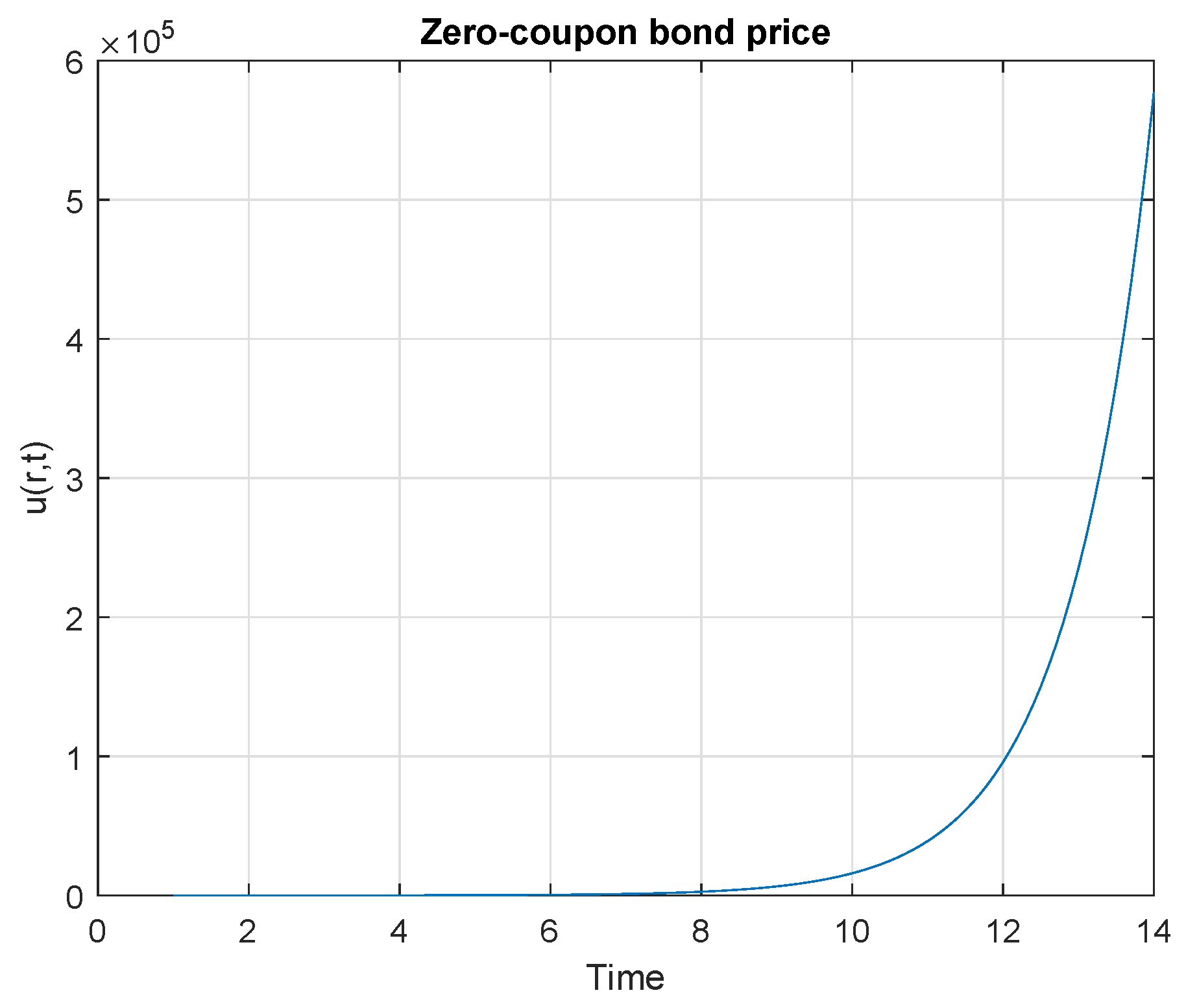
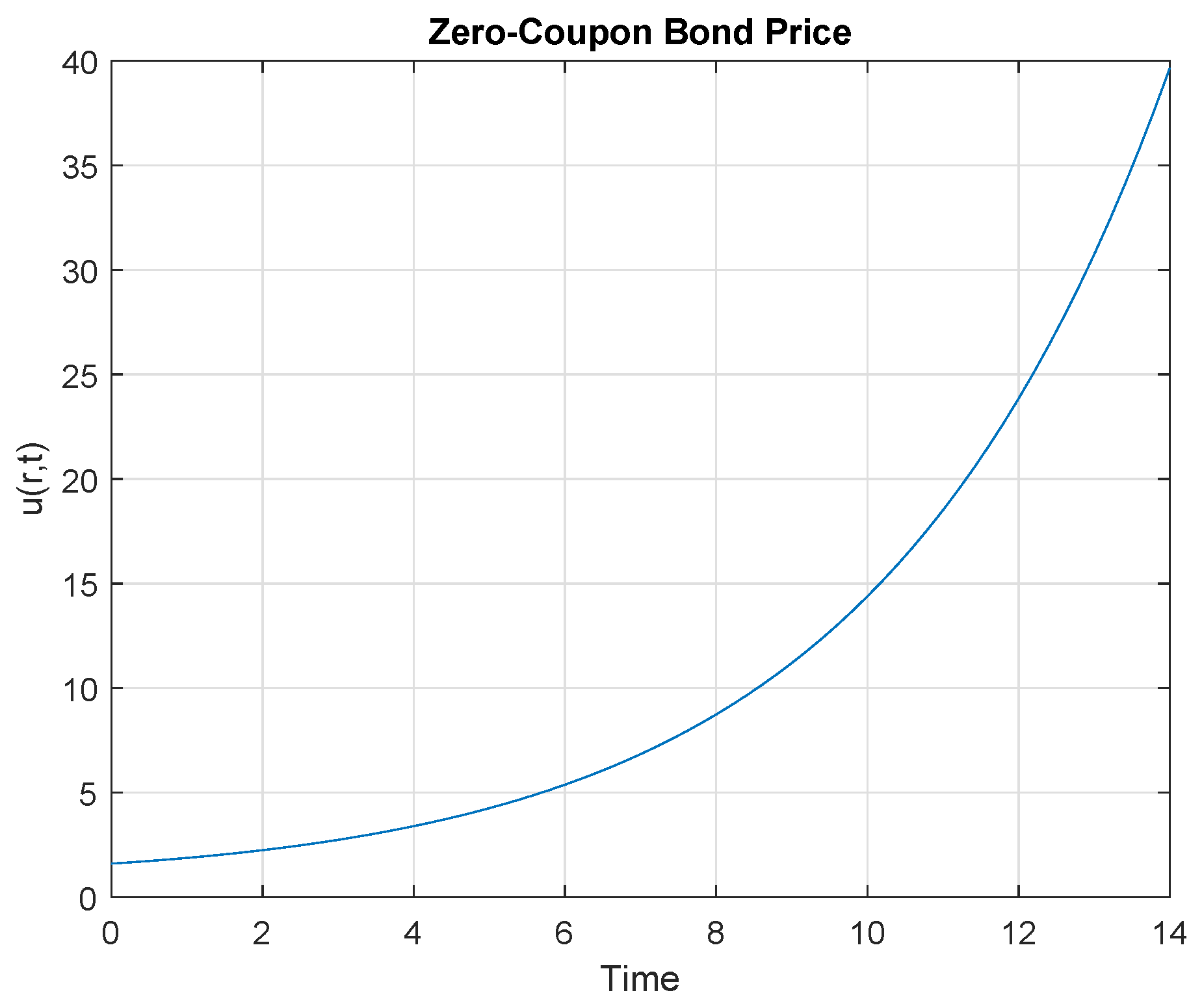
4. Results Discussion

Numerical solutions are deduced in this section to emphasise the novelty of Lie’s group theory. We use the newly obtained explicit solutions in Equations (25) and (29); and application is done to the Vasicek interest rate model. It has been shown in Chern [14] that, with parameters: x = r + α , ϵ = 0 and η = κ , the functional model can be transformed to the Vasicek model. Again, with parameters: β = 2 η , α = ( σ 2 + 2 ϵ ) / ( 8 η ) , r = 1 4 x 2 , a functional model can be transformed into the CIR model, and so on. The parameters chosen for illustration are as follows:
  • interest rate (risk-free) r = 0.90,
  • volatility σ = 0 . 80 ,
  • parameter α = 0 . 01 ,
  • parameter η = 0 . 5 ,
  • constant 1 c 1 = 1 ,
  • constant 2 c 2 = 0 . 5 ,
  • time to expiration T = 14 years.
We illustrate the solutions in Figure 1 and Figure 2 for the newly explicit solutions associated with λ 2 and λ 3 .
A zero-coupon bond being a simple agreement indicating a time a single lump sum of money will be exchanged between counter-party A (bond-seller, say company) and counter-party B (bond-buyer, say investor), an important question that one may ask is what should happen to the prices of a zero-coupon bond as time passes? As Bodie et al. [15] on page 433 illustrates with an example, the zero-coupon bond is expected to sell for par value at maturity, but, before then, it should sell at a discount from par value due to the time value of money. In fact, when the interest rate is constant, a zero-coupon bond price should increase at exactly the rate of interest. We observe that the curves of the explicit exact invariant solutions obtained in Section 3, an analysis made with the Vasicek model, are smooth and monotonically increasing with respect to time towards the maturity of the bond. Section 3.1, using group ψ 1 to illustrate the novelty of the method, graphs in Figure 1 and Figure 2 will still be the same shape under ψ 1 , but they will be horizontally shifted to the right (or translated) by κ i units ( κ i > 0 ). These results show some resemblance to the graphs in Bodie et al. [15], and Goard [7]; and thus emphasise the important point that, as time passes, the price of the zero-coupon bond indeed increases at the rate of interest. Again, we observe that solutions of the zero-coupon bond pricing equation have a direct mapping with one another through point transformations; this then emphasises an important concept of Lie symmetry analysis as mentioned in Section 3.1.

5. Conclusions

In this work, Lie symmetry analysis has been performed on a zero-coupon bond pricing equation in mathematical finance. It has been shown that the zero-coupon bond pricing equation admits four point symmetries plus an additional infinite dimensional sub-algebra λ B , which are the symmetries we propose for this model. Using the obtained infinitesimal generators, exact solutions of the zero-coupon bond model have been computed as invariant solutions. The novelty of the solutions has been resembled as graphs where we observed an exponential growth by prices of the zero-coupon bond equation. There seems to be direct relationship between solutions of bond options under functional interest rate modelling and solutions under usual interest rate models, and we believe direct mappings via Lie symmetry analysis could link them. A good model therefore depends entirely on the choices made from parameters r, ϵ , σ and η .
It is a well known fact that interest rate derivatives are much more complex to value than equity and foreign exchange derivatives due to the behaviour of an interest rate being more complicated as compared to that of stock prices or an exchange rate. Due to this, numerical computations seem to be more appreciated in the valuation of interest rate derivatives as there are not many analytical expressions for interest rate derivatives. The model in Equation (5) can be referred to as a functional PDE model due to interest rate associated with it modelled as a certain functional transformation of the underlying state variable. This functional transformation as we have noted does not only embed the known single factor interest rate models, but also provides a flexible approach and analytical scheme for constructing many more new models to expand the existing family of interest rate financial models. Again, as pointed out in [11], this model can provide great benefits in numerical computations as well.
Using the solutions in Equations (25) and (29), the important concept of Lie symmetry analysis has been verified in Section 3.1, since, through group point transformations, unknown solutions have been derived from known solutions. This then suggests that there exists a mapping that transforms functional interest rate derivative PDE models into models like the Vasicek equation and other model equations; in addition, a mapping of solutions of functional interest derivative PDE models to solutions of known interest rate models’ PDE equations. Therefore, with these facts, we want to believe that this work can contribute to the pricing of interest rate derivatives models and it can expand the minute number of analytical expressions that are currently available for pricing interest rate derivatives. Again, with the range of f ( X t , t ) = r t restricted to positive real values, this then can enable one to avoid negative interest rates, such as those usually occurring in the Vasicek model. The model in Equation (4) combines the Ornstein–Unlenbeck process and the Bessel process; therefore, it satisfies both the two important properties of the interest rate models as mentioned in the Introduction, and it can, as a result, enable one to construct new models with ease due to its flexibility. The CIR models satisfy both properties of the interest rate model, since it is also embedded in this model; through application of functional transformations presented in Section 4, a mapping connecting solutions of the functional PDE model and the CIR equation can be obtained in the same approach the Vasicek model was dealt with. In as much as Chern [14] states that literature regarding this approach is still minute, we would like to believe that this model, due to its functional approach to modelling interest rates and its ability to provide a unified framework for representing existing single factor interest rate models, can play a vital role in finance literature for pricing interest rate derivatives to expand existing analytical expressions for debt securities. This fact is supported by the valuations approach and application of Lie symmetry analysis, used to deduce closed-form invariant solutions for this interest rate derivative model. The Heath–Jarrow–Morton (HJM) Model, which specifies the volatilities of all instantaneous forward rates, only has inputs that are the underlying and a measure of its volatility. We notice from the model in Equation (4) that the underlying is resembled by a Markov state variable X t and uncertainty associated with the model resembled by σ ( t ) , which are both incorporated in the model. Therefore, like other known models, a mapping connecting HJM models and functional models should exist, and it is part of this work that we plan to explore further in future work.

Author Contributions

Conceptualization, B.C.K. and J.G.O.; Formal Analysis, Methodology, Writing-Original draft, software, validation, visualization, Writing-review and Editing, B.C.K.; Supervision, J.G.O.

Funding

This research received no external funding.

Acknowledgments

B.C.K. is a Commonwealth Scholar, funded by the UK government; and he would like to thank the Commonwealth Scholarship Commission (CSC) for financial support.

Conflicts of Interest

The authors declare no conflict of interest.

References

  1. Vasicek, O. An equilibrium characterization of the term structure. J. Financ. Econ. 1973, 5, 177–188. [Google Scholar] [CrossRef]
  2. Cox, J.C.; Ingersoll, J.E.; Ross, S.A. An intertemporal general equilibrium model of asset prices. Econometrica 1985, 53, 363–384. [Google Scholar] [CrossRef]
  3. Wilmott, P.; Dewynne, J.; Howison, S. Option Pricing: Mathematical Models and Computation; Oxford Financial Press: Oxford, UK, 1994. [Google Scholar]
  4. Black, F.; Scholes, M. The Pricing of Options and Corporate Liabilities. J. Political Econ. 1973, 81, 637–654. [Google Scholar] [CrossRef] [Green Version]
  5. Merton, R.C. Theory of rational option pricing. Bel. J. Econ. Man. Sci. 1973, 4, 141–183. [Google Scholar] [CrossRef]
  6. Gazizov, R.K.; Ibragimov, N.H. Lie symmetry analysis of differential equations in finance. Nonlinear Dyn. 1998, 17, 387–407. [Google Scholar] [CrossRef]
  7. Goard, J. New solutions to the bond-pricing equation via Lie’s classical method. Math. Comput. Model. 2000, 32, 299–313. [Google Scholar] [CrossRef]
  8. Pooe, C.A.; Mohomed, F.M.; Soh, C.W. Fundamental solutions for zero-coupon bond pricing models. Nonlinear Dyn. 2004, 36, 69–76. [Google Scholar] [CrossRef]
  9. Sinkala, W.; Leach, P.G.L.; O’ Hara, J.G. Zero-coupon bond prices in the Vasicek and CIR models: Their computation as group-invariant solutions. Math. Methods Appl. Sci. 2008, 31, 665–678. [Google Scholar] [CrossRef]
  10. Khalique, C.M.; Motsepa, T. Lie symmetries, group-invariant solutions and conservation laws of the Vasicek pricing equation of mathematical finance. Phys. A Stat. Mech. Appl. 2018, 505, 871–879. [Google Scholar] [CrossRef]
  11. Luo, S.; Yan, J.; Zhang, Q. A functional transformation approach to interest rate modelling. In Stochastic Processes, Finance and Control: A Festschrift in Honor of Robert J Elliott; World Scientific: Hackensack, NJ, USA, 2012; pp. 303–315. [Google Scholar]
  12. Dimas, S.; Soubelis, D.T. SYM: A new symmetry—Finding package for Mathematica. In Proceedings of the 10th International Conference in Modern Group Analysis, Larnaca, Cyprus, 24–31 October 2004; Ibragimov, N.H., Sophocleous, C., Damianou, P.A., Eds.; University of Cyprus Press: Nicosia, Cyprus, 2005; pp. 64–70. [Google Scholar]
  13. Abramowitz, M.; Stegun, I.A. Handbook of Mathematical Functions; Dover Publication, INC: New York, NY, USA, 1972. [Google Scholar]
  14. Chern, I.L.; Financial Mathematics. Department of Mathematics, National Taiwan University and University of Hong Kong. Available online: http://www.math.ntu.edu.tw/~chern/notes/finance.pdf (accessed on 14 December 2017).
  15. Bodie, Z.; Kane, A.; Marcus, A. Investments, 5th ed.; McGraw-Hill Education: New York, NY, USA, 2003. [Google Scholar]
Figure 1. Explicit exact invariant solutions associated with λ 2 .
Symmetry 11 01056 g001
Figure 2. Explicit exact invariant solutions associated with λ 3 .
Symmetry 11 01056 g002

