A Path-Planning Performance Comparison of RRT*-AB with MEA* in a 2-Dimensional Environment


Abstract
:1. Introduction
2. Related Work
3. Methodology
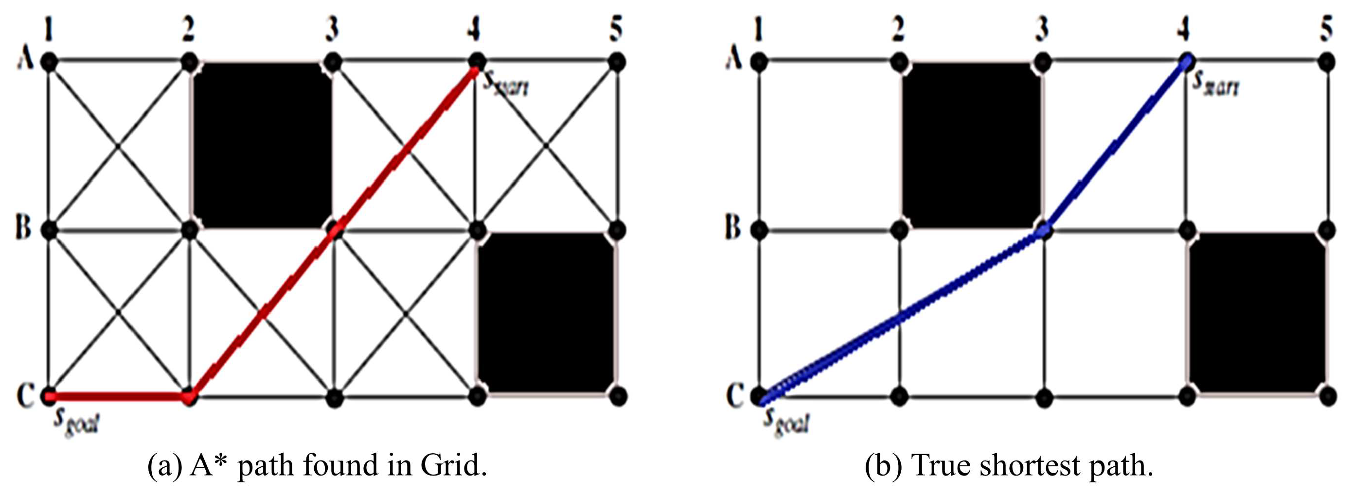
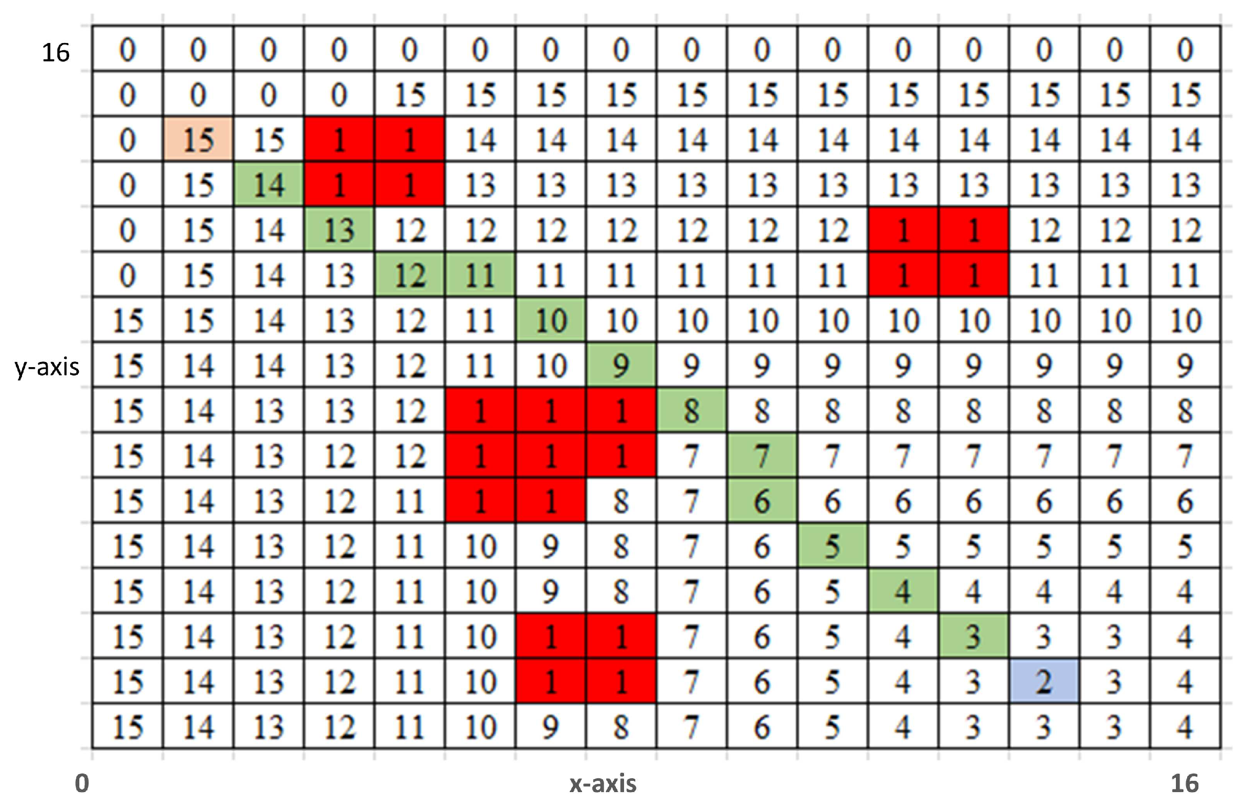
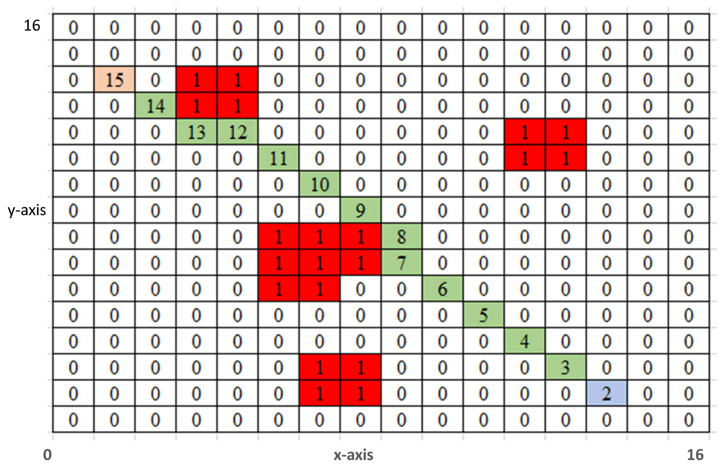
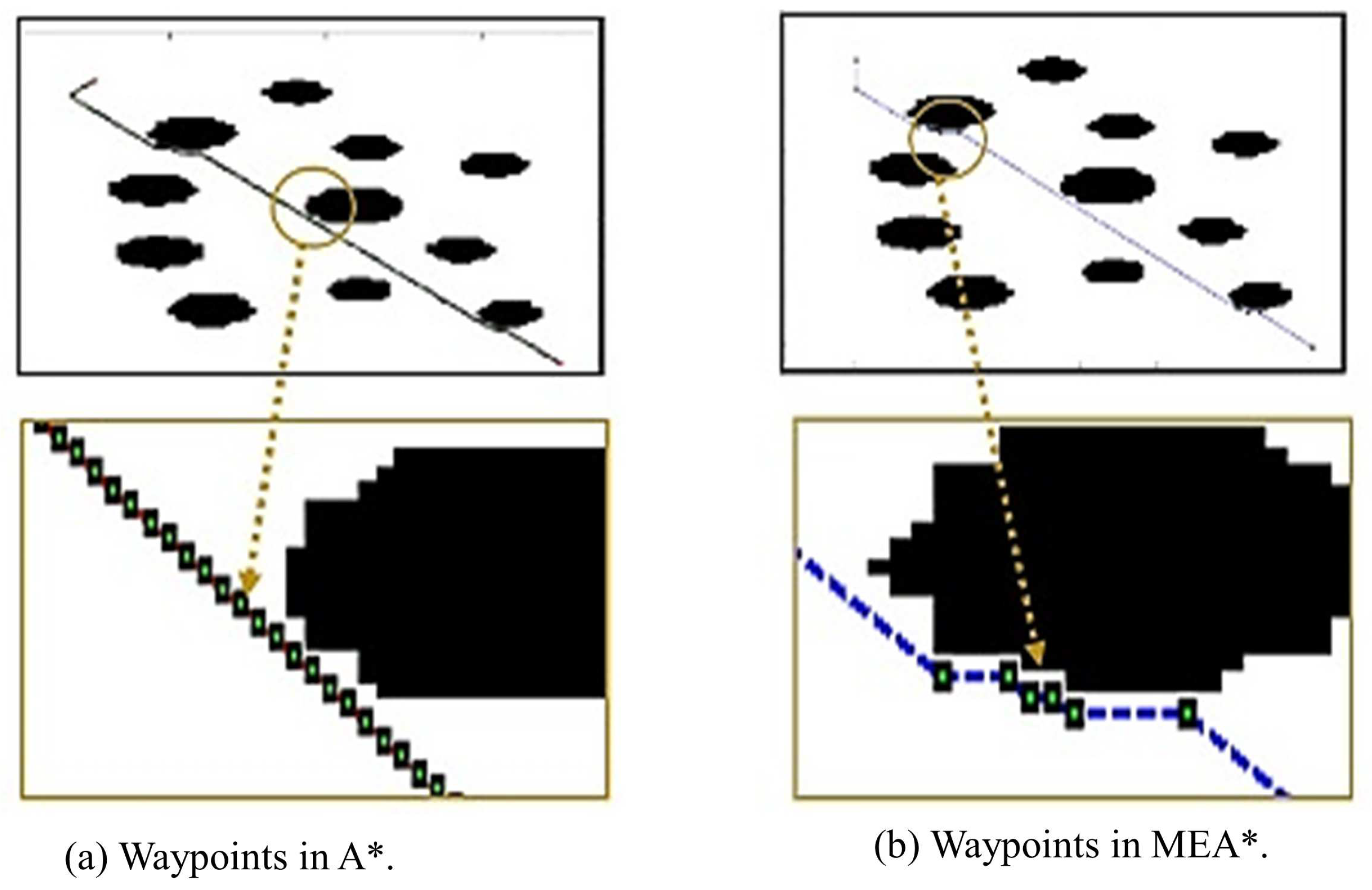
3.1. MEA* Algorithm
| Algorithm 1: [20]. |
 |
| Algorithm 2: path ← postSmoothPath(pathFound) [20]. |
 |
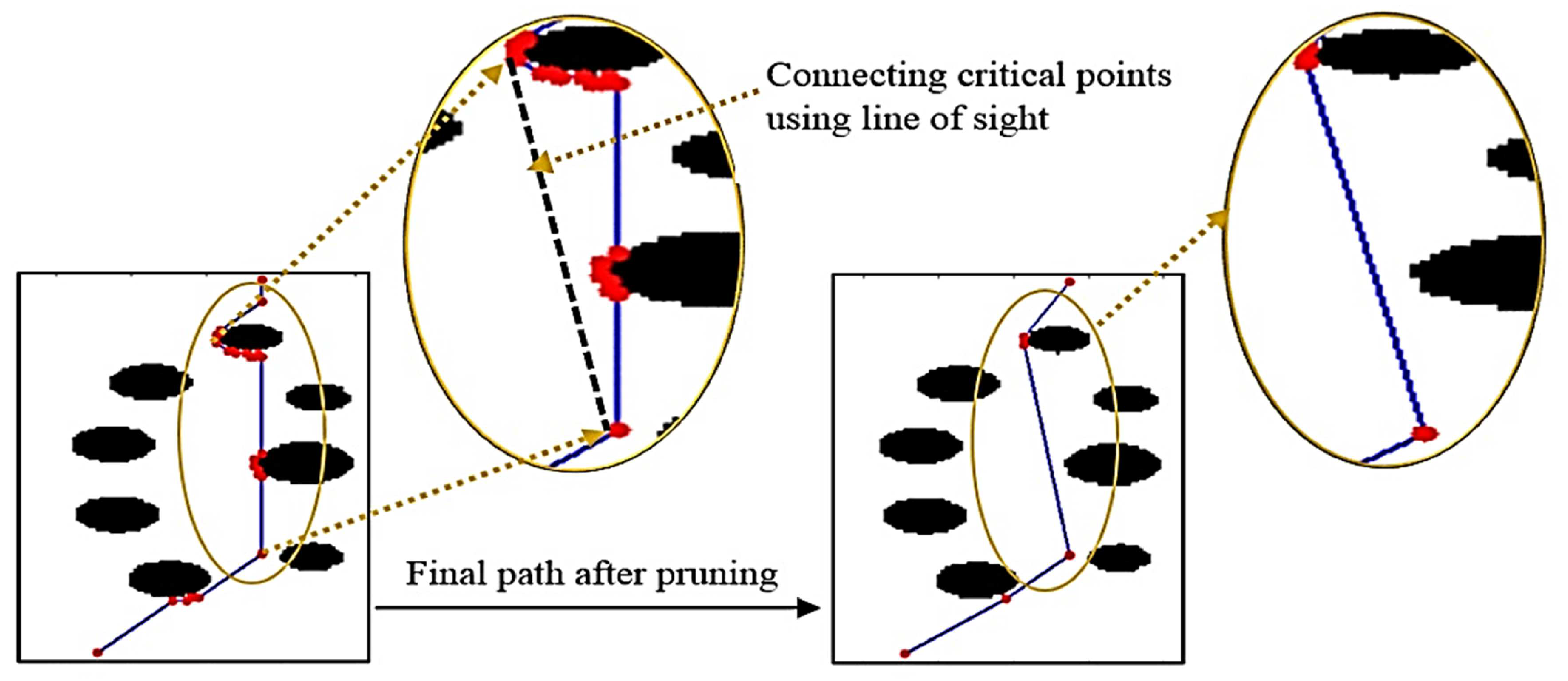
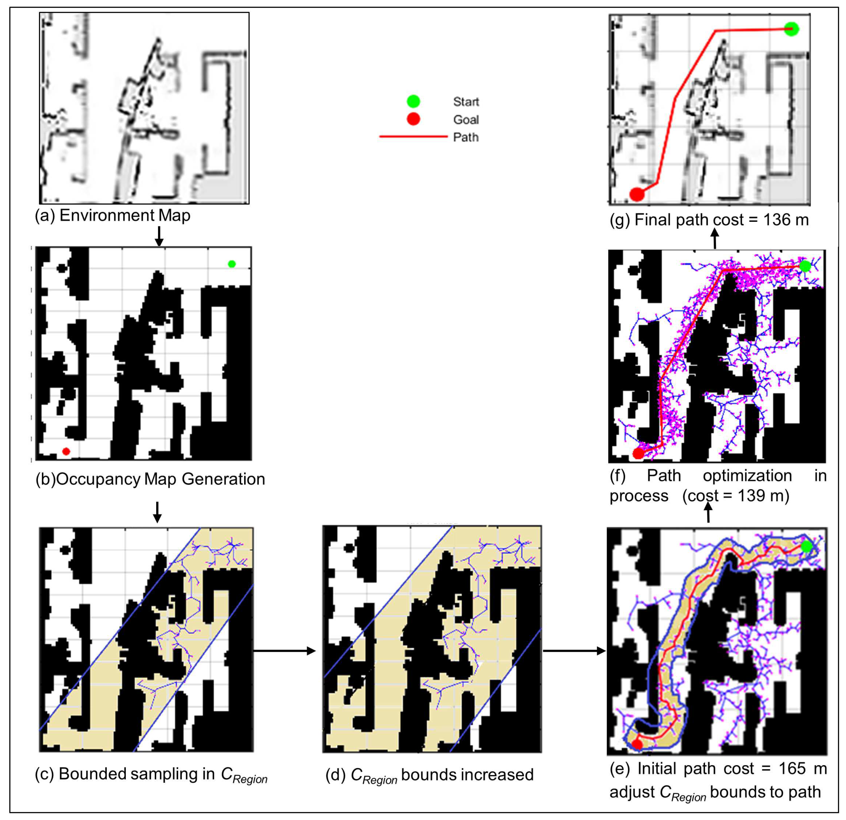
3.2. RRT*-AB Algorithm
| Algorithm 3: [12]. |
 |
3.3. Complexity Analysis
3.4. Data Set
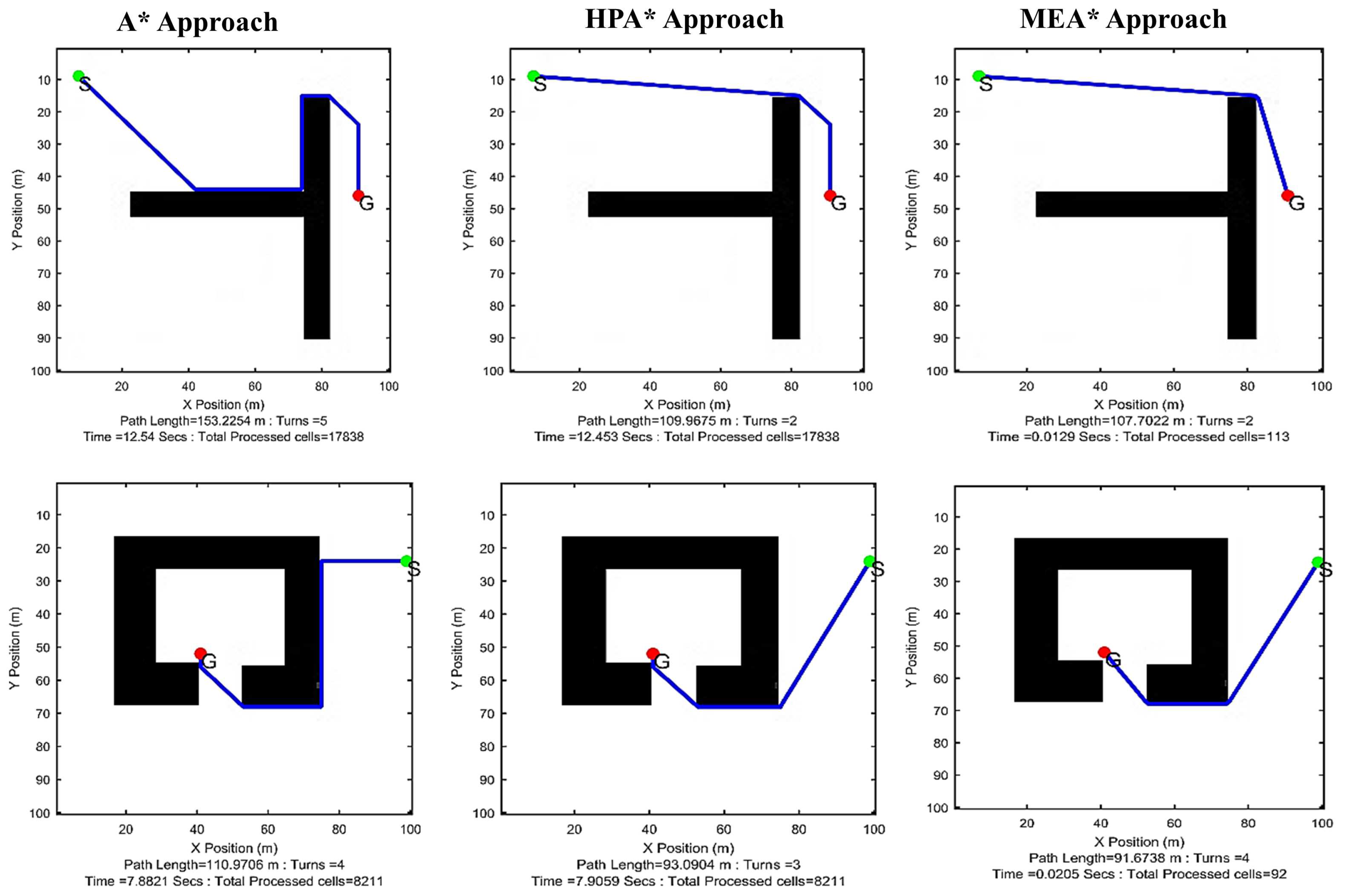
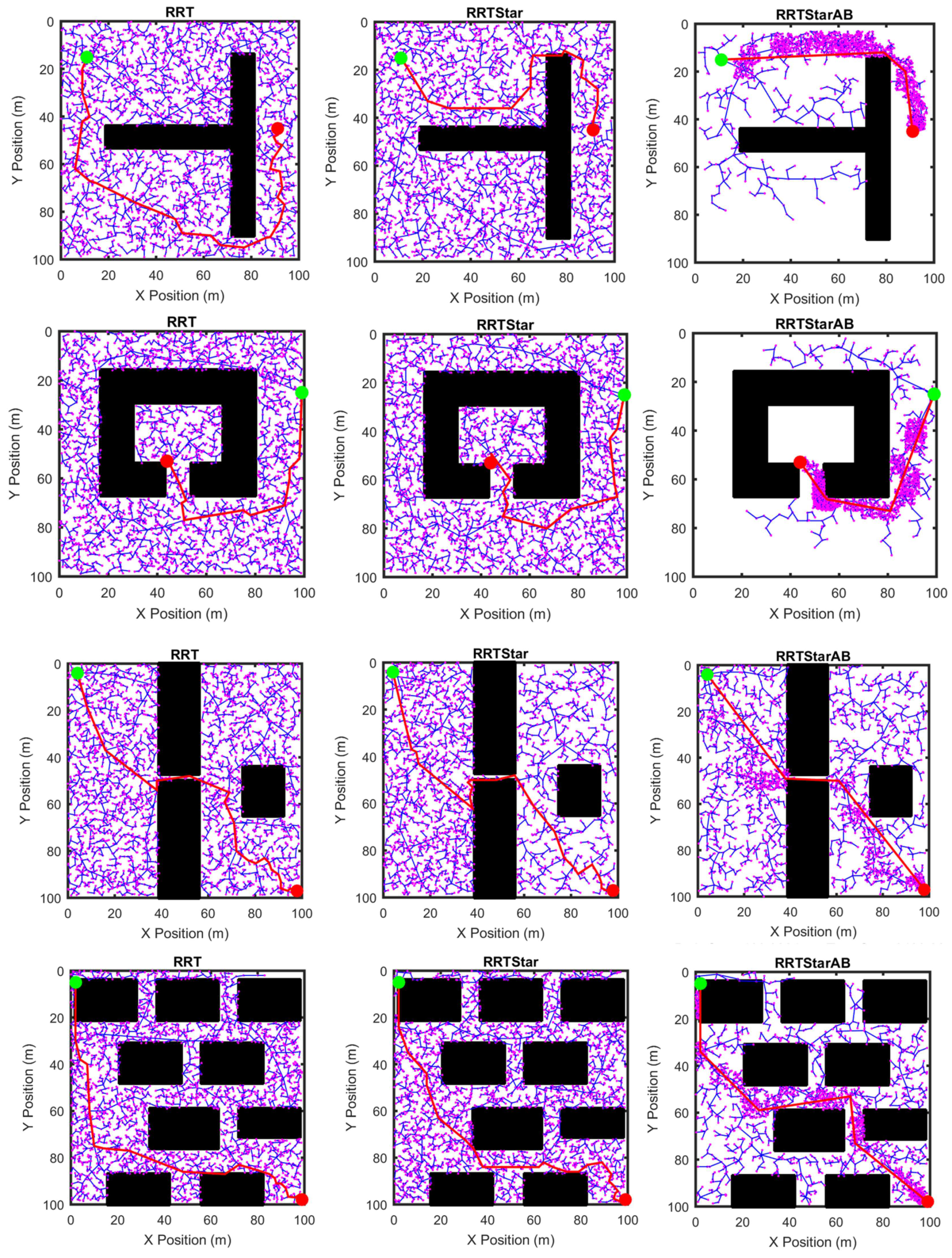
- Simple Structured Environment: M1 is the case of a structured environment map such as a turning passage.
- Concave Structured Environment: M2 represents an environment with concave shape obstacle.
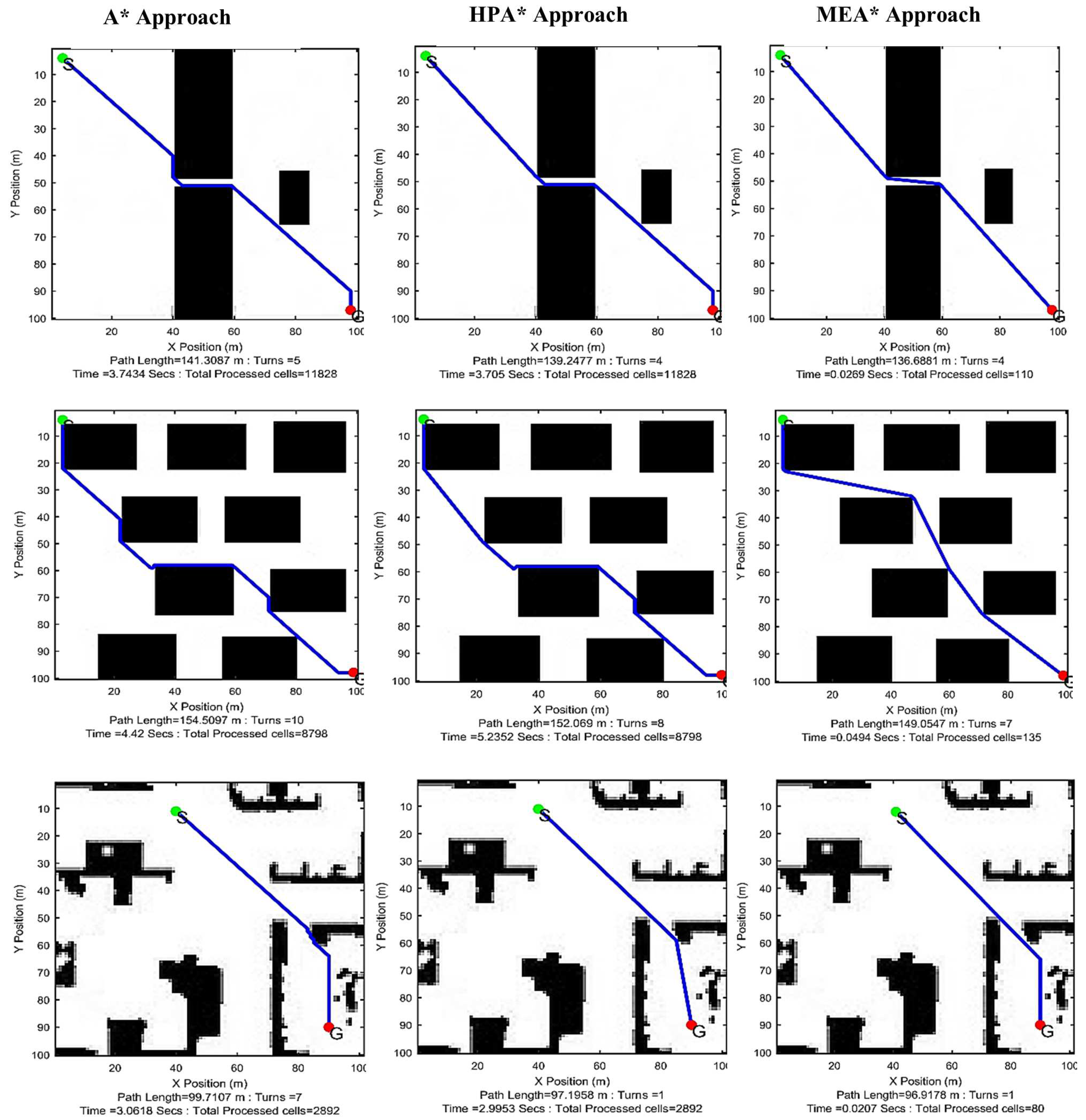
- Narrow Structured Environment: M3 is the case of a narrow structured environment.
- Dense Structured Environment: M4 signifies a highly dense environment.
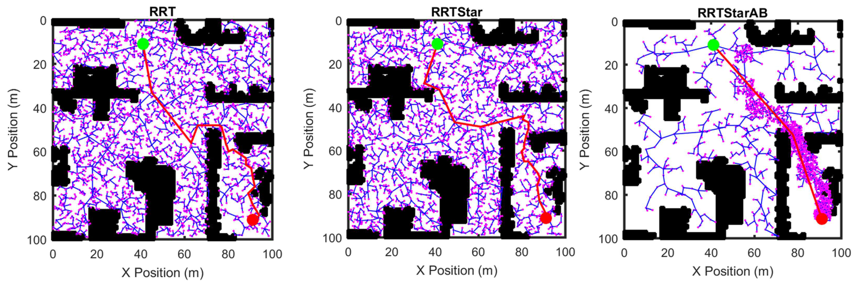
- Complex Unstructured Environment: M5 is an example of a complex indoor and unstructured scenario.
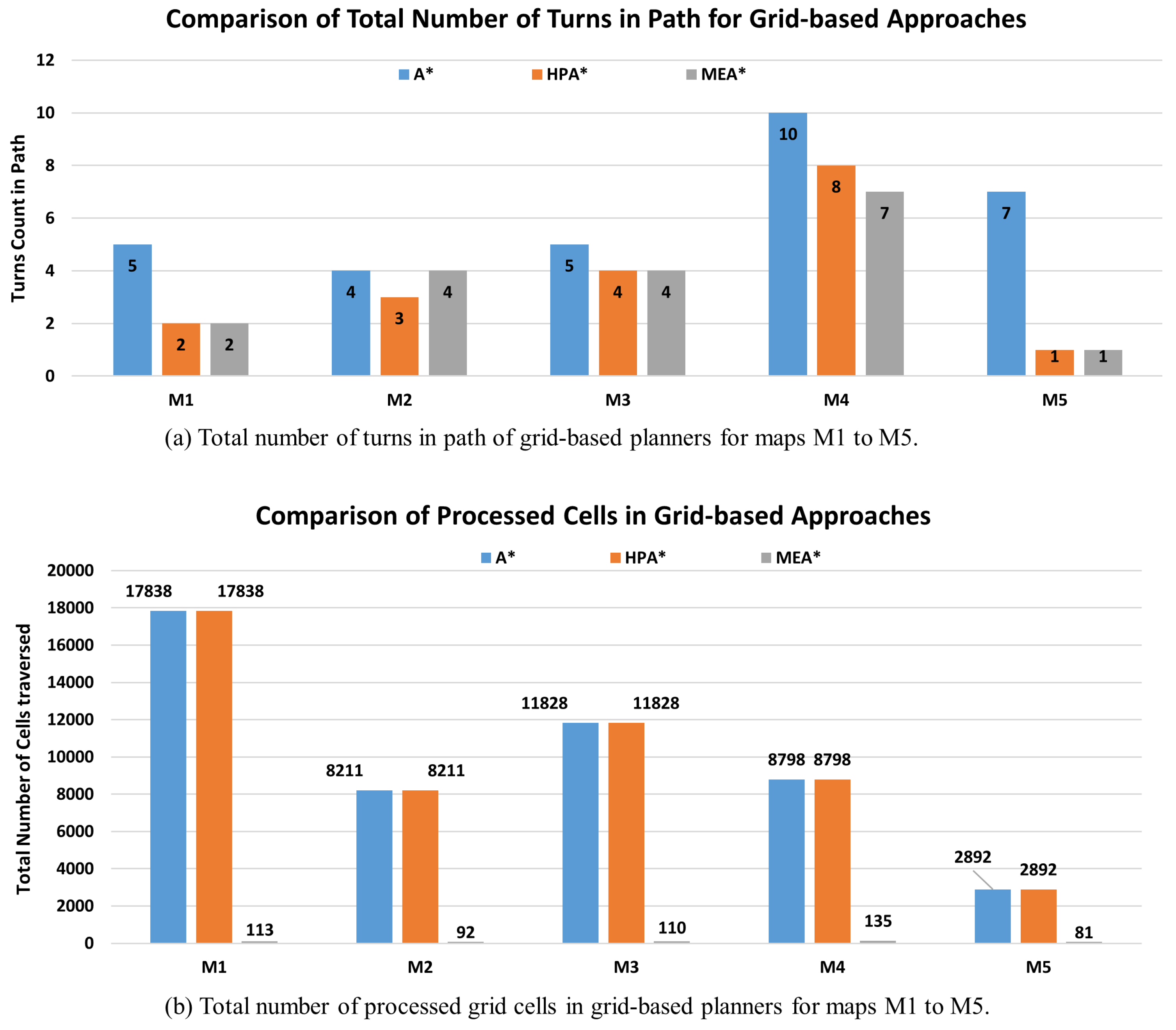
3.5. Performance Metrics
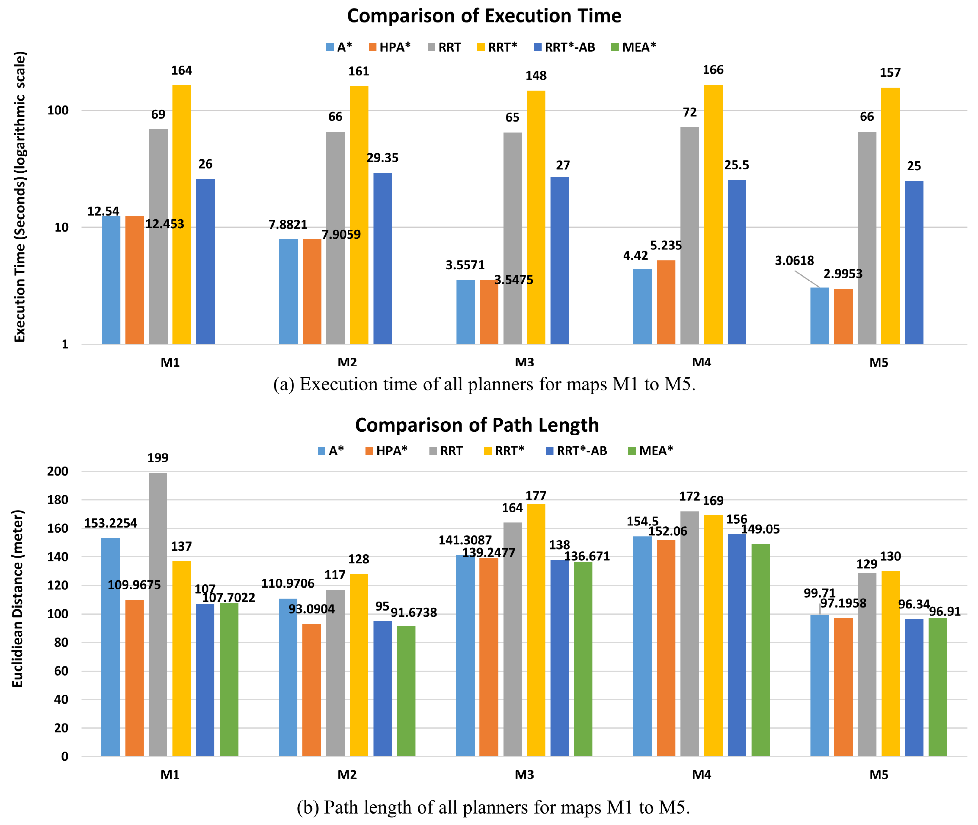
- Total Path Length: The total coverage length determines the total operational time required to perform the coverage task and the total energy consumption of the mobile robot. The path- planning algorithm is considered optimal if it generates the shortest path, thus leading to energy efficiency. Therefore, it is an important parameter for real-world solutions.
- Computational Time: The time required to compute the solution is preeminent for real-world applications. Hence, is a prominent efficiency indicator of the proposed approach.
- Memory Requirements: Memory requirements indicate the total number of vertices visited while performing the coverage task. This directly influences the total computational time required by the algorithm to find a solution.
4. Results
4.1. Comparison with Sampling-BASED Algorithms
4.2. Statistical Analysis
5. Conclusions
Author Contributions
Funding
Conflicts of Interest
Abbreviations
| MEA* | Memory-Efficient A* |
| RRT | Rapidly Exploring Random Tree |
| RRT* | Rapidly Exploring Random Tree Star |
| RRT*-AB | RRT*-Adjustable Bounds |
| UAV | Unmanned Aerial Vehicle |
| GA | Genetic Algorithm |
| PSO | Particle Swarm Optimization |
| ACO | Ant Colony Optimization |
| SBP | Sampling-Based Planning |
| IDA* | Iterative Deepening A* |
| FD* | Field D* |
| HPA* | Hierarchical A* |
| A*PS | A* Post Smoothing |
References
- Veeraswamy, A.; Amavasai, B. Optimal path planning using an improved A* algorithm for homeland security applications. In Proceedings of the International Conference on Artificial Intelligence and Applications, Innsbruck, Austria, 13–16 February 2006; ACTA Press: Anaheim, CA, USA; pp. 50–55. [Google Scholar]
- Kuwata, Y.; Elfes, A.; Maimone, M.; Howard, A.; Pivtoraiko, M.; Howard, T.M.; Stoica, A. Path Planning Challenges for Planetary Robots. IEEE Intell. Robot. Syst. 2008, 22–27. [Google Scholar] [CrossRef]
- Noreen, I.; Khan, A.; Habib, Z. Optimal Path Planning using RRT* Based Approaches: A Survey and Future Directions. Int. J. Adv. Comput. Sci. Appl. (IJACSA) 2016, 7, 97–107. [Google Scholar] [CrossRef]
- Alejo, D.; Cobano, J.A.; Heredia, G.; Martinez-de Dios, J.R.; Ollero, A. Efficient Trajectory Planning for WSN Data Collection with Multiple UAVs. In Cooperative Robots and Sensor Networks; Springer International Publishing: New York, NY, USA, 2015; Volume 604, pp. 53–75. [Google Scholar]
- Ahmidi, N.; Hager, G.D.; Ishii, L.; Gallia, G.L.; Ishii, M. Robotic Path Planning for Surgeon Skill Evaluation in Minimally-Invasive Sinus Surgery. In Proceedings of the 15th International Conference on Medical Image Computing and Computer-Assisted Intervention, Nice, France, 1–5 October 2012; pp. 471–478. [Google Scholar]
- LaValle, S.M. Planning Algorithms; Cambridge University Press: Cambridge, UK, 2006. [Google Scholar]
- Canny, J.; Rege, A.; Reif, J. An Exact Algorithm for Kinodynamic Planning in the Plane. Discret. Comput. Geom. 1991, 6, 461–484. [Google Scholar] [CrossRef]
- Guernane, R.; Achour, N. Generating optimized paths for motion planning. Robot. Auton. Syst. 2011, 59, 789–800. [Google Scholar] [CrossRef]
- Zhang, H.Y.; Lin, W.M.; Chen, A.X. Path Planning for the Mobile Robot: A Review. Symmetry 2018, 10, 450. [Google Scholar] [CrossRef]
- Arora, T.; Gigras, Y.; Arora, V. Robotic Path Planning using Genetic Algorithm in Dynamic Environment. Int. J. Comput. Appl. 2014, 89, 8–12. [Google Scholar] [CrossRef]
- Liang, J.H.; Lee, C.H. Efficient Collision-free Path-planning of Multiple Mobile Robots System using Efficient Artificial Bee Colony Algorithm. Adv. Eng. Softw. 2015, 79, 47–56. [Google Scholar] [CrossRef]
- Noreen, I.; Khan, A.; Habib, Z. Optimal Path Planning using RRT*-Adjustable Bounds. Intell. Serv. Robot. 2018, 11, 41–52. [Google Scholar] [CrossRef]
- Noreen, I.; Khan, A.; Habib, Z. A Comparison of RRT, RRT* and RRT*-Smart Path Planning Algorithms. Int. J. Comput. Sci. Netw. Secur. 2016, 16, 20–27. [Google Scholar]
- Kormushev, P.; Calinon, S.; Caldwe, D.G. Reinforcement Learning in Robotics: Applications and Real-World Challenges. Robot. Auton. Syst. 2013, 2, 122–148. [Google Scholar] [CrossRef] [Green Version]
- Luviano-Cruz, D.; Garcia-Luna, F.; Pérez-Domínguez, L.; Gadi, S.K. Multi-Agent Reinforcement Learning Using Linear Fuzzy Model Applied to Cooperative Mobile Robots. Symmetry 2018, 10, 461. [Google Scholar] [CrossRef]
- Karaman, S.; Frazzoli, E. Sampling-based Algorithms for Optimal Motion Planning. Int. J. Robot. Res. 2011, 30, 846–894. [Google Scholar] [CrossRef]
- Hart, P.E.; Nilsson, N.J.; Raphael, B. A Formal Basis for the Heuristic Determination of Minimum Cost Paths. IEEE Trans. Syst. Sci. Cybern. 1968, 4, 100–107. [Google Scholar] [CrossRef]
- Daniel, K.; Nash, A.; Koenig, S. Theta Any-Angle Path Planning on Grids. J. Artif. Intell. Res. 2010, 39, 533–579. [Google Scholar] [CrossRef]
- Conlter, R.C. Implementation of the Pure Pursuit Path Tracking Algorithm; Report; The Robotics Institute, Camegie Mellon University: Pittsburgh, PA, USA, 1992. [Google Scholar]
- Noreen, I.; Khan, A.; Habib, Z. Optimal Path Planning using Memory Efficient A*. In Proceedings of the IEEE International Conference on Frontiers of Information Technology, Islamabad, Pakistan, 19–21 December 2016; pp. 142–146. [Google Scholar]
- Goerzen, C.; Kong, Z.; Mettler, B. A Survey of Motion Planning Algorithms from the Perspective of Autonomous UAV Guidance. J. Intell. Robot. Syst. 2009, 57, 65–100. [Google Scholar] [CrossRef]
- Dijkstra, E.W. A Note on Two Problems in Connexion with Graphs. Numer. Math. 1959, 1, 269–271. [Google Scholar] [CrossRef]
- Noto, M.; Univ, K.; Sato, H. A Method for the Shortest Path Search by Extended Dijkstra Algorithm. In Proceedings of the IEEE International Conference on Systems, Man, and Cybernetics, Nashville, TN, USA, 8–11 October 2000; Volume 3, pp. 2316–2320. [Google Scholar]
- Botea, A.; Muller, M.; Schaeffer, J. Near Optimal Hierarchical Path-Finding. J. Game Dev. 2004, 1, 1–30. [Google Scholar]
- Warren, C.W. Fast path planning using modified A* method. In Proceedings of the IEEE International Conference on Robotics and Automation, Atlanta, GA, USA, 2–6 May 1993. [Google Scholar]
- Zhang, X.; Chen, J.; Xin, B. Path Planning for Unmanned Aerial Vehicles in Surveillance Tasks Under Wind Fields. J. Cent. South Univ. 2014, 21, 3079–3091. [Google Scholar] [CrossRef]
- Koenig, S.; Likhachev, M.; Furcy, D. Lifelong Planning A*. Artif. Intell. 2004, 155, 93–146. [Google Scholar] [CrossRef]
- Korf, R.E. Depth-first iterative-deepening. Artif. Intell. 1985, 27, 97–109. [Google Scholar] [CrossRef]
- Ferguson, D.; Kalra, N.; Stentz, A. Replanning with RRTs. In Proceedings of the IEEE International Conference on Robotics and Automation, Orlando, FL, USA, 15–19 May 2006. [Google Scholar]
- LaValle, S.M. Rapidly-Exploring Random Trees: A New Tool for Path Planning; Technical Report; Computer Science Dept., Iowa State University: Ames, IA, USA, 1998. [Google Scholar]
- Nasir, J.; Islam, F.; Malik, U.; Ayaz, Y.; Hasan, O.; Khan, M.; Saeed, M. RRT*-SMART: A Rapid Convergence Implementation of RRT*. Int. J. Adv. Robot. Syst. 2013, 10, 1–12. [Google Scholar] [CrossRef]
- Stachniss, C. Robotics Datasets, University of Freiberg, 2016. Available online: http://www2.informatik.uni-freiburg.de/~stachnis/datasets.html (accessed on 14 June 2019).
- Qureshi, A.H.; Ayaz, Y. Intelligent Bidirectional Rapidly-exploring Random Trees for Optimal Motion Planning in Complex Cluttered Environments. Robot. Auton. Syst. 2015, 68, 1–11. [Google Scholar] [CrossRef]


| Map | A* | HPA* | RRT | RRT* | RRT*-AB | MEA* |
|---|---|---|---|---|---|---|
| M1 (Simple Case) | 12.54 | 12.453 | 69 | 164 | 26 | 0.0129 |
| M2 (Concave Case) | 7.8821 | 7.9059 | 66 | 161 | 29.35 | 0.0205 |
| M3 (Narrow Case) | 3.5571 | 3.5475 | 65 | 148 | 27 | 0.0094 |
| M4 (Dense Case) | 4.42 | 5.235 | 72 | 166 | 25.5 | 0.0494 |
| M5 (Complex Unstructured Case) | 3.0618 | 2.9953 | 66 | 157 | 25 | 0.0207 |
| Total | 31.461 | 32.1367 | 338 | 796 | 132.85 | 0.1129 |
| Mean | 6.2922 | 6.42734 | 67.6 | 159.2 | 26.57 | 0.02258 |
| Std Dev | 3.9681 | 3.8726 | 2.8809 | 7.1203 | 1.7210 | 0.0157 |
| Std Dev Err | 1.7746 | 1.7318 | 1.2884 | 3.1843 | 0.7696 | 0.0071 |
| Map | A* | HPA* | RRT | RRT* | RRT*-AB | MEA* |
|---|---|---|---|---|---|---|
| M1 (Simple Case) | 153.23 | 109.97 | 199 | 137 | 107 | 107.70 |
| M2 (Concave Case) | 110.97 | 93.09 | 117 | 128 | 95 | 91.67 |
| M3 (Narrow Case) | 141.31 | 139.25 | 164 | 177 | 138 | 136.67 |
| M4 (Dense Case) | 154.50 | 152.06 | 172 | 169 | 156 | 149.05 |
| M5 (Complex Un-structure Case) | 99.71 | 97.20 | 129 | 130 | 96.34 | 96.91 |
| Total | 659.7147 | 591.5614 | 781 | 741 | 592.34 | 582.007 |
| Mean | 131.94294 | 118.31228 | 156.2 | 148.2 | 118.468 | 116.4014 |
| Std Dev | 25.1410 | 26.1193 | 33.2370 | 23.0586 | 27.2124 | 25.2182 |
| Std Dev Err | 11.2434 | 11.6809 | 14.8640 | 10.3121 | 12.1697 | 11.2779 |
© 2019 by the authors. Licensee MDPI, Basel, Switzerland. This article is an open access article distributed under the terms and conditions of the Creative Commons Attribution (CC BY) license (http://creativecommons.org/licenses/by/4.0/).
Share and Cite
Noreen, I.; Khan, A.; Asghar, K.; Habib, Z. A Path-Planning Performance Comparison of RRT*-AB with MEA* in a 2-Dimensional Environment. Symmetry 2019, 11, 945. https://doi.org/10.3390/sym11070945
Noreen I, Khan A, Asghar K, Habib Z. A Path-Planning Performance Comparison of RRT*-AB with MEA* in a 2-Dimensional Environment. Symmetry. 2019; 11(7):945. https://doi.org/10.3390/sym11070945
Chicago/Turabian StyleNoreen, Iram, Amna Khan, Khurshid Asghar, and Zulfiqar Habib. 2019. "A Path-Planning Performance Comparison of RRT*-AB with MEA* in a 2-Dimensional Environment" Symmetry 11, no. 7: 945. https://doi.org/10.3390/sym11070945