Article

Multilevel and Multiscale Deep Neural Network for Retinal Blood Vessel Segmentation

by
Pearl Mary Samuel
and
Thanikaiselvan Veeramalai
*
School of Electronics Engineering, Vellore Institute of Technology, Vellore 632014, India
*
Author to whom correspondence should be addressed.
Symmetry 2019, 11(7), 946; https://doi.org/10.3390/sym11070946
Submission received: 21 May 2019 / Revised: 13 July 2019 / Accepted: 17 July 2019 / Published: 22 July 2019
(This article belongs to the Special Issue Symmetry and Asymmetry in Computational Biology and Bioinformatics)

Abstract

:
Retinal blood vessel segmentation influences a lot of blood vessel-related disorders such as diabetic retinopathy, hypertension, cardiovascular and cerebrovascular disorders, etc. It is found that vessel segmentation using a convolutional neural network (CNN) showed increased accuracy in feature extraction and vessel segmentation compared to the classical segmentation algorithms. CNN does not need any artificial handcrafted features to train the network. In the proposed deep neural network (DNN), a better pre-processing technique and multilevel/multiscale deep supervision (DS) layers are being incorporated for proper segmentation of retinal blood vessels. From the first four layers of the VGG-16 model, multilevel/multiscale deep supervision layers are formed by convolving vessel-specific Gaussian convolutions with two different scale initializations. These layers output the activation maps that are capable to learn vessel-specific features at multiple scales, levels, and depth. Furthermore, the receptive field of these maps is increased to obtain the symmetric feature maps that provide the refined blood vessel probability map. This map is completely free from the optic disc, boundaries, and non-vessel background. The segmented results are tested on Digital Retinal Images for Vessel Extraction (DRIVE), STructured Analysis of the Retina (STARE), High-Resolution Fundus (HRF), and real-world retinal datasets to evaluate its performance. This proposed model achieves better sensitivity values of 0.8282, 0.8979 and 0.8655 in DRIVE, STARE and HRF datasets with acceptable specificity and accuracy performance metrics.

1. Introduction

Retinal blood vessel disorders hinder the vision of diabetic patients. With an unusual increase in the number of patients with vision impairments [1], the need for periodic eye checkups has risen tremendously. Due to there being very few ophthalmologists, screening each and every eye is difficult. Hence automatic supervised procedures are a boon in this particular field [2,3]. For the past two decades, researchers have been working on the segmentation of blood vessels to screen out many diseases that influence the blood vessels. Tortuous blood vessels in the retina confirm the presence of diabetic retinopathy (DR) [4], hypertension, cerebral vessel disorders [5], ischemic heart disease, and stroke. Neovascularization [6], a severe stage of DR, causes more new blood vessels to grow. These vessels lack the bifurcation pattern, rigidness, and integrity that bleed with fewer traumas. Hypertensive retinopathy is distinguished by arteriovenous crossings and artery width [7]. Retinal telangiectasia [8], a macular disease causes the tiny blood vessels around the fovea to leak or become dilated. Also, the arteriovenous ratio and crossing provide information on a lot of vessel-related disorders [9]. Moreover, the vessels are removed for glaucoma detection [10,11,12].
Segmentation of blood vessel structures has improved greatly with a lot of emerging approaches [13]. Morphological processing segments the blood vessel structures but the combination with other methods is necessary to obtain accurate results [14]. Matched filtering approaches are unable to segment vessels at the region of pathologies, central reflex and low contrast [15,16,17,18,19]. Information obtained from multiple scales was able to segment vessels but it could not detect low contrast thin vessels [20,21,22,23]. Region growing methods also proved to be a useful technique in vessel segmentation but expertise is needed in vessel seed point setting and in the formulation of a stopping rule [24,25,26]. Over-segmentation occurs when the input is noisy and is also a hugely time-consuming method. Active contour model-based approaches are independent and self-adjusting in their search and their accuracy depends on contour fitting [27,28,29]. Pattern recognition-based methods include both unsupervised and supervised algorithms to accurately segment the vessels. Although unsupervised methods do not need prior knowledge about the segmentation and are fast to run [30,31], it takes time to interpret the results correctly. Supervised methods require a lot of features and expertise to accurately segment the blood vessels [32,33,34,35,36,37]. Supervised learning algorithms based on deep convolutional neural networks (CNN) show utmost robustness and efficiency in segmenting the blood vessels. Unlike any supervised approach which relies on artificial handcrafted features, the deep neural network (DNN) is capable of learning the features by itself with the help of convolutional layers.
In DNN, during the training phase, the network rather learns from scratch or uses the concept of transfer learning to restructure the existing CNN models and fine-tune them for more relevant applications. A five-stage DNN using autoencoder was able to transform an input RGB retinal patch into blood vessel map by providing predictions at each pixel in the patch [38]. It segments even fine vessels and works perfectly in the presence of pathologies. Liskowski and Krawiec trained a CNN using the fundus image patches that are preprocessed using zero-phase whitening, global contrast normalization, and gamma corrections [39]. Testing on the retinal datasets showed reduced vessel misclassification and central vessel reflex problems. A patch input-based DNN with a probabilistic tracking framework is proposed to segment the blood vessels [40]. It provides more information about the vessel tree.
With the patch image as input to the CNN, training and prediction efficiency is degraded, but with the fully convolutional neural network (FCN) where the entire image is used for training and prediction, speed and efficiency are increased. FCN inspired by holistically-nested edge detection (HED) [41], is combined with fully connected conditional random fields (CRF) to obtain binary vessel segmentation [42]. Similarly, Maninis et al. proposed a deeply supervised FCN that performs both optic disc and retinal blood vessel segmentation efficiently [43]. Mo and Zhang proposed a deeply supervised multilevel FCN for segmenting the blood vessels more robustly [44]. Zhou et al. used pairwise features learned from fine vessels together with the unary features from patch input CNN as a feature extractor [45]. The extracted features are given to the dense CRF for vessel segmentation. A label-free DNN was proposed to avoid the ground truth labels for training [46]. Here, with prior knowledge of the domain, an artificial dataset was developed with basic line segments. Another efficient three-stage network model is proposed that segments the thick and thin vessels separately and further fuses them to get complete vessel segmentation [47]. This segmentation performs better but it has a complex, long structure which takes a lot of time and effort.
For appropriate blood vessel segmentation, this paper uses a DNN with the following contributions.
  • A better pre-processing approach that highlights the blood vessels;
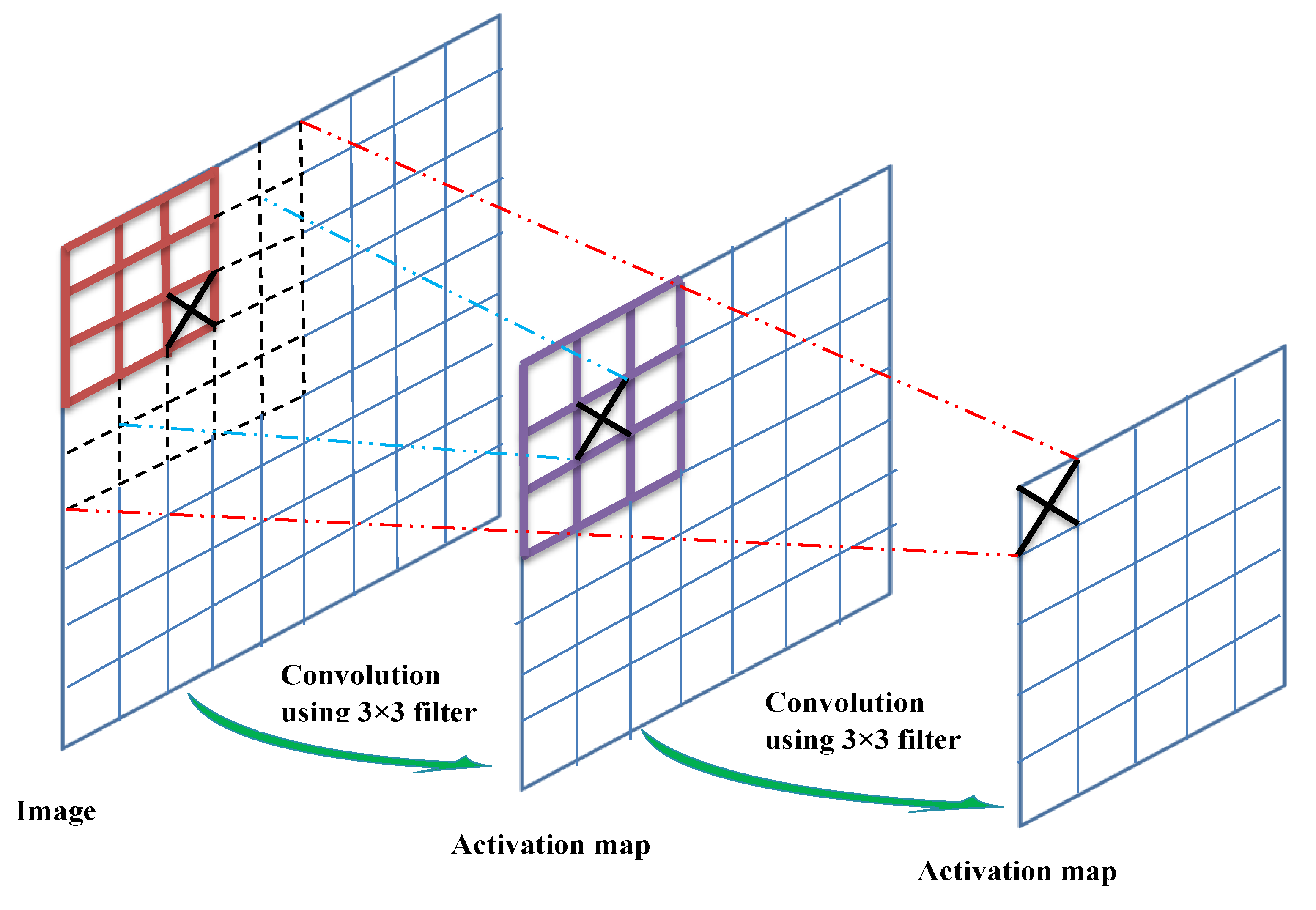
  • Incorporation of multilevel and multiscale deep supervision (DS) networks that can dive deep into the final layers of the four convolutional layers with two different scale initializations i.e., 0.001 and 0.0002;
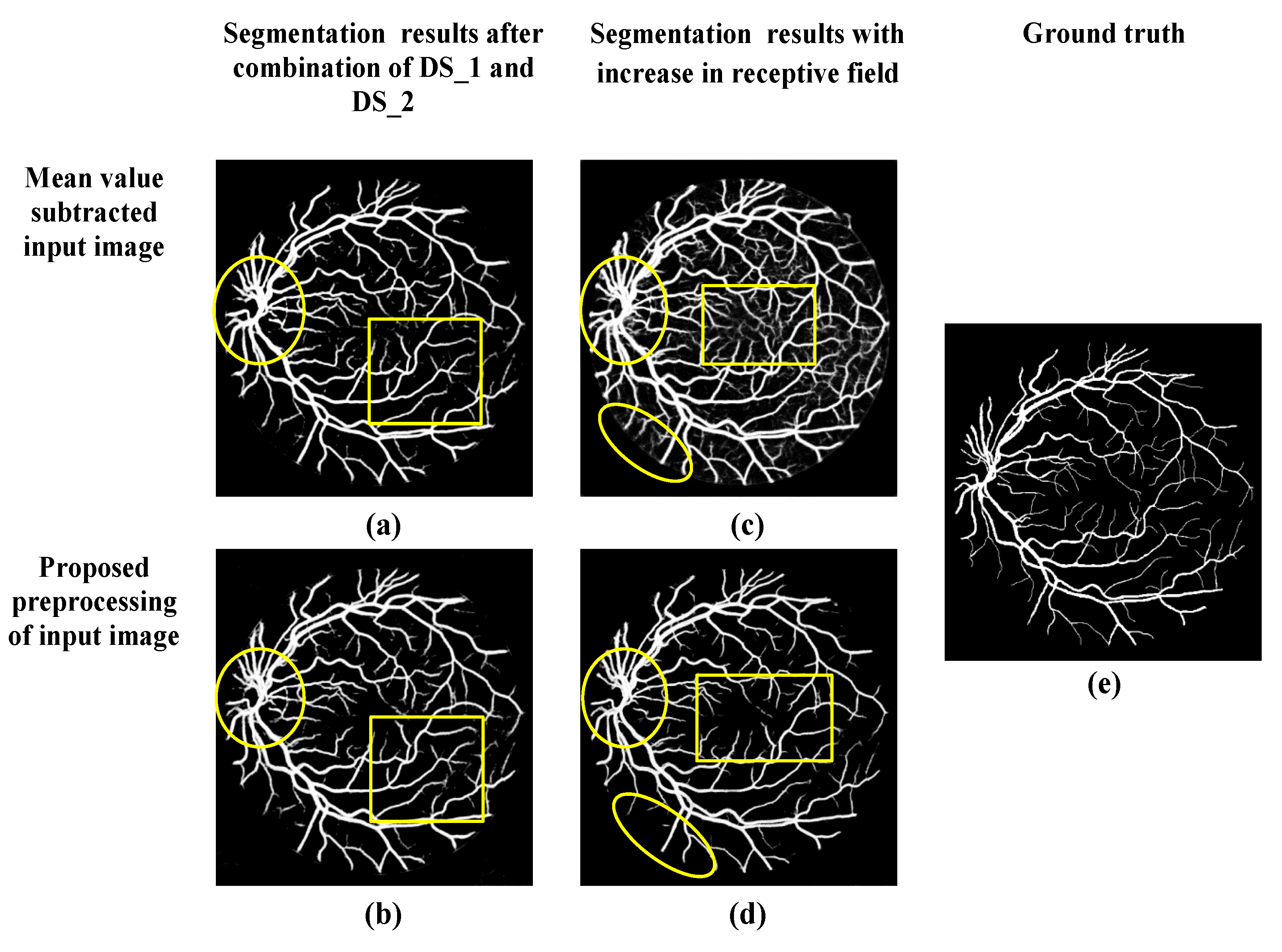
  • Furthermore, the receptive field of this multilevel and multiscale deep supervision (DS) network is increased to refine and localize the blood vessels. Therefore, the probability map obtained consists clearly of blood vessels with fewer false predictions.
The following Section 2 provides the datasets and the methodologies used. Section 3 provides the results obtained and validation of the proposed DNN model. Section 4 discusses the proposed model, results and explains its future scope. Section 5 ends with the conclusion.

2. Materials and Methods

The proposed network is trained using the images in the Digital Retinal Images for Vessel Extraction (DRIVE) [48] and STructured Analysis of the Retina (STARE) [49] retinal datasets. The trained network is tested using the images provided in the DRIVE, STARE, High-Resolution Fundus (HRF) [50] and real-world datasets. DRIVE dataset has been isolated into test and training set, both containing 20 images of size 565 × 584 with its ground truth. The STARE dataset contains 20 images of size 700 × 605 for blood vessel segmentation along with its ground truth. Therefore, 10 images are used for training and the remainder for testing. For additional justification of the proposed model, the proposed DNN is also tested on HRF. It consists of 15 retinal fundus images obtained from Diabetic Retinopathy patients together with its vessel segmented ground truth images. Other than the common datasets, a real-world dataset obtained from Mulamoottil Eye Hospital, Kerala, India, is also used to test the robustness of the proposed DNN model.

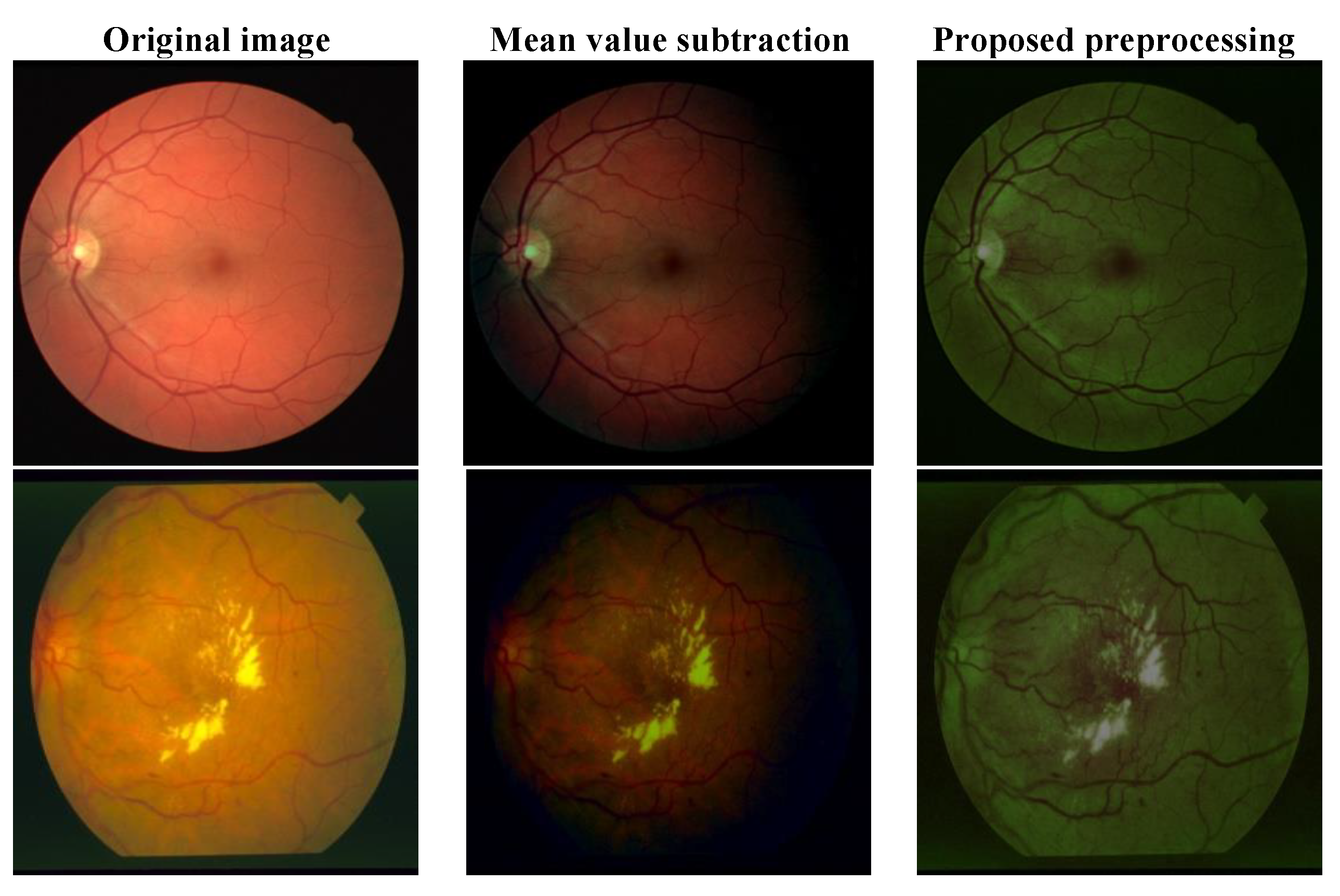
2.1. Proposed Preprocessing

Preprocessing generally makes the input more suitable for a specific application. Particularly in deep learning, preprocessing is undertaken to reduce the intensity range and highlight the region of interest. Reduction in intensity range reduces the computational overhead during training. The most common preprocessing technique used is mean value subtraction on the RGB plane for the entire input image dataset. Even though it reduces the intensity range, this method is not problem specific i.e., it darkens certain blood vessel regions in the dataset used for training. It can be seen clearly in Figure 1.
Hence, a new preprocessing method is implemented in this paper. Instead of using the conventional RGB plane, this paper uses three different planes. The first plane is the green plane. The second plane is obtained by applying Contrast Limited Adaptive Histogram Equalization (CLAHE) [51] on the green plane. The third plane is the linearized green plane after removing gamma corrections. Finally, the intensity range of all the three planes is reduced to half and concatenated to form the preprocessed image. As shown in Figure 1, the preprocessed images have almost half the intensity range and visibly highlighted blood vessel sections in comparison to mean value subtracted images. The superiority of this preprocessing approach is discussed in Section 4.

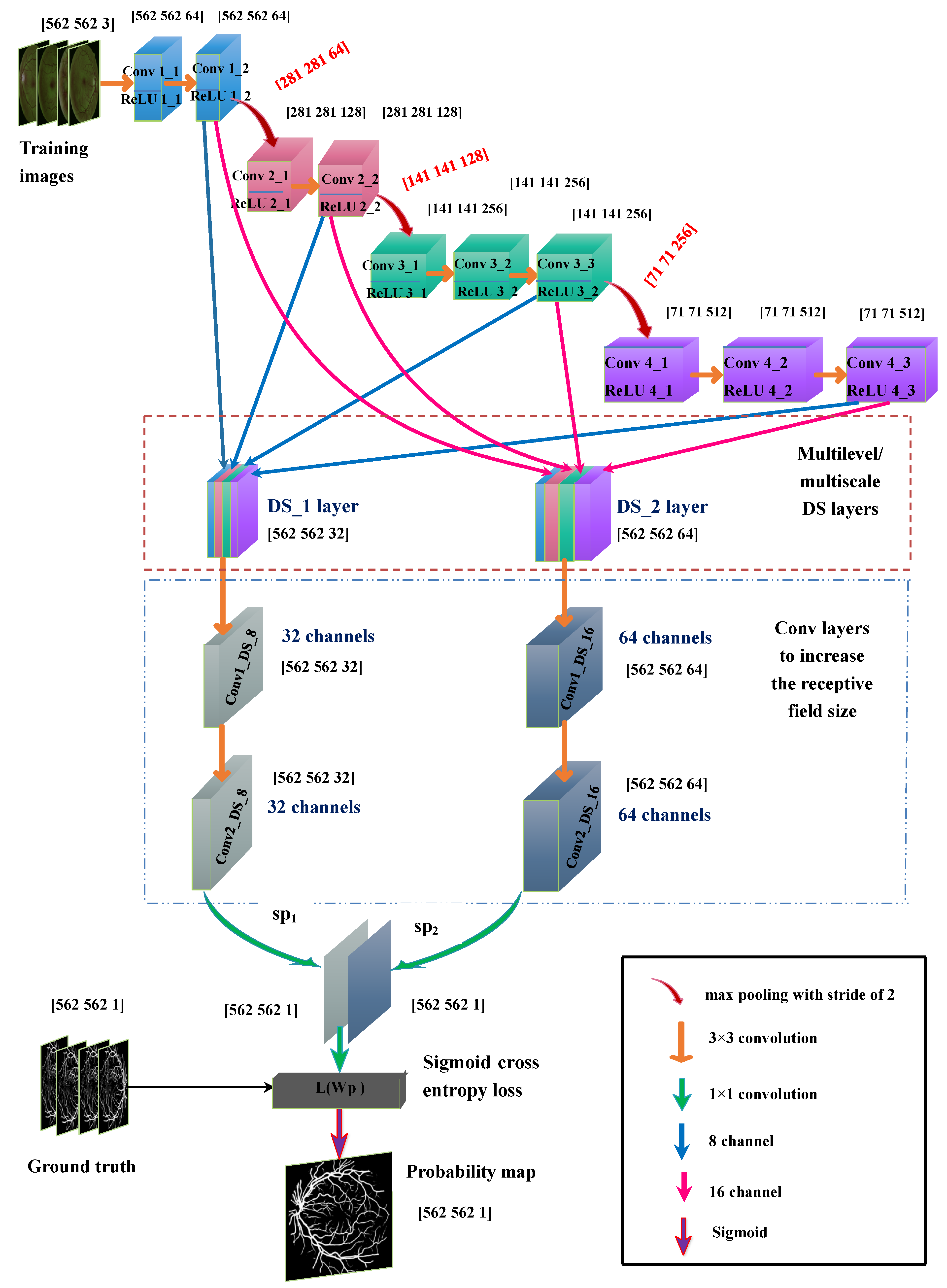
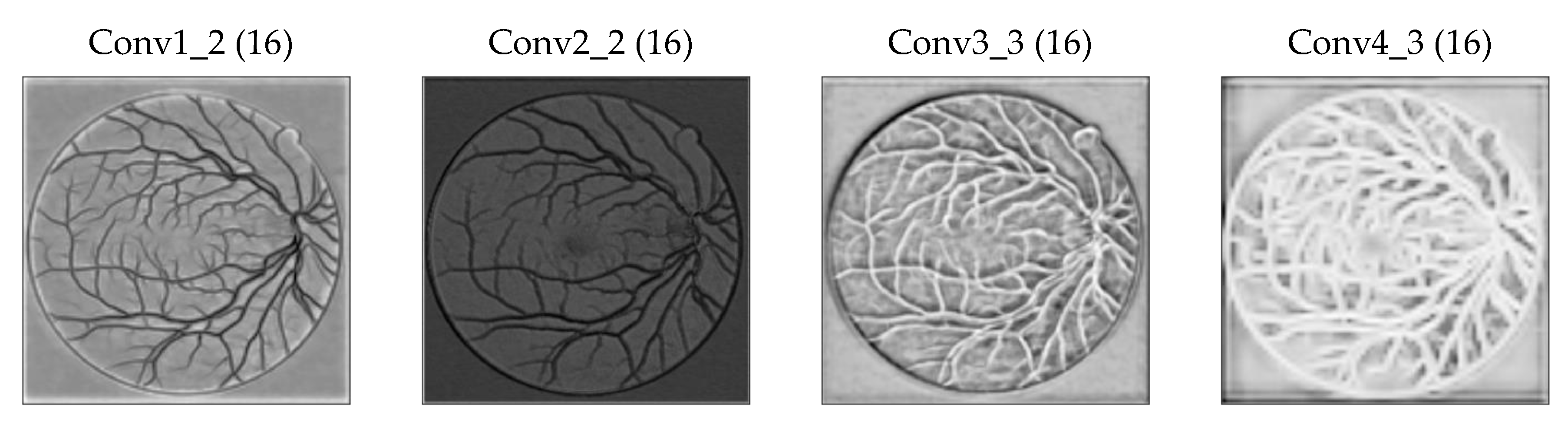
2.2. Proposed Multilevel/Multiscale Deep Neural Network (DNN)

In this paper, the proposed multilevel/multiscale DNN as depicted in Figure 2 performs a complete image–image regression.
Transfer learning helps to use the models pre-trained on a large scale dataset that is similar to the segmentation problem. Instead of developing a new model from scratch to solve a similar problem with a few input medical data, pre-trained model weights serve as a starting point. Transfer learning optimizes the learning process, saves time and improves the performance. Smaller learning rates are used to slowly vary the pre-trained model weights during training.
Due to the lack of an enormous amount of medical data for training, this DNN uses the initial 4 stages of VGG-16 that is already pre-trained on large-scale datasets for transfer learning [52]. Further, it is fine-tuned for blood vessel feature extraction. In this fine-tuning phase, multilevel and multiscale DS layers are incorporated to eliminate false segmentation by using deeply learned features from multiple levels/scales during training. Furthermore, the receptive field of view of DS layers is increased to localize vessel features and clearly segment the blood vessels. It is explained in more detail in the following subsections.

2.2.1. Base Network

The first four convolutional stages of a fully convolutional VGG-16 architecture are chosen as the initial stages of the proposed DNN model. These stages consist of the convolutional layers, rectifier linear units (ReLU) and the pooling layers. Since VGG-16 network learns fine to coarse features as it moves from one stage to another, more coarse features are not necessary for vessel segmentation. Hence the remaining convolution layers are excluded from the VGG-16 network.
Convolutional layers are the prominent building blocks in any DNN model. Here in Figure 2 which shows the entire block diagram of the proposed DNN model, these four convolutional blocks are depicted in blue, pink, green and purple. It consists of a set of learnable filters that extends throughout the depth of the input image. These set of filters will get activated to detect certain structures such as small edges in lower stages to patterns in the higher stages. Hence the network learns quite a number of features and produces feature maps at every filter output. Here, the filters in all the four stages of convolution layers consist of 3 × 3 kernel sizes with a padding of 1. The weights in these filters are initialized with Xavier initialization. First two stages consist of two separate convolution layers each and the remaining two stages consist of three separate convolution layers each. 64, 128, 256 and 512 are the number of feature maps from the first, second, third and last convolutional layers respectively. The width, height and depth parameters of the images and activation maps in the DNN are shown within brackets in Figure 2. The input image size is [562 562 3] i.e., width and height is 562 with a depth of 3.
ReLU is the activation function used at the end of every convolution layer. f(x) = max(0, x) is the activation function used by the neurons in the rectangular convolution grids. This adds non-linearity in the network which accelerates the convergence of stochastic gradient descent (SGD), unlike the conventional linear activation functions.
Max pooling layer downsample the activations obtained from the first three stages of convolutional layers. It is performed by applying a max filter with a stride of 2. It provides translational invariance as well as helps in reducing the computational overhead by reducing the learning parameter count. The image size is reduced to half in width and height as depicted in Figure 2. Max pooling yields better results than average pooling as discussed in [53]. For the identification of cerebral anomalies, a newer approach termed as stochastic pooling which takes additional activations in comparison to a maximum or average activations is proposed [54].

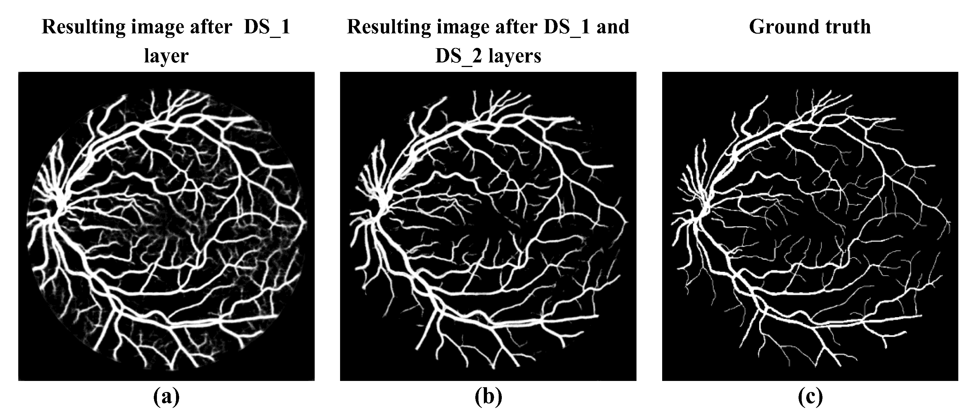
2.2.2. Deep Supervision (DS_1) Layer

All the four stages of the network contribute useful information about the blood vessels. Therefore, instead of focusing on the final stage activations, this paper aims to look deep into the activations in all four stages. It is evident that the blood vessels in the fundus image follow a Gaussian distribution as shown in Figure 3b. The width of the vessels generally varies from 0.5σ to 2σ values.
Therefore, the convolution layers with Gaussian kernels are used to extract useful blood vessel information. It has been observed that the selection of standard deviation values for the Gaussian kernel directly influence the segmentation of blood vessels. Choice of extreme values (0.1, 0.5, 1.0, 2, etc.) results in activation outputs that are exponentially increasing in magnitude eventually leading to the exploding gradient problem. This makes the network unable to train. On the contrary, the selection of too small values computes small gradients thereby making the training process very slow.
Therefore, the DS_1 layer is developed by performing eight vessel-specific convolutions on every stage/level of activations using a Gaussian kernel with an initial standard deviation initialization of 0.001. After initializing the first stage 8 vessel-specific convolutions with a standard deviation of 0.001, second, third and final stage standard deviations are set to 0.003, 0.005 and 0.007 values respectively. This combination of scales is found to be efficient in extracting the blood vessel features (vessels with varying sigma values i.e., varying vessel widths) using trial and error method. The kernel size is selected as 3 × 3 for all the eight Gaussian vessel- specific activations. This 3 × 3 kernel is sufficient to generate appropriate feature maps with reduced computational power.
As a result of performing convolutions on the final activations of all four stages, eight new vessel-specific feature maps are obtained from all four stages. In Figure 2 blue arrows depict the eight vessel-specific feature maps obtained from multiple levels. In order to depict the activations obtained from the chosen scales, the eight vessel-specific feature maps are individually combined by taking the argument of maxima of their output activations. It is shown in Figure 4. All four layer activations provide a portion of information about the varied blood vessel widths. In Figure 4, all the blood vessel sections standout in comparison to the background structures. Conv4_3 (8) is able to gather vessels of large widths in contrast to that of conv1_2 (8) which highlights small and thin vessel sections. The convolution layers learn fine to coarse information as they progress along the stages.
Therefore 8 × 4 = 32 vessel-specific activation maps are formed. These 32 feature maps are of varied size except those obtained from the first convolution layer because of bilinear interpolations. Hence, the remaining vessel-specific feature maps are cropped to the input image size and concatenated. This concatenation of 32 vessel-specific feature maps forms the multilevel/multiscale DS_1 layer. It contains blood vessel features obtained from multiple levels/scales.

2.2.3. Deep Supervision DS_2 Layer

Similar to the DS_1 layer, the DS_2 layer is introduced by changing the scale i.e., standard deviation initialization to 0.0002 in the Gaussian convolution. Here also convolution is performed on the four stages/levels but the number of the resulting activation map is set to 16. Since we need to cover all the blood vessels that are of varied size, we change the standard deviations to 0.0004, 0.0006 and 0.0008 for the second, third and fourth 16 vessel-specific Gaussian convolutions. Sixteen activation maps are selected as the output from every final convolution layer. Also since deep learning parameters are generally chosen in powers of 2, therefore DS_1 output activation is set to 8 (23) and DS_2 output activation is set to 16 (24). Also after experimenting with other combinations in powers of 2, it is found that this (8, 16) combination of deeply supervised activation outputs is efficient (with minimal output size, lesser computation, and fewer learning features).
Hence a total of 16 × 4 = 64 vessel-specific feature maps are obtained. These 64 feature maps are also cropped to the input image size and concatenated to form the second DS layer. The pink arrows in Figure 2 show the 16 vessel-specific activations obtained from the four convolutional layer stages. Similarly, the argument of maxima of the 16 vessel-specific activations from all the four convolution stages for the chosen scales is shown in Figure 5. The Gaussian kernels that perform the vessel-specific convolutions are kept to the nominal 3 × 3 sizes to reduce computational complexity and increase the efficiency. In Figure 5, the blood vessel regions are highlighted and the four 16 vessel-specific convolution covers all the blood vessels with varying widths. The vessel widths left out by DS_1 composition are picked up by DS_2 composition and vice versa.
Finally, a 32-feature map concatenation and a 64-feature map concatenation is the resulting outcome that has successfully learned blood vessel features by capturing all the possible blood vessel structures at multiple scales and levels. Therefore, this DS_1 and DS_2 combination can be seen as multilevel/multiscale DS layers capable to deeply learn the blood vessel structures with varied sizes at all levels.
Computational parameters involved in the formation of DS_1 and DS_2 layers are computed as follows: The expression to calculate the parameters (weights) in a layer in CNN is expressed in Equation (1)
P a r a m e t e r # = ( k w × k h × i + 1 ) × o
where kw and kh represent the kernel width and height. i and o represent the input and output feature map count respectively.
  • DS_1 layer parameters = (3 × 3 × 32 + 1) × 32 = 9248
  • DS_2 layer parameters = (3 × 3 × 64 + 1) × 64 = 36,928
This parameter count is minimal and so the computational complexity becomes much less for the efficient formation of both the deep supervision layers DS_1 and DS_2.
Table 1 summarizes the step by step procedure involved in the formation of DS_1 and DS_2 layers. The vessel-specific activations, except that obtained from conv1_2, are upsampled by performing a bilinear interpolation and cropped to the input image size. Then it is concatenated to form DS_1 and DS_2 layers.

2.2.4. Increase in the Receptive Field of View of DS Layers

It has been observed that a direct concatenation and convolution of the learned feature maps obtained from multiple levels/scales degrades the quality of the output vessel probability map. Hence, to obtain the blood vessels properly, this paper convolves DS_1 and DS_2 separately to get a proper vessel probability map. Moreover, by experimentation, it is observed that further increase in the receptive field by adding two more convolutions on top of the DS_1 and DS_2 output feature maps increases the receptive field of view of the obtained feature maps. For example, a single pixel/neuron in the 5 × 5 activation map shown as a cross mark in Figure 6 is able to look at every 5 × 5 region in the 9 × 9 image. This increases the receptive field vision to learn deeper localized vessel structures more similar to the ground truth segmentation.
The two successive Gaussian convolutions termed as Conv1_DS_8/16 and Conv2_DS_8/16 layer use Gaussian kernels with optimal standard deviation 0.001 value and a padding of 1. Here also the standard deviation value is found to influence the proper segmentation of blood vessels. More Gaussian convolutions on top of Conv2_DS_8/16 gives rise to exploding gradients. Hence we limited the convolutions till Conv2_DS_8/16. The resulting feature maps are further convolved with 1 × 1 convolution kernels to get two single plane outputs namely sp1 and sp2 having a similar size as the input image. The dimensions of these two single plane outputs are symmetric after the receptive field is increased for multilevel/multiscale deep supervision layers. These symmetrical planes consist of refined blood vessel features. Finally, the proposed multilevel/multiscale DNN model outcome is obtained by concatenating both the single plane outputs and performing a 1 × 1 convolution on the concatenated feature maps. The output vessel probability map has improved blood vessel segmentation.
After convergence of the model during multiple iterations using SGD, it is observed that the multilevel/multiscale DS layers along with its increase in the receptive field can learn more blood vessel features in comparison to those without an increase in the receptive field of the feature maps obtained. This is discussed in more detail in Section 4. All the layers in the proposed DNN along with its size are summarized in Table 2.

2.3. Input Image Augmentation

The training images from DRIVE and STARE are used as the base for image augmentation. These 30 images are initially cropped to the image size of 562 × 562. The input images to the network are augmented using the following transformations.
  • Preprocessing the image using the method described in Section 2.1;
  • Rotation of the image to 15 different angles;
  • Flipping every rotated image;
  • Cropping the region of interest in the rotated and flipped images;
  • Scaling the rotated and flipped input image to 0.5 and 1.5, respectively.
Hence we get a total of 2880 images. Ground truth labels are also augmented exactly similar to the input.

2.4. Loss Function and Optimization

Back-propagation is an important technique used to train the DNN. It back-propagates the errors also named as loss function while training the network. Using optimization algorithms such as gradient descent, which finds the minimum of a function, the errors are minimized during training.
Let the augmented input dataset be denoted as A. This is expressed in Equation (2)
A = { ( P n , Q n ) , n = 1 , 2 , , N } .
where Pn is the input dataset with an image of size 562 × 562. Qn is the corresponding binary ground truth label of the input. Qn is given in Equation (3). N refers to the total number of input training images i.e., 2880 images.
Q n = { q j ( n ) , j = 1 , 2 , , | P n | }
The objective function is denoted as Lobj(Wp). It is expressed in Equation (4).
L o b j ( W p ) = α L ( W p )
where α is the learning rate and L(Wp) is the loss function. Class balancing cross entropy loss function is chosen for training the proposed network. This loss is chosen since more than 80% of pixels are the background while the remaining are the vessel pixels. Let Wp denote the weights of all the regular network layer parameters that are used for backpropagation. After dropping the subscript n in Pn and Qn, the loss function L(Wp) is calculated for all pixels in the training image and the segmented vessel ground truth. The loss function L(Wp) is expressed in Equation (5).
L ( W p ) = β j Q + log Pr ( q j = 1 | P ; W p ) ( 1 β ) j Q log Pr ( q j = 0 | P ; W p ) ,
β = | Q | | Q | ; 1 β = | Q + | | Q | ,
where β is used to handle the imbalance caused by the severe bias of vessel and non-vessel pixels. |Q+| and |Q| denotes the foreground and background ground truth label sets respectively. Pr(·) in Equation (5) is obtained by applying a sigmoid function to the activations of the final 1 × 1 convolution layer. The SGD solver is adopted to minimize the objective function. SGD iteratively updates the weight parameters toward the direction of the gradient of the loss function until the minimum is reached. It helps to obtain a robust vessel probability map.

3. Results

The proposed DNN network is implemented using the Convolutional Architecture for Fast Feature Embedding (CAFFE) [55] framework.

3.1. Training

A pre-trained 5-stage VGG-16 model is used as the initial CAFFE model to load the base weights for fine-tuning. On top of this VGG model, both DS layers and additional convolutional layers are added to learn vessel-specific features to converge the network for vessel segmentation. Augmented data is used to train the model. In this fine-tuning phase, we set the following parameters. Iteration size is set to 16, the batch size is set to 1, the learning rate is set to 10−8, weight decay is set as 0.0002 and momentum as 0.9 with an iteration count of 18,000. The proposed DNN model is trained and tested using Quadro M4000 GPU. SGD solver is used to optimize the weights in the network. CAFFE accumulates gradients over iteration size × batch size. To complete one epoch, this network takes 180 iterations (i.e., total no. of images/(iteration size × batch size)).

3.2. Testing

After the generation of the trained CAFFE model at the 18,000th iteration, it was tested on 20 test images from DRIVE and 10 test images from STARE. The results are vessel probability maps. It is further thresholded using Otsu thresholding to get the binary blood vessel segmented image.
The segmented results are compared against its corresponding ground truth images using the performance evaluation measures. Evaluation measures include sensitivity (SN), specificity (SP) and accuracy (Acc). SN is the ability of the algorithm to detect the vessel pixels. SP is the ability of the algorithm to detect non-vessel pixels. Acc refers to the proportion of identified vessel pixels which are true vessel pixels. Computation of SN, SP, and Acc are given in Equations (7)–(9). Ideally, SN, SP, and Acc values should be high. Area under the curve (AUC) is an important quantitative measure that is obtained from the receiver operating characteristic (ROC) curves. ROC curves are plotted against the true positive rate (sensitivity) and false positive rates (1-specificity) by manipulating the threshold values of the obtained probability maps that are used to obtain the binary segmentation. For AUC computation the pixels inside the field of view (FOV) are considered for the DRIVE, STARE and HRF datasets.
S N = T P T P + F N
S P = T N T N + F P
A c c = T P + T N T P + F N + T N + F P
where TP, TN, FP, and FN refer to true positive, true negative, false positive and false negative values respectively.
Two random test images from both the DRIVE and STARE with their corresponding vessel probability maps, binary segmentation as well as the ground truth images are depicted in Figure 7 and Figure 8. It is visible from the binary segmentation of Figure 7 and Figure 8 that it more likely resembles the ground truth images except for some missing tiny blood vessels. In Figure 7, the accuracy of the binary segmentation is 0.9617 and 0.9579 respectively. In Figure 8, the accuracy of the segmentation is 0.9617 and 0.9631 for STARE. Hence in future, work is targeted towards the incorporation of a robust binary segmentation in the DNN model.
Figure 9 shows the vessel segmentation results obtained on the HRF dataset. Though HRF images are not used while training the model, testing the model on HRF dataset gave very good SN, SP and Acc values of 0.8655, 0.8523 and 0.8531 respectively. The worst case segmentation in HRF dataset has an accuracy value of 0.8330. In Figure 9, the Acc values are 0.8575 and 0.8238 respectively. The average AUC value for HRF is also computed as 0.9450.
Also, a real-world dataset obtained from the Mulamoottil Eye Hospital has also been used for testing the performance of the proposed DNN model. The input image and the vessel probability map obtained for both the normal and abnormal images are shown in Figure 10. As marked in Figure 10, our model is able to screen out the blood vessel regions that are completely invisible to the naked eye. Therefore, it can specifically aid the ophthalmologist in proper blood vessel structure recognition. The pathological regions are not falsely segmented along with blood vessels as seen in Figure 10.

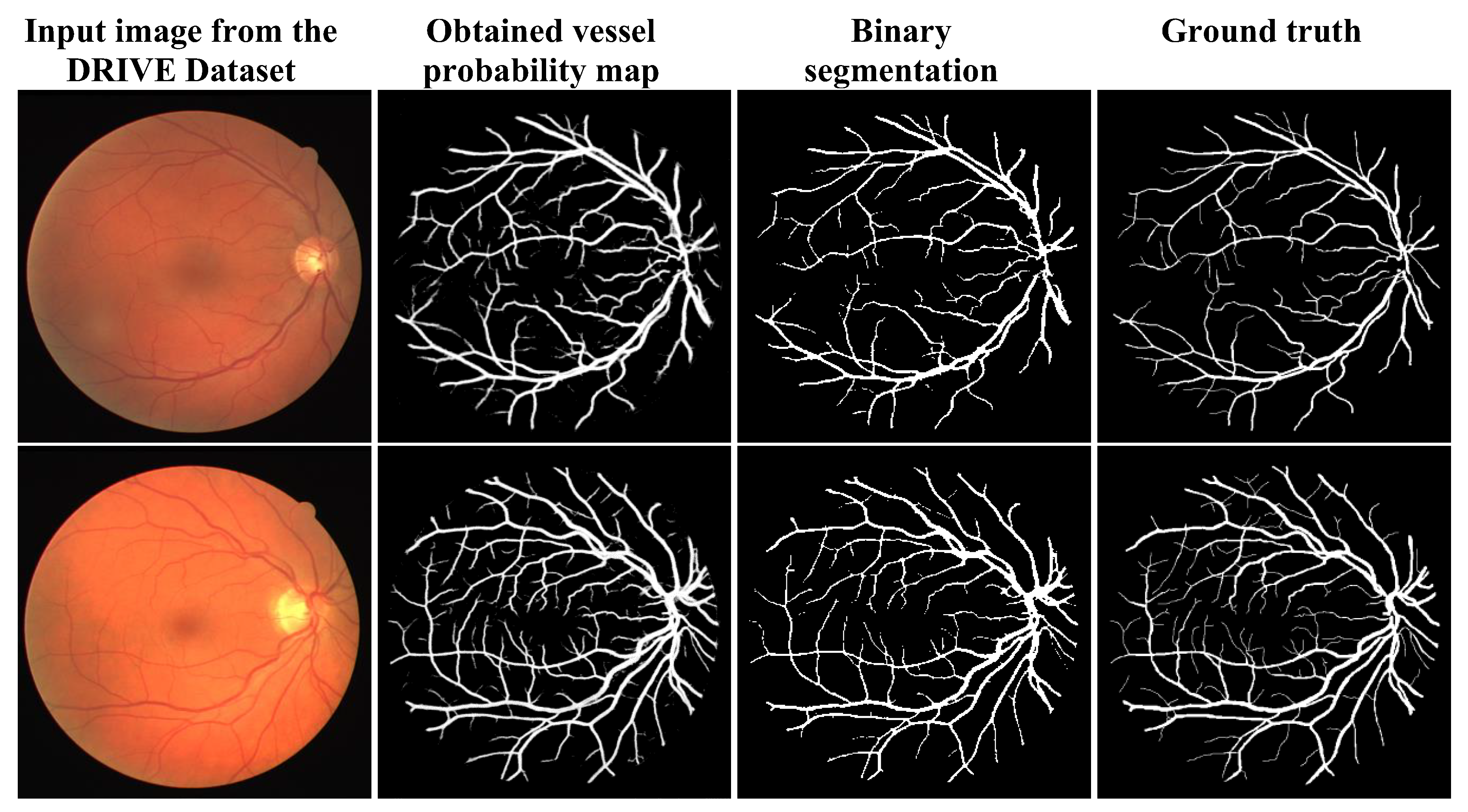
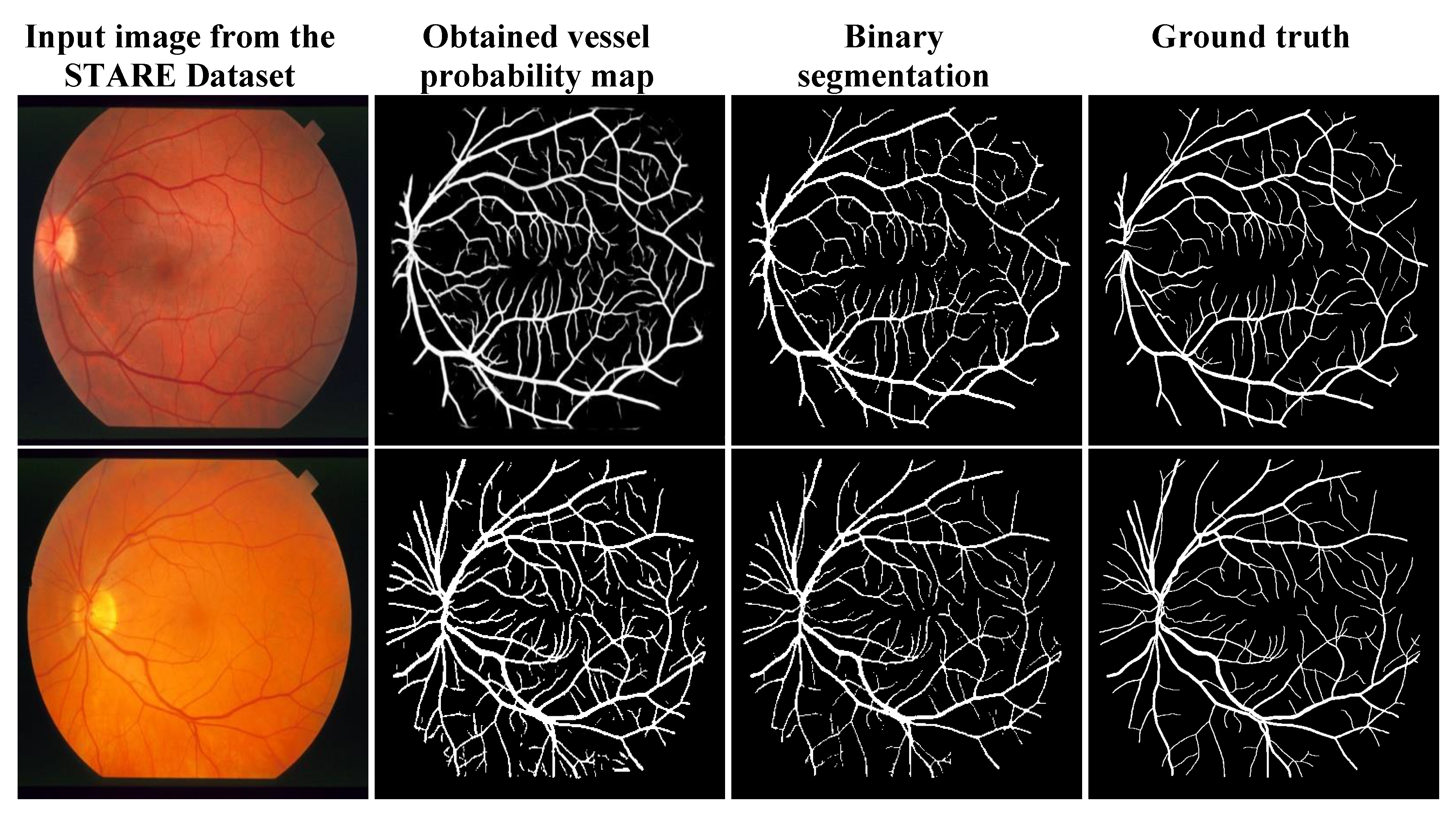
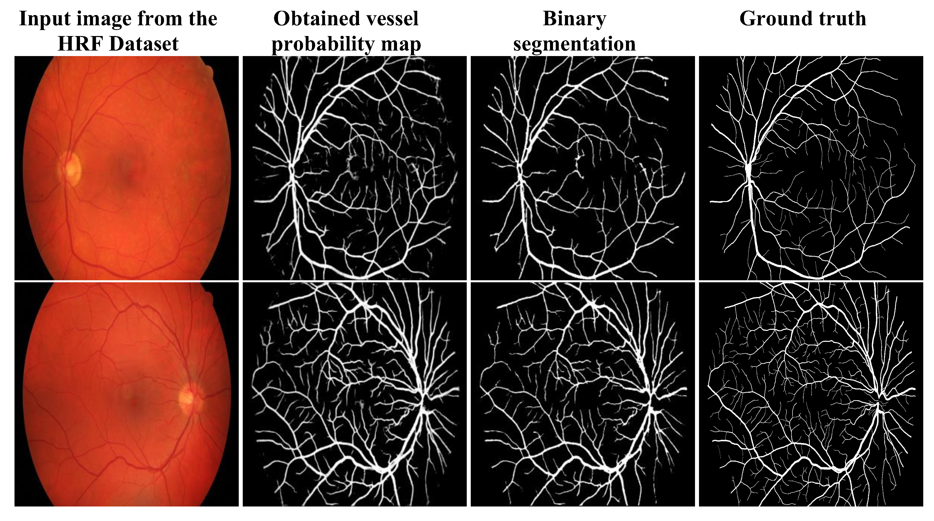
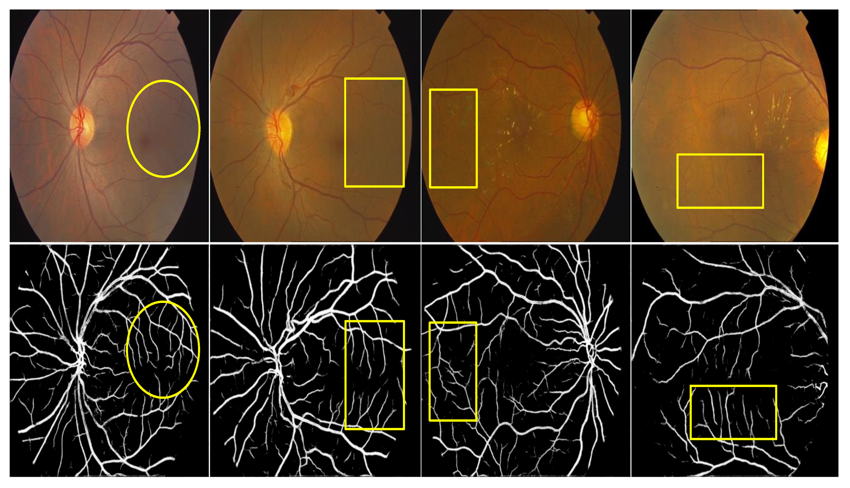
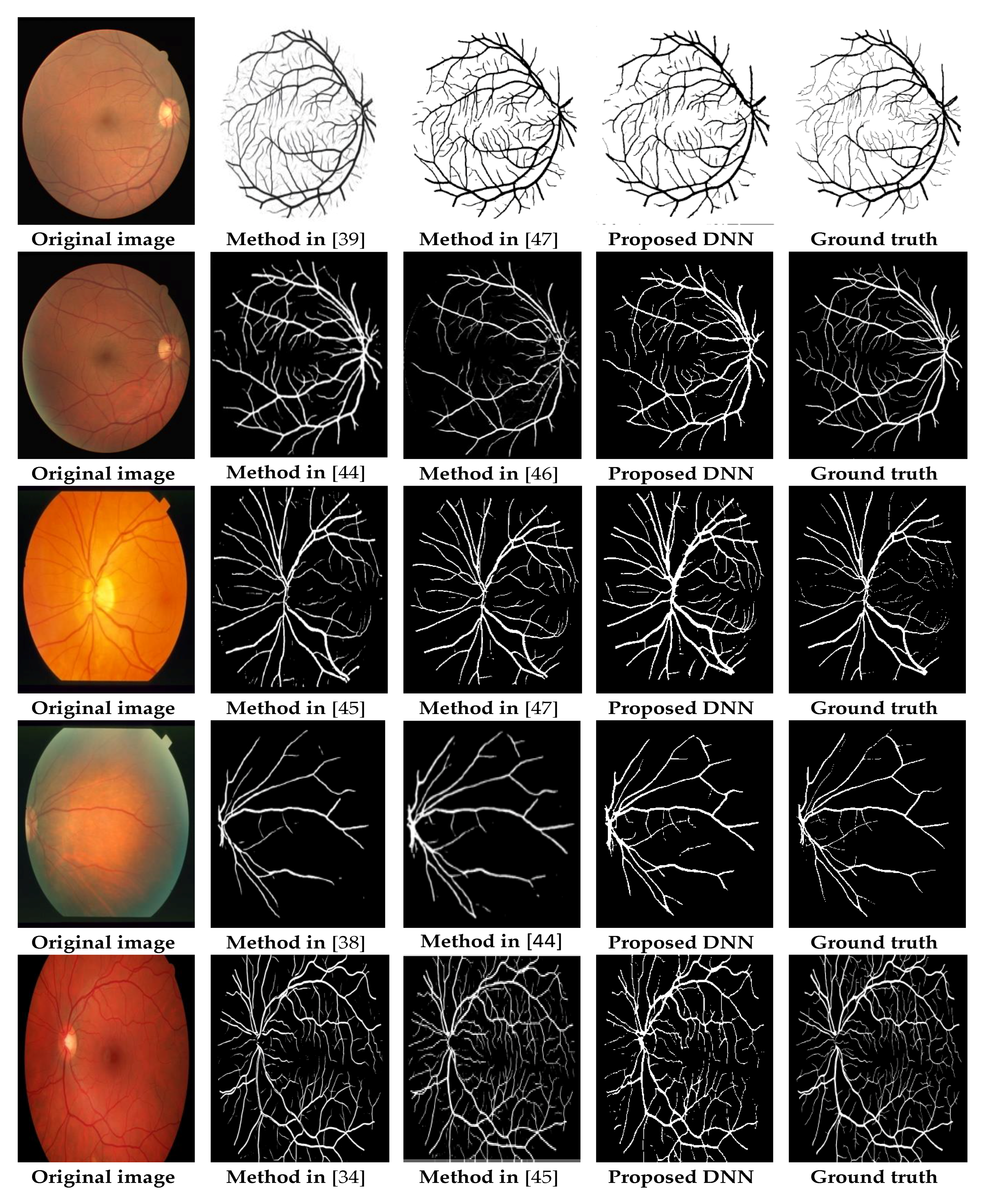
3.3. Qualitative Analysis

To assess the blood vessel segmented images qualitatively, the results of the proposed multilevel/multiscale DNN is compared with other popular supervised learning approaches. It is shown in Figure 11 along with the original image and the ground truth images.
In Figure 11, the first two row results are taken from DRIVE, the next two rows from STARE and the last row from HRF respectively. From Figure 11, the results obtained by Liskowski and Krawiec [39] segment the blood vessels more similarly to the ground truth but include a lot of background structures. Three stage segmenter [47] performs well in segmenting the thin vessels as shown in Figure 11. Multilevel FCN [44] uses information from multiple levels but still misses out the thin vessels during segmentation. Even though ground truth information was not used while training, this method was able to segment the vessels [46]. Eventually, it misses out a lot of vessels and it is tested only on DRIVE dataset. Dense conditional random forest (CRF) model which uses CNN as a feature extractor [45] segments the blood vessels but the segmentation contains disjoint vessel sections. A cross-modality autoencoder is unable to segment blood vessels that are present in the cluttered background [38]. Segmentation of blood vessels by the fully connected CRF [34] is inefficient to clearly segment the blood vessel structures compared to the deep learning approaches. The proposed multilevel/multiscale DNN segments most of the blood vessel sections efficiently but misses some of the thin vessels as shown in Figure 11. The highlighted blood vessels using the proposed preprocessing greatly aids in segmenting the vessels present in the cluttered background or ambiguous regions.

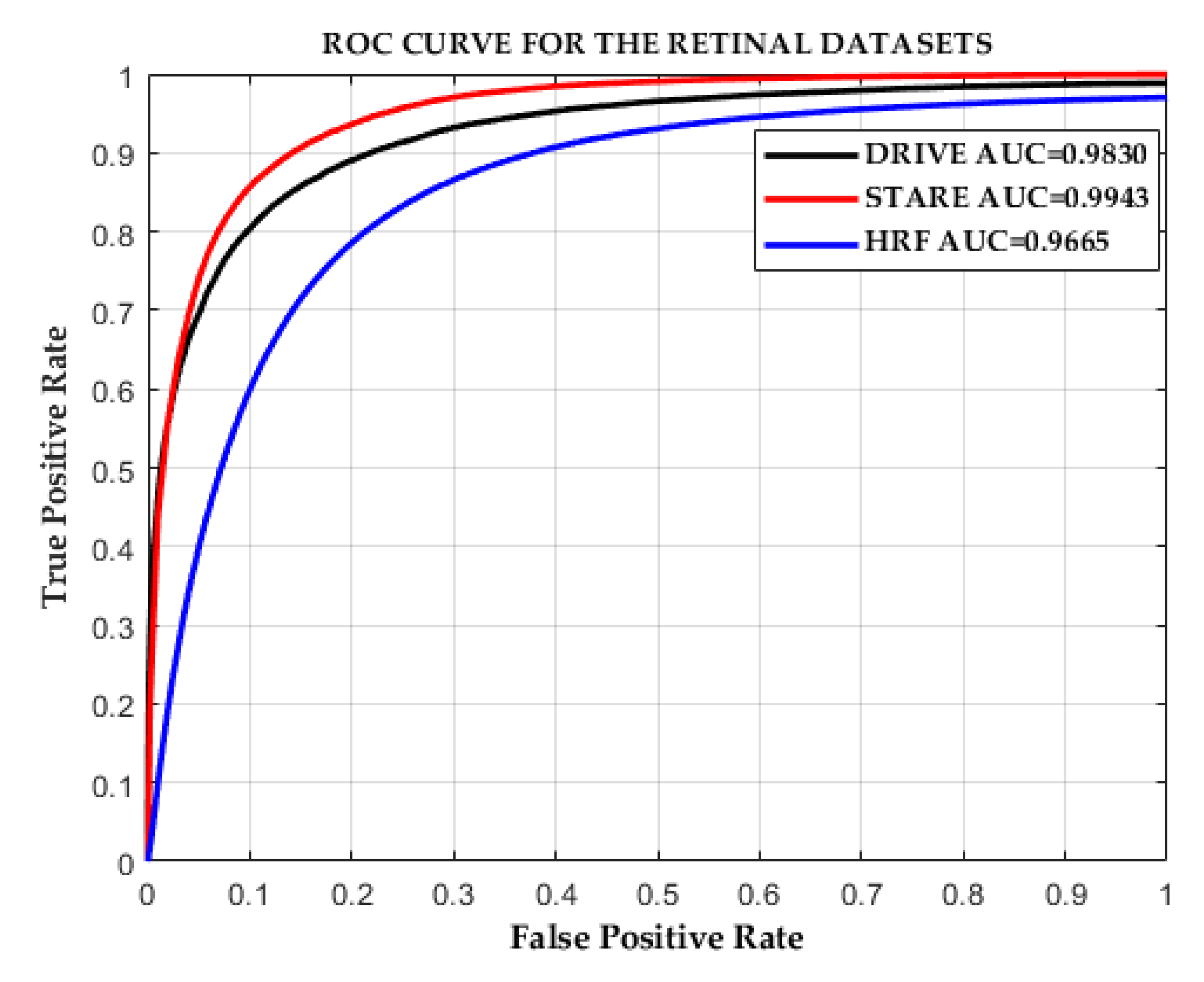
3.4. Quantitative Analysis

The performance metrics are compared against the prominent existing methods and with the recent deep learning methods. It is tabulated in Table 3.
Matched filtering approaches using Gaussian kernels have very low accuracy and AUC values. Matched filter kernels respond to both the vessel and non-vessel structures thereby reducing their performance [17,18]. Although multiscale approaches selectively use multiple scales to extract all the useful vessel information, they could not improve the accuracy in vessel segmentation [22,23]. Region growing method has improved AUC values such as 0.967 for both DRIVE and STARE because of the novel stopping criteria [26]. However, this method could reach a maximum accuracy of 0.949 in DRIVE and 0.956 in STARE respectively. Active contour models fit the curves to the vessel boundaries but it is a complex task to deform the curve structures. These methods have very low SN, SP, Acc and AUC values and their performance metrics are given in Table 3. Unsupervised technique segments the vessels by recognizing the vessel patterns iteratively but it gives poor segmentation results. The maximum accuracy obtained is only 0.9342 [31]. Supervised methods were able to perform well since they use a set of supervised features to learn the neural network model. It attains a maximum accuracy of 0.9513 and 0.9605 in DRIVE and STARE, respectively [35]. The increase in values of AUC shows improved blood vessel segmentation. Their AUC values are 0.9682 and 0.9789 for DRIVE and STARE datasets, respectively. Multiple scales and orientation features from the wavelet transform along with random forest classifier has improved performance metrics and achieves better AUC values [36].
Deep learning approaches perform well in vessel segmentation and also they do not need any artificially handcrafted features to train the neural networks. These approaches attain the highest SN, SP, Acc, and AUC values in both DRIVE and STARE datasets. While training the deep neural network, the retinal fundus images are given to the network as augmented small patches or the complete image itself. Training using the fundus patches degrades the training and testing efficiency, but the performance is quite good, as seen in Table 3 [38,39,45,47]. The observed performance metrics are higher for STARE in comparison to that in DRIVE. The five-stage neural network based autoencoder segments the blood vessels with high SP, Acc and AUC values for both DRIVE and STARE datasets [38]. The Liskowski et al. method reduces small vessel misclassification and provides an AUC value of 0.9880 in STARE [39]. It also has better SP and Acc values. Learned unary features given to the CRF for vessel segmentation gives a little lower accuracy value such as 0.9469 in DRIVE and 0.9585 in STARE [45]. The fusion of separately segmented thin and thick blood vessel approach gives better AUC, Acc and SP values, as given in Table 3 [47].
Using FCN, the training and testing become efficient but the performance metrics tend to decrease [42,43,44]. FCN combined with fully connected CRF gave less satisfying Acc and Sensitivity values for both the retinal datasets [42]. The results of Maninis et al. are reproduced by thresholding the probability maps with optimal threshold into binary segmentation [43]. Moreover, their quantitative performance metrics are found out and included in Table 3. Their approach achieves the highest AUC value in comparison to all the aforementioned references. This is because they used the training images from DRIVE to train the model and test the images from DRIVE using given test images obtained from a similar imaging source. Moreover, the width of the vessels after segmentation is larger than the ground truth which overshoots the SN values to greater values which are not acceptable. Multilevel deep supervision network segments the blood vessels with higher accuracy and SP values but its SN values are very low [44]. Also, the AUC values reach 0.9885 in STARE and 0.9782 in the DRIVE dataset, respectively. Though Chen did not use the ground truth for training the CNN, it could achieve slightly better SN, SP, Acc and AUC values as given in Table 3 [46].
The proposed multilevel/multiscale DNN, which also uses FCN, gave increased performance metrics as tabulated in Table 3. Deep supervision layers DS_1 and DS_2 that use Gaussian kernels extract blood vessel features from multiple layers at different scales. Moreover, the increase in the receptive field of these deep supervision layers makes the proposed DNN segment the blood vessels from almost any retinal fundus image with utmost precision. The proposed preprocessing that highlights the blood vessels is an added advantage during training. Therefore, the proposed DNN model achieves an accuracy of 0.9609 on DRIVE and 0.9646 on STARE. It is true that higher sensitivity denotes a higher true positive rate. The obtained SN values are 0.8282 and 0.8979 for DRIVE and STARE respectively. This method achieves better sensitivity in comparison to the existing classical segmentation methods and reaches an acceptable specificity value. The SP values are 0.9738 and 0.9701 in DRIVE and STARE datasets respectively. Also, the computed average AUC measures for the proposed DNN are higher for the STARE dataset in comparison to the DRIVE and HRF datasets. Though the AUC values for the test images in all the dataset gives better AUC values, STARE attains the highest value because the test images in STARE are easily segmented into both thin and thick vessels appropriately. But the thin vessels in DRIVE and HRF are hard to segment similar to the vessel ground truth dataset. Also, STARE contains only 10 test images and hence the average AUC value is higher for STARE in comparison to DRIVE and HRF.
Figure 12 depicts the ROC curves for the maximum AUC values obtained from DRIVE, STARE and HRF dataset for the proposed multilevel/multiscale DNN model.
The results of the proposed DNN model is improved in comparison to the existing methods with minimal iterations, minimal augmented input dataset and with minimal vessel-specific DS layers.

4. Discussion

Multilevel deep supervision layer DS_1 learns a lot of blood vessel features from all four stages in the proposed DNN. The learned blood vessel features include a lot of non-vessel regions and it is unable to localize the blood vessel regions appropriately. It is shown in Figure 13. But with multilevel/multiscale layers, i.e., both DS_1 and DS_2, the blood vessel regions are well localized excluding the non-vessel regions, presence of boundary and optic disc. The selection of multiple scales helps the network to learn the blood vessel regions alone leaving all the non-vessel regions. Hence, from Figure 13, it is clear that multilevel/multiscale DS_1 and DS_2 layer is able to learn blood vessel regions better when compared to multilevel DS_1 layer.
Using a single Gaussian convolution layer on top of the DS combinations will have a small receptive field. This could not improve the vessel segmentation. Hence, in this paper, the proposed model uses two convolution layers i.e., conv1_DS_8/16 and conv2_DS_8/16 layers on top of the multilevel/multistage DS combination. This widens the receptive field of the multilevel/multistage DS layers. This leads to localized and improved retinal blood vessel segmentation. Table 4 lists the performance metrics of proposed multilevel/multiscale DNN with the increase in receptive field for the images preprocessed using the mean value subtraction and the proposed preprocessing in DRIVE. The measured performance metrics are better with the addition of conv1_DS_8/16 and conv2_DS_8/16 when compared to the single conv1_DS_8/16 for the proposed preprocessing. For the images preprocessed with the proposed preprocessing, the addition of conv2_DS_8/16 partitions the blood vessels excluding the vessel neighbors and thus reduces the sensitivity values to 0.8282 from 0.8428. Its Acc and SP values are also higher. By contrast, for the mean value subtracted images the addition of conv2_DS_8/16 could not benefit since the segmented blood vessels are very thick with extreme SN values, as it includes neighboring pixels of the vessel structures.
Similarly, performance evaluation of the proposed DNN is done on the STARE after increasing the receptive field size. It is given in Table 5.
The proposed DNN model trained with the proposed preprocessed images that are tested in STARE dataset gave visibly better SN, SP and Acc values of 0.8979, 0.9701 and 0.9645, respectively. It has a much-improved performance measure with more localized blood vessel segmentation. On the other hand, testing the trained model with mean value subtracted images in STARE dataset gave very less satisfactory results. Addition of conv2_DS_8/16 fails to learn vessel features (outputs a void image for certain input) for the mean value subtracted images which lower the SN values. Since SN and SP are inversely proportional, SP values tend to overshoot. It is found that a further increase in the receptive field of view degrades the performance measure.
Finally, the resulting vessel probability map at the 18,000th iteration for only the multilevel/multiscale combination and together with its increased receptive field of view is discussed. It is depicted in Figure 14 for both the images preprocessed using mean value subtraction as well as with the proposed preprocessing.
Both Figure 14a,b contain an optic disc but the images segmented using the proposed preprocessing are clear at the macula rather than cluttered. Although Figure 14c trained using the mean value, subtracted input segments more blood vessels; there is no clear distinction between vessels and non-vessels. Non-vessel structures such as the optic disc, boundary, macula and uncertain regions are still present as marked in Figure 14c. However, the proposed model preprocessed using the proposed preprocessing, i.e., Figure 14d, shows improved accuracy in vessel segmentation without the presence of non-vessel regions as marked. It starts to localize the blood vessel regions precisely because of the receptive field size increase. In addition, it aids in obtaining error-free probability maps. It is well proven in Figure 14 that the increase in the receptive field of both the DS_1 and DS_2 layers helps the DNN to learn plenty of vessel features and localize them. The obtained blood vessel probability map closely resembles the ground truth image. But the segmented blood vessels after binary segmentation leave out the tiny blood vessels. Hence, research is being done to incorporate the postprocessing method to retain the tiny blood vessels from the probability map.
After the blood vessels are carefully segmented from the retinal fundus image, useful parameters can be computed from these vessel structures to diagnose DR, neovascularization, hypertension, stroke, cerebrovascular and cardiovascular disorders. The parameters include measuring vessel width, length, boundary, vessel curvature, vessel tortuosity, arteriolar–venular ratios, etc. Also, the removal of blood vessel structures aids in the segmentation of optic disc and cup for glaucoma diagnosis. The proposed multilevel/multiscale DNN can be extended to perform various vessel parameter computations for efficient vessel disorder diagnosis.
This automation of blood vessel diagnosis serves as an informative and quick aid for blood vessel analysis to an ophthalmologist. Automation cannot replace the ophthalmologist but it can speed up the process of diagnosis and aid in accurate quantitative measurements.

5. Conclusions

The segmentation task was laborious and less robust when the accuracy of vessel segmentation depended greatly on the expertise of man-made features. In this paper, a three-plane preprocessing technique is used to highlight the blood vessels before training the DNN. The proposed multilevel/multiscale DNN segments the retinal blood vessels without the use of input-supervised blood vessel features. This network is capable of learning vessel features at multiple scales and levels. The resulting segmented images obtained after training the model on the augmented dataset are tested on DRIVE, STARE, HRF, and real-world datasets. Qualitative analysis of the proposed DNN with other deep learning models is performed and the corresponding vessel segmentations are validated. Quantitative performance metrics are analyzed and it is found that the proposed model has better sensitivity and acceptable specificity and accuracy values in comparison with the remaining conventional segmentation approaches. Moreover, the AUC values are computed to justify the proper segmentation of blood vessel sections from the retina. The average AUC values obtained are 0.9786, 0.9892, and 0.9450 for DRIVE, STARE, and HRF datasets respectively. The segmented blood vessels are free from pathologies, optic disc, and ambiguous regions in the background. Still, the inclusion of better postprocessing approach is needed. In the future, these segmented retinal vessel profile can be extended for measuring vascular width, tortuosity, length, thickness, diameter, curvature, and arteriolar-venular ratios. The blood vessel types can also be classified to treat vessel disorders. It has also been identified that the changes in the retinal vessels not only identify DR, hypertension, and stroke but also related cardiovascular and cerebrovascular diseases.

Author Contributions

Conceptualization, P.M.S. and T.V.; methodology, P.M.S.; software, P.M.S.; validation, P.M.S., T.V.; formal analysis, T.V.; investigation, T.V.; resources, T.V.; data curation, P.M.S.; writing—original draft preparation, P.M.S.; writing—review and editing, T.V.; visualization, P.M.S.; supervision, T.V.; project administration, T.V.; funding acquisition, P.M.S.

Funding

This research was funded by the Council of Scientific And Industrial Research, India, grant number 09/844(0040)/2016 EMR-I.

Acknowledgments

The authors would like to acknowledge M. Arun for providing the GPU to carry out this research work. The authors are grateful for the generous support of Mulamoottil Eye Hospital, Kerala, India for providing the real-world retinal images.

Conflicts of Interest

The authors declare no conflict of interest.

References

  1. Taylor, H.R.; Keeffe, J.E. World blindness: A 21st century perspective. Br. J. Ophthalmol. 2001, 85, 261–266. [Google Scholar] [CrossRef] [PubMed]
  2. Mateen, M.; Wen, J.; Nasrullah; Song, S.; Huang, Z. Fundus image classification using VGG-19 architecture with PCA and SVD. Symmetry 2019, 11, 1. [Google Scholar] [CrossRef]
  3. Popescu, D.; Ichim, L. Intelligent image processing system for detection and segmentation of regions of interest in retinal images. Symmetry 2018, 10, 73. [Google Scholar] [CrossRef]
  4. Han, H.C. Twisted blood vessels: Symptoms, etiology and biomechanical mechanisms. J. Vasc. Res. 2012, 49, 185–197. [Google Scholar] [CrossRef] [PubMed]
  5. Moss, H.E. Retinal vascular changes are a marker for cerebral vascular diseases. Curr. Neurol. Neurosci. Rep. 2015, 15, 40. [Google Scholar] [CrossRef] [PubMed]
  6. Hassan, S.S.A.; Bong, D.B.L.; Premsenthil, M. Detect on of neovascularization in diabetic retinopathy. J. Digit. Imaging 2012, 25, 437–444. [Google Scholar] [CrossRef] [PubMed]
  7. Wong, T.Y.; Klein, R.; Klein, B.E.K.; Tielsch, J.M.; Hubbard, L.; Nieto, F.J. Retinal microvascular abnormalities and their relationship with hypertension, cardiovascular disease, and mortality. Surv. Ophthalmol. 2001, 46, 59–80. [Google Scholar] [CrossRef]
  8. Nowilaty, S.; Al-Shamsi, H.; Al-Khars, W. Idiopathic juxtafoveolar retinal telangiectasis: A current review. Middle East Afr. J. Ophthalmol. 2010, 17, 224. [Google Scholar] [CrossRef]
  9. Niemeijer, M.; Xu, X.; Dumitrescu, A.V.; Gupta, P.; Van Ginneken, B.; Folk, J.C.; Abramoff, M.D. Automated measurement of the arteriolar-to-venular width ratio in digital color fundus photographs. IEEE Trans. Med. Imaging 2011, 30, 1941–1950. [Google Scholar] [CrossRef]
  10. Ünver, H.; Kökver, Y.; Duman, E.; Erdem, O. Statistical edge detection and circular hough transform for optic disk localization. Appl. Sci. 2019, 9, 350. [Google Scholar] [CrossRef]
  11. Al-Bander, B.; Williams, B.M.; Al-Nuaimy, W.; Al-Taee, M.A.; Pratt, H.; Zheng, Y. Dense fully convolutional segmentation of the optic disc and cup in colour fundus for glaucoma diagnosis. Symmetry 2018, 10, 87. [Google Scholar] [CrossRef]
  12. Sarathi, M.P.; Dutta, M.K.; Singh, A.; Travieso, C.M. Blood vessel inpainting based technique for efficient localization and segmentation of optic disc in digital fundus images. Biomed. Signal Process. Control 2016, 25, 108–117. [Google Scholar] [CrossRef]
  13. Almotiri, J.; Elleithy, K.; Elleithy, A. Retinal vessels Segmentation techniques and algorithms: A survey. Appl. Sci. 2018, 8, 155. [Google Scholar] [CrossRef]
  14. Yang, Y.; Huang, S.; Rao, N. An automatic hybrid method for retinal blood vessel extraction. Int. J. Appl. Math. Comput. Sci. 2008, 18, 399–407. [Google Scholar] [CrossRef]
  15. Chaudhuri, S.; Chatterjee, S.; Katz, N.; Nelson, M.; Goldbaum, M. Detection of blood vessels in retinal images using two-dimensional matched filters. IEEE Trans. Med. Imaging 1989, 8, 263–269. [Google Scholar] [CrossRef] [PubMed] [Green Version]
  16. Al-Rawi, M.; Qutaishat, M.; Arrar, M. An improved matched filter for blood vessel detection of digital retinal images. Comput. Biol. Med. 2007, 37, 262–267. [Google Scholar] [CrossRef] [PubMed]
  17. Chakraborti, T.; Jha, D.K.; Chowdhury, A.S.; Jiang, X. A self-adaptive matched filter for retinal blood vessel detection. Mach. Vis. Appl. 2014, 26, 55–68. [Google Scholar] [CrossRef]
  18. Singh, N.P.; Srivastava, R. Retinal blood vessels segmentation by using Gumbel probability distribution function based matched filter. Comput. Methods Programs Biomed. 2016, 129, 40–50. [Google Scholar] [CrossRef]
  19. Dharmawan, D.A.; Ng, B.P.; Rahardja, S. A modified Dolph-Chebyshev type II function matched filter for retinal vessels segmentation. Symmetry 2018, 10, 257. [Google Scholar] [CrossRef]
  20. Frangi, A.; Niessen, W.; Vincken, K.; Viergever, M. Multiscale vessel enhancement filtering medical image computing and computer-assisted interventation—MICCAI. In Medical Image Computing and Computer-Assisted Interventation—MICCAI’98; Springer: Berlin/Heidelberg, Germany, 1998; Volume 1496, pp. 130–137. ISBN 978-3-540-65136-9. [Google Scholar]
  21. Sofka, M.; Stewart, C.V. Retinal vessel centerline extraction using multiscale matched filters, confidence and edge measures. IEEE Trans. Med. Imaging 2006, 25, 1531–1546. [Google Scholar] [CrossRef]
  22. Saffarzadeh, V.M.; Osareh, A.; Shadgar, B. Vessel segmentation in retinal images using multi-scale line operator and K-means clustering. J. Med. Signals Sens. 2014, 4, 122–129. [Google Scholar] [PubMed]
  23. Zhang, L.; Fisher, M.; Wang, W. Retinal vessel segmentation using multi-scale textons derived from keypoints. Comput. Med. Imaging Graph. 2015, 45, 47–56. [Google Scholar] [CrossRef] [PubMed] [Green Version]
  24. Joshi, V.S.; Reinhardt, J.M.; Garvin, M.K.; Abramoff, M.D. Automated method for identification and artery-venous classification of vessel trees in retinal vessel networks. PLoS ONE 2014, 9, e88061. [Google Scholar] [CrossRef] [PubMed]
  25. Lázár, I.; Hajdu, A. Segmentation of retinal vessels by means of directional response vector similarity and region growing. Comput. Biol. Med. 2015, 66, 209–221. [Google Scholar] [CrossRef] [PubMed]
  26. Roychowdhury, S.; Koozekanani, D.D.; Parhi, K.K. Iterative Vessel segmentation of fundus images. IEEE Trans. Biomed. Eng. 2015, 62, 1738–1749. [Google Scholar] [CrossRef] [PubMed]
  27. Al-Diri, B.; Hunter, A.; Steel, D. An active contour model for segmenting and measuring retinal vessels. IEEE Trans. Med. Imaging 2009, 28, 1488–1497. [Google Scholar] [CrossRef] [PubMed]
  28. Zhao, Y.; Rada, L.; Chen, K.; Harding, S.P.; Zheng, Y. Automated Vessel segmentation using infinite perimeter active contour model with hybrid region Information with application to retinal images. IEEE Trans. Med. Imaging 2015, 34, 1797–1807. [Google Scholar] [CrossRef] [PubMed]
  29. Zhao, Y.; Zhao, J.; Yang, J.; Liu, Y.; Zhao, Y.; Zheng, Y.; Xia, L.; Wang, Y. Saliency driven vasculature segmentation with infinite perimeter active contour model. Neurocomputing 2017, 259, 201–209. [Google Scholar] [CrossRef] [Green Version]
  30. Kande, G.B.; Subbaiah, P.V.; Savithri, T.S. Unsupervised fuzzy based vessel segmentation in pathological digital fundus images. J. Med. Syst. 2010, 34, 849–858. [Google Scholar] [CrossRef]
  31. Allen, K.; Joshi, N.; Noble, J.A. Tramline and NP windows estimation for enhanced unsupervised retinal vessel segmentation. In Proceedings of the International Symposium on Biomedical Imaging, Chicago, IL, USA, 30 March–2 April 2011; pp. 1387–1390. [Google Scholar]
  32. Soares, J.V.B.; Leandro, J.J.G.; Cesar, R.M.; Jelinek, H.F.; Cree, M.J. Retinal vessel segmentation using the 2-D Gabor wavelet and supervised classification. IEEE Trans. Med. Imaging 2006, 25, 1214–1222. [Google Scholar] [CrossRef] [Green Version]
  33. Rahebi, J.; Hardalaç, F. Retinal blood vessel segmentation with neural network by using gray-level co-occurrence matrix-based features patient facing systems. J. Med. Syst. 2014, 38, 85. [Google Scholar] [CrossRef] [PubMed]
  34. Orlando, J.I.; Blaschko, M. Learning fully-connected CRFs for blood vessel segmentation in retinal images. In Proceedings of the International Conference on Medical Image Computing and Computer-Assisted Intervention, Boston, MA, USA, 14–18 September 2014. Lecture Notes in Computer Science (including Subseries Lecture Notes in Artificial Intelligence and Lecture Notes in Bioinformatics). [Google Scholar]
  35. Aslani, S.; Sarnel, H. A new supervised retinal vessel segmentation method based on robust hybrid features. Biomed. Signal Process. Control 2016, 30, 1–12. [Google Scholar] [CrossRef]
  36. Zhang, J.; Chen, Y.; Bekkers, E.; Wang, M.; Dashtbozorg, B.; ter Haar Romeny, B.M. Retinal vessel delineation using a brain-inspired wavelet transform and random forest. Pattern Recognit. 2017, 69, 107–123. [Google Scholar] [CrossRef]
  37. Guo, Y.; Budak, Ü.; Şengür, A.; Smarandache, F. A retinal Vessel detection approach based on Shearlet transform and indeterminacy filtering on fundus images. Symmetry 2017, 9, 235. [Google Scholar] [CrossRef]
  38. Li, Q.; Feng, B.; Xie, L.; Liang, P.; Zhang, H.; Wang, T. A cross-modality learning approach for vessel segmentation in retinal images. IEEE Trans. Med. Imaging 2016, 35, 109–118. [Google Scholar] [CrossRef] [PubMed]
  39. Liskowski, P.; Krawiec, K. Segmenting retinal blood vessels with deep neural networks. IEEE Trans. Med. Imaging 2016, 35, 2369–2380. [Google Scholar] [CrossRef] [PubMed]
  40. Wu, A.; Xu, Z.; Gao, M.; Buty, M.; Mollura, D.J. Deep vessel tracking: A generalized probabilistic approach via deep learning. In Proceedings of the International Symposium on Biomedical Imaging, Prague, Czech Republic, 13–16 April 2016; pp. 1363–1367. [Google Scholar]
  41. Xie, S.; Tu, Z. Holistically-Nested Edge Detection. Int. J. Comput. Vis. 2017, 1–16. [Google Scholar] [CrossRef]
  42. Fu, H.; Xu, Y.; Wong, D.W.K.; Liu, J. Retinal vessel segmentation via deep learning network and fully-connected conditional random fields. In Proceedings of the International Symposium on Biomedical Imaging, Prague, Czech Republic, 13–16 April 2016; pp. 698–701. [Google Scholar]
  43. Maninis, K.K.; Pont-Tuset, J.; Arbeláez, P.; Van Gool, L. Deep Retinal Image Understanding; Lecture Notes in Computer Science (including subseries Lecture Notes in Artificial Intelligence and Lecture Notes in Bioinformatics); Springer: Cham, Switzerland, 2016; Volume 9901 LNCS, pp. 140–148. [Google Scholar]
  44. Mo, J.; Zhang, L. Multi-level deep supervised networks for retinal vessel segmentation. Int. J. Comput. Assist. Radiol. Surg. 2017, 12, 2181–2193. [Google Scholar] [CrossRef] [PubMed]
  45. Zhou, L.; Yu, Q.; Xu, X.; Gu, Y.; Yang, J. Improving dense conditional random field for retinal vessel segmentation by discriminative feature learning and thin-vessel enhancement. Comput. Methods Programs Biomed. 2017, 148, 13–25. [Google Scholar] [CrossRef] [PubMed]
  46. Chen, Y. A Labeling-free approach to supervising deep neural networks for retinal blood Vessel segmentation. arXiv 2017, arXiv:1704.07502. [Google Scholar]
  47. Yan, Z.; Yang, X.; Cheng, K.T.T. A Three-stage deep learning model for accurate retinal Vessel segmentation. IEEE J. Biomed. Health Inform. 2019, 23, 1427–1436. [Google Scholar] [CrossRef] [PubMed]
  48. Niemeijer, M.; Staal, J.; van Ginneken, B.; Loog, M.; Abràmoff, M.D. Comparative study of retinal vessel segmentation methods on a new publicly available database. In Proceedings of the Medical Imaging 2004, Medical Imaging 2004: Image Processing, San Diego, CA, USA, 12 May 2004; Volume 5370, pp. 648–656. [Google Scholar]
  49. Hoover, A. Locating blood vessels in retinal images by piecewise threshold probing of a matched filter response. IEEE Trans. Med. Imaging 2000, 19, 203–210. [Google Scholar] [CrossRef] [PubMed]
  50. Odstrcilik, J.; Kolar, R.; Kubena, T.; Cernosek, P.; Budai, A.; Hornegger, J.; Gazarek, J.; Svoboda, O.; Jan, J.; Angelopoulou, E. Retinal vessel segmentation by improved matched filtering: Evaluation on a new high-resolution fundus image database. IET Image Process. 2013, 7, 373–383. [Google Scholar] [CrossRef]
  51. Zuiderveld, K. Contrast Limited Adaptive Histogram Equalization. In Graphics Gems; Academic Press Professional, Inc.: San Diego, CA, USA, 1994; pp. 474–485. ISBN 0-12-336155-9. [Google Scholar]
  52. Simonyan, K.; Zisserman, A. Very Deep Convolutional Networks for Large-Scale Image Recognition. In Proceedings of the 3rd International Conference on Learning Representations, San Diego, CA, USA, 7–9 May 2015. [Google Scholar]
  53. Zhang, Y.D.; Dong, Z.; Chen, X.; Jia, W.; Du, S.; Muhammad, K.; Wang, S.H. Image based fruit category classification by 13-layer deep convolutional neural network and data augmentation. Multimed. Tools Appl. 2019, 78, 3613–3632. [Google Scholar] [CrossRef]
  54. Wang, S.; Sun, J.; Mehmood, I.; Pan, C.; Chen, Y.; Zhang, Y.D. Cerebral micro-bleeding identification based on a nine-layer convolutional neural network with stochastic pooling. Concurr. Comput. 2019, e5130. [Google Scholar] [CrossRef]
  55. Jia, Y.; Shelhamer, E.; Donahue, J.; Karayev, S.; Long, J.; Girshick, R.; Guadarrama, S.; Darrell, T. Caffe: Convolutional architecture for fast feature embedding. In Proceedings of the 22nd ACM International Conference on Multimedia (ACM 2014), Orlando, FL, USA, 3–7 November 2014; pp. 675–678. [Google Scholar]
Figure 1. Pre-processed images obtained from retinal datasets.
Symmetry 11 00946 g001
Figure 2. Proposed deep neural network (DNN) model for retinal blood vessel segmentation.
Symmetry 11 00946 g002
Figure 3. (a) Cross section of vessel highlighted, (b) Gaussian profile of the cross section.
Symmetry 11 00946 g003
Figure 4. The argument of maxima of output activations for the eight vessel-specific feature maps from the four convolution layers.
Symmetry 11 00946 g004
Figure 5. The argument of maxima of output activations for the 16 vessel-specific feature maps from the four convolution layers.
Symmetry 11 00946 g005
Figure 6. A pictorial view of the increase in receptive field size with 3 × 3 filters and no padding on a 9 × 9 input.
Symmetry 11 00946 g006
Figure 7. Blood vessel segmentation results obtained using the proposed DNN model in the Digital Retinal Images for Vessel Extraction (DRIVE) dataset.
Symmetry 11 00946 g007
Figure 8. Blood vessel segmentation results obtained using the proposed DNN model in the STructured Analysis of the Retina (STARE) dataset.
Symmetry 11 00946 g008
Figure 9. Blood vessel segmentation results obtained using the proposed DNN model in the High-Resolution Fundus (HRF) dataset.
Symmetry 11 00946 g009
Figure 10. First row depicts the real-world retinal images and the second row shows the corresponding blood vessel probability maps obtained using the proposed DNN model.
Symmetry 11 00946 g010
Figure 11. Qualitative analysis of the blood vessel segmented results in DRIVE, STARE and HRF datasets.
Symmetry 11 00946 g011
Figure 12. Plot of receiver operating characteristic (ROC) for the retinal DRIVE, STARE and HRF datasets.
Symmetry 11 00946 g012
Figure 13. Vessel segmentation using (a) DS_1 layer, (b) DS_1 and DS_2 layers. (c) Ground truth.
Symmetry 11 00946 g013
Figure 14. (ad) Vessel probability map for mean value subtracted images and the proposed preprocessed input images before and after the increase in the receptive field at the 18,000th iteration, (e) ground truth image.
Symmetry 11 00946 g014
Table 1. Formation of deep supervision (DS) layers.
Formation of DS_1 LayerSize [Width, Height, Depth]Formation of DS_2 LayerSize [Width, Height, Depth]
[ C o n v 1 _ 2 ] 8 [ C o n v 2 _ 2 ] 8 & [ D e C o n v 2 _ 2 ] 8 [ C o n v 3 _ 3 ] 8 & [ D e C o n v 3 _ 3 ] 8 [ C o n v 4 _ 3 ] 8 & [ D e C o n v 4 _ 3 ] 8 [ 562 562 8 ] [ 564 564 8 ] [ 568 568 8 ] [ 576 576 8 ] [ C o n v 1 _ 2 ] 16 [ C o n v 2 _ 2 ] 16 & [ D e C o n v 2 _ 2 ] 16 [ C o n v 3 _ 3 ] 16 & [ D e C o n v 3 _ 3 ] 16 [ C o n v 4 _ 3 ] 16 & [ D e C o n v 4 _ 3 ] 16 [ 562 562 16 ] [ 564 564 16 ] [ 568 568 16 ] [ 576 576 16 ]
Crop [ 562 562 8 ] [ 562 562 8 ] [ 562 562 8 ] [ 562 562 8 ] Crop [ 562 562 16 ] [ 562 562 16 ] [ 562 562 16 ] [ 562 562 16 ]
Concatenate (DS_1) [ 562 562 32 ] Concatenate (DS_2) [ 562 562 64 ]
Table 2. Layers in the proposed DNN with their respective sizes, number of activation maps and weights.
Layers in the Proposed DNNOutput Size [Width, Height, Depth]Activation MapsParameters (Weights)
Input image[562 562 3]3 planes
Conv 1_1[562 562 64]64(3 × 3 × 3 + 1) × 64 = 1792
Conv 1_2[562 562 64]64(3 × 3 × 64 + 1) × 64 = 36,928
Max pooling[281 281 64]640
Conv 2_1[281 281 128]128(3 × 3 × 64 + 1) × 128 = 73,856
Conv 2_2[281 281 128]128(3 × 3 × 128 + 1) × 128 = 147,584
Max pooling[141 141 128]1280
Conv 3_1[141 141 256]256(3 × 3 × 128 + 1) × 256 = 295,168
Conv 3_2[141 141 256]256(3 × 3 × 256 + 1) × 256 = 590,080
Conv 3_3[141 141 256]256(3 × 3 × 256 + 1) × 256 = 590,080
Max pooling[71 71 256]2560
Conv 4_1[71 71 512]512(3 × 3 × 256 + 1) × 512 = 1,180,160
Conv 4_2[71 71 512]512(3 × 3 × 512 + 1) × 512 = 2,359,808
Conv 4_3[71 71 512]512(3 × 3 × 512 + 1) × 512 = 2,359,808
DS_1 layer[562 562 32](8 × 4 = 32)[(3 × 3 × 64 + 1) × 8 + (3 × 3 × 128 + 1) × 8 +
(3 × 3 × 256 + 1) × 8 + (3 × 3 × 512 + 1) × 8] = 69,152
DS_2 layer[562 562 64](16 × 4 = 64)[(3 × 3 × 64 + 1) × 16 + (3 × 3 × 128 + 1) × 16 +
(3 × 3 × 256 + 1) × 16 + (3 × 3 × 512 + 1) × 16] = 138,304
Conv1_DS_8/16 layer[562 562 32/64]32/64(3 × 3 × 32 + 1) × 32 = 9248/3 × 3× 32 + 1) × 64 = 18,496
Conv2_DS_8/16 layer[562 562 32/64]32/64(3 × 3 × 32 + 1) × 32 = 9248/3 × 3 × 32 + 1) × 64 = 18,496
sp1/sp2[562 562 1/1]1/1(1 × 1 × 32 + 1) × 1 = 33/(1 × 1 × 64 + 1) × 1 = 65
Final 1 × 1 conv output[562 562 1]1(1 × 1 × 2 + 1) × 1 = 3
Table 3. Comparison of performance metrics for various methods in DRIVE and STARE.
MethodAuthor/Year/Ref.Metrics Obtained from DRIVE DatasetMetrics Obtained from STARE Dataset
SNSPAccAUCSNSPAccAUC
Ophthalmologist0.77630.97230.947-0.89510.93840.9348-
Matched filterChakraborti et al. (2014) [17]0.72050.95790.93700.94190.67860.95860.9379-
Singh, Srivatsava (2016) [18]0.75940.97080.95220.92870.79390.93760.92700.9140
Multi-scale approachSaffarzadeh et al. (2014) [22]--0.93870.9303--0.94830.9431
Zhang, Fisher, et al. (2015) [23]0.78120.96680.9504-----
Region growing methodLazar and Hajdu (2015) [25]0.76460.97230.9458-0.72480.97510.9492-
Roychowdhury et al. (2015) [26]0.7390.9780.9490.9670.7320.9840.9560.967
Active contour modelZhao, Rada, et al. (2015) [28]0.7420.9820.9540.8620.7800.9780.9560.874
Zhao, Zhao, et al. (2017) [29]0.7820.9790.9570.8860.7890.9780.9560.885
Unsupervised methodKande et al. (2010) [30]--0.89110.9518--0.89760.9298
Allen et al. (2011) [31]--0.9342 ----
Supervised methodAslani and Sarnel (2016) [35]0.75450.98010.95130.96820.75560.98370.96050.9789
Zhang, Chen, et al. (2017) [36]0.78610.97120.94660.97030.78820.97290.95470.9740
Deep learning methodLi et al. (2016) [38]0.75690.98160.95270.97380.77260.98440.96280.9879
Liskowski and Krawiec (2016) [39]0.75200.98060.95150.97100.81450.98660.96960.9880
Fu et al. (2016) [42]0.7294-0.947-0.714-0.9545-
Maninis et al. (2016) [43]0.94970.93770.93860.9862 0.94030.95520.95430.9748
Mo and Zhang (2017) [44]0.77790.97800.95210.97820.81470.98440.96740.9885
Zhou et al. (2017) [45]0.80780.96740.9469-0.80650.97610.9585-
Chen (2017) [46]0.74260.97350.94530.95160.72950.96960.94490.9557
Yan et al. (2018) [47]0.76310.98200.95380.97500.77350.98570.96380.9833
Proposed method 0.82820.97380.96090.97860.89790.97010.96460.9892
Table 4. Performance evaluation after increasing the receptive field in the DRIVE dataset.
DNN FrameworkPreprocessed with Mean Value SubtractionPreprocessed with the Proposed Preprocessing
SNSPAccSNSPAcc
Front end: 4 stages of VGG-16
Fine-tuning phase: DS_1 and DS_2 layers with a conv1_DS_8/16 layer
0.84740.96520.95470.84280.96770.9560
Front end: 4 stages of VGG-16
Fine-tuning phase: DS_1 and DS_2 layers with conv1_DS_8/16 & conv2_DS_8/16 layers (our model)
0.90580.95140.94720.82820.97380.9609
Table 5. Performance evaluation after increasing the receptive field in STARE dataset.
DNN FrameworkPreprocessed with Mean Value SubtractionPreprocessed with the Proposed Preprocessing
SNSPAccSNSPAcc
Front end: 4 stages of VGG-16
Fine-tuning phase: DS_1 and DS_2 layers with a conv1_DS_ 8/16 layer
0.65810.95810.93790.91990.96300.9599
Front end: 4 stages of VGG-16
Fine-tuning phase: DS_1 and DS_2 layers with conv1_DS_8/16 and conv2_DS_8/16 layers (our model)
0.41840.98750.94610.89790.97010.9645

