Article

Study on a Novel Fault Diagnosis Method Based on VMD and BLM

1
Software Institute, Dalian Jiaotong University, Dalian 116028, China
2
The State Key Laboratory of Mechanical Transmissions, Chongqing University, Chongqing 400044, China
3
Traction Power State Key Laboratory of Southwest Jiaotong University, Chengdu 610031, China
4
College of Marine Electrical Engineering, Dalian Maritime University, Dalian 116026, China
*
Author to whom correspondence should be addressed.
Symmetry 2019, 11(6), 747; https://doi.org/10.3390/sym11060747
Submission received: 24 April 2019 / Revised: 22 May 2019 / Accepted: 30 May 2019 / Published: 2 June 2019
(This article belongs to the Special Issue Symmetry in Engineering Sciences)

Abstract

:
The bearing system of an alternating current (AC) motor is a nonlinear dynamics system. The working state of rolling bearings directly determines whether the machine is in reliable operation. Therefore, it is very meaningful to study the fault diagnosis and prediction of rolling bearings. In this paper, a new fault diagnosis method based on variational mode decomposition (VMD), Hilbert transform (HT), and broad learning model (BLM), called VHBLFD is proposed for rolling bearings. In the VHBLFD method, the VMD is used to decompose the vibration signals to obtain intrinsic mode functions (IMFs). The HT is used to process the IMFs to obtain Hilbert envelope spectra, which are transformed into the mapped features and the enhancement nodes of BLM according to the complexity of the modeling tasks, and the nonlinear transformation mean according to the characteristics of input data. The BLM is used to classify faults of the rolling bearings of the AC motor. Next, the pseudo-inverse operation is used to obtain the fault diagnosis results. Finally, the VHBLFD is validated by actual vibration data. The experiment results show that the BLM can quickly and accurately be trained. The VHBLFD method can achieve higher identification accuracy for multi-states of rolling bearings and takes on fast operation speed and strong generalization ability.

1. Introduction

The working state of rolling bearings directly determines the reliable operation of a machine [1,2]. However, the occurrence probability of fault is always higher due to the influences of the load of rolling bearings of AC motor [3,4,5,6]. Thus, it is very important to improve the operation reliability and accurately diagnose faults for rolling bearings in time [7,8,9].
Fault diagnosis methods of rolling bearings are used to essentially recognize the working states [10,11,12,13]. To effectively recognize the working state of rolling bearings, many signal processing methods have been proposed in recent years, such as short time Fourier transform (STFT) [14,15], wavelet transform (WT) [16], Hilbert–Huang transform (HHT) [17,18,19], empirical mode decomposition (EMD) [20,21,22], entropy [23,24,25], support vector machine (SVM) [26], artificial intelligence methods [27,28,29], and other processing methods [30,31]. In addition, some new methods have also been applied in the field of signal analysis and fault diagnosis [32,33]. Gao et al. [34] proposed a fault identification method based on time-frequency distribution (TFD) for rolling bearings. Zhang et al. [35] proposed a flexible wavelet transform to obtain weak fault feature. Kabla et al. [36] applied HHT and marginal spectrum to analyze the signals of the stator current. Yuan et al. [37] proposed an ensemble noise-reconstructed EMD method. The SVM is widely applied for fault diagnosis. Du et al. [38] proposed a stochastic fault diagnosis method using EMD and principal component analysis (PCA). To solve the classification ability of SVM, Fei et al. [39] proposed a power transformer fault diagnosis model using a rough set and SVM. Gao et al. [40] proposed a matrix factorization method to represent and identify the bearing faults. Cheng et al. [41] proposed a fault diagnosis model using a band decomposition method. Huang et al. proposed a fault diagnosis method for rolling bearings [42,43].
Deep learning is a new area of machine learning research that uses multilayer artificial neural networks to provide the most advanced accuracy in speech recognition, object detection, and so on. It can automatically study representations from text, images, or video data. The flexible structure can directly study from more raw data and improve forecasting accuracy. Due to these advantages of deep learning, it has been applied in fault diagnosis. In recent years, a lot of fault diagnosis methods based on deep learning have been proposed, and good diagnostic results have been obtained. Van Tung et al. [44] proposed a deep belief networks (DBN)-fault diagnosis method in reciprocating compressors. Guo et al. [45] proposed an adaptive deep convolutional neural networks (DCNN) to classify and diagnose mechanical faults. Qi et al. [46] proposed a stacked sparse auto-encoder-fault diagnosis method. Shao et al. [47] proposed an adaptive DBN to identify the faults. Li et al. [48] proposed a novel new fault diagnosis model for rolling bearings. Shao et al. [49] proposed an improved convolutional deep belief networks (CDBN) for rolling bearing fault diagnosis. Sun et al. [50] proposed a sparse deep learning method. Zhang et al. [51] proposed a DCNN for bearing fault diagnosis under different loads and noisy environments. Shao et al. [52] proposed a fault diagnosis model for electric locomotive bearings. Wang et al. [53] proposed a fault diagnosis method for rolling bearings. Wang et al. [54] proposed a DBN with RBM based on a data indicator for multiple faults. Liu et al. [55] proposed a deep neural networks(DNN)-unsupervised fault diagnosis model. Zhao and Jia [56] proposed a deep fuzzy clustering neural network to realize the fault recognition of rotating machinery. Hu and Jiang [57] proposed a new fault diagnosis model using modified DNN with incremental imbalance.
However, the structure of a deep learning network is complex and has many parameters, which results in an extremely time consuming training process. In order to obtain higher diagnosis accuracy, the deep learning network has to continuously increase the number of network layers or adjust the parameters using optimization algorithms. The fault diagnosis requires the rapidity and high accuracy to ensure safe and smooth operation. Therefore, it is necessary to use a new deep network model and further study a corresponding combination with other methods. The broad learning model (BLM) is an effective incremental learning system model. It could realize competitive results in various applications. At the same time, if the network needs to be extended, the model can be efficiently reconstructed through incremental learning. Therefore, it is significant to deeply research the new fault diagnosis model for rolling bearings.
The key of fault diagnosis is to choose proper methods to diagnose the fault type, the position and the severity. It is easier to diagnose the fault type, but the fault development is a gradual process. When the fault degree is different, the vibration signal also shows different features. To effectively diagnose the fault and reveal the development and evolution of faults, VMD, HT and BLM are introduced into the fault diagnosis to deeply study new fault diagnosis model for AC motor rolling bearings.

2. Basic Method

2.1. VMD

The VMD is a completely non-recursive signal decomposition method. Its essence is multiple Wiener filter banks. The VMD can decompose a signal into a number of discrete sparse sub-signals. Therefore, the VMD is applied in fault diagnosis. Li et al. [58] proposed an independence-oriented VMD via correlation analysis to adaptively obtain weak fault features. Jiang et al. [59] proposed an initial center frequency-guided VMD to accurately extract weak damage features. Li et al. [60] proposed an adaptive VMD for extracting periodic impulses. Wang et al. [61] proposed an adaptive parameter optimized VMD. The other signal decomposition methods have also been proposed in recent years [62,63,64,65,66,67,68,69,70,71,72,73,74,75,76].
Assuming that each mode u k has a center frequency ω ( k ) and a limited bandwidth, the constraint condition is that the sum of each mode is equal to the input signal, and the sum of the estimated mode bandwidth is the minimum. The ω ( k ) and the bandwidth of each mode are updated continuously during the iterative process of solving the variational model. Finally, the adaptive decomposition for signal is realized.
The signal is decomposed at scale K and the variational problem is constructed with the minimum of the sum of the estimated bandwidths of the IMF components.
min { u k } , { ω k } { k t [ ( δ ( t ) + j π t ) u k ( t ) ] e j ω k t 2 2 } .  
where { u k } = { u 1 , u 2 , , u K } represents each modal function and { ω k } = { ω 1 , ω 2 , , ω K } represents the central frequencies of each modal function. δ ( t ) is the Dirichlet distribution function; * is the convolution.
The quadratic penalty factor is used to guarantee the fidelity of the reconstructed signal, and the Lagrange multiplier is used to guarantee the strictness of the constraint. The extended Lagrange expression is as follows:
L ( { u k } , { ω k } , λ ) = α k t [ ( δ ( t ) + j π t ) u k ( t ) ] e j ω k t 2 2 + f ( t ) k u k ( t ) 2 2 +   λ ( t ) , f ( t ) k u k ( t ) .  
where, α represents a penalty factor; λ represents a Lagrangian multiplier.
In the VMD, the multiplicative operator alternating direction method is used to solve thee variational problems. By alternately updating u k n + 1 , ω k n + 1 and λ , we seek the “saddle point” of the extended Lagrangian expression. The component u k and the center frequency ω k are described as follows.
u ^ k n + 1 ( ω ) = ( f ^ ( ω ) i k u ^ i ( ω ) + λ ^ ( ω ) 2 ) 1 1 + 2 α ( ω ω k ) 2
ω k n + 1 = 0 ω | u ^ k ( ω ) | 2 d ω 0 | u ^ k ( ω ) | 2 d ω
where u ^ k n + 1 ( ω ) is equivalent to the Wiener filtering of the current residual f ^ ( ω ) i k u ^ i ( ω ) and the real part of u ^ k ( ω ) after inverse Fourier transform is u k ( t ) .

2.2. Deep Belief Network

Deep learning can learn the discriminative features from data [77]. The basic models of deep learning can be divided into a multi-layer model, a deep neural network model and a recursive neural network model. The Deep belief network (DBN) is a generating graphical model, composed of multilayer hidden units. The DBN can generate training data according to the maximum probability in the whole neural network by training the weights of its neurons. The Deep Boltzmann machine (DBM) can learn input data probability distributions by latent or hidden variables. The RBM is an undirected graphical model v = { 0 , 1 } F and hidden units h = { 0 , 1 } D . The structure of RBM is shown in Figure 1.
For a given set ( v , h ), it can be defined as follows:
E ( v , h ) = i v i s i b l e a i v i j h i d d e n b j h j i , j v i h j w i j
The joint distribution over v and h is defined as follows:
P ( v , h ) = 1 Z exp ( E ( v , h ) )
The unbiased sample can be obtained:
p ( v i = 1 | h ) = σ ( a i + j h j w i j )
p ( h j = 1 | v ) = σ ( b j + i v i w i j )
where w i j is the connection weight, a i and b j are bias coefficients of the ith neuron and the jth neuron, v is the input vector and the h is output vector.

2.3. Broad Learning Model

The Broad learning model (BLM) is an effective incremental learning system [78]. It is essentially designed for various applications. The mapping feature nodes can efficiently extract features. At the same time, the random connection from mapping features to enhancing nodes can compensate for the non-linearity of mapping feature nodes and improve the speed of the model. The BLM can achieve competitive results with state-of-art methods on various applications. The BLM is represented in Figure 2.
Assume that input data X and project data are presented using φ i ( X W e i + β e i ) in order to obtain the ith mapping features Z i . Z i = [ Z 1 , , Z i ] is the concatenation of all mapping features of the first i groups. Likely, the enhancement nodes of the jth group is ξ j ( Z i W h j + β h j ) , which can be regarded as H j . H j = [ H 1 , , H j ] is concatenation of all enhancement node of the first j groups. In addition, φ i and φ k are different functions when there is i ≠ k. Likely, ξ j and ξ r are also different functions when there is j ≠ r.
In the BLM, the linear inverse problem is used, and the initial W e i is fine tuned in order to obtain better features. Next, the BLM is described in detail. Assume the input data set X with N samples, each sample is M dimensions. The output matrix is Y.
Z i = φ ( X W e i + β e i ) , i = 1 , , n
where W e i and β e i are generated randomly, and Z n = [ Z 1 , , Z n ] . The enhancement nodes of mth group are described.
H m = ξ ( Z n W h m + β h m )
Hence, the BLM can be represented.
Y = [ Z 1 , , Z n | ξ ( Z n W h 1 + β h 1 ) , , ξ ( Z n W h m + β h m ) ] W m = [ Z 1 , , Z n | H 1 , , H m ] W m = [ Z n | H m ] W m
where the W m = [ Z n | H m ] + Y .
Wm are the connecting weights of BLM.
arg min W : | | Z W X | | 2 2 + λ | | W | | 1

3. A New Fault Diagnosis Method Based on VMD, HT and BLM

3.1. The Idea of the VHBLFD Method

Many researchers have deeply researched fault bearing diagnosis; some results have been achieved, and some signal analysis methods have been proposed successively in recent years. The time domain features are easy to be calculated, but the anti-jamming ability for fault vibration data is poor. The frequency domain features are based on the global transformation of signals, which cannot effectively analyze non-stationary signals. The VMD has the advantages of effectively reducing pseudo components and modal aliasing. Hilbert transform (HT) is applied to obtain accurate time-frequency distributions of signal energy and further construct the corresponding marginal spectrum. The Hilbert marginal spectrum can accurately reflect the change rule of signal amplitude with frequency. Compared with the existing signal feature extraction methods, HT has better noise robustness. The deep learning can better solve the problems of feature learning, feature extraction, and deep network training, but there exists many parameters to be optimized, which usually requires a great deal of time and machine resources. The BLM provides an alternative method. It wadesigned by expanding the broad features nd enhancement nodes. Therefore, the BLM with fast calculation speed and strong generalization ability could be used to a new fault diagnosis (VHBLFD) method. The VHBLFD determines the numbers of enhancement nodes and mapped features and according to the complexity of the modeling tasks, as well as the nonlinear transformation mean according to the features of input data. Then, the vibration signals are decomposed using the VMD, and the HT is used to process the IMFs to obtain Hilbert envelope spectra, which are transformed into the mapped features and enhancement nodes. The BLM is used to realize the fault diagnosis, and the pseudo-inverse operation is used to obtain the fault diagnosis results.

3.2. The Fault Diagnosis Model and Steps

The model of the proposed the VHBLFD method using the VMD, HT and BLM is shown in Figure 3.

3.3. The Steps of the Fault Diagnosis Method

The steps of the proposed VHBLFD method for rolling bearings of the AC motor are described in detail.
Step 1: The acceleration sensors are used to collect vibration acceleration signals of rolling bearings of the AC motor.
Step 2: Initialize these parameters of the proposed VHBLFD method using VMD, HT and BLM. These parameters mainly include the number of decompositions of VMD, the number of feature nodes per window, the windows and the enhancement nodes of BLM, and so on.
Step 3: The VMD is used to decompose the vibration acceleration signals into a series of IMFs.
Step 4: According to the number of decompositions of the VMD method, four IMF components are determined.
Step 5: The HT is used to process the four IMF components to obtain the Hilbert envelope spectrum for obtaining fault features.
Step 6: The Hilbert envelope spectrums of four IMF components are connected by the beginning and the end to construct the feature matrix.
Step 7: The fault features are proportionally divided into the training feature samples and the test feature samples.
Step 8: Calculate the feature nodes of the BLM according to Formula (8) and the enhancement nodes of the BLM according to Formula (9).
Step 9: Calculate the output of the BLM based on the feature nodes and the enhancement nodes using the pseudo inverse operation.
Step 10: Input the training feature samples to train BLM in order to obtain the trained BLM for realizing the fault diagnosis.
Step 11: Test feature samples are used to validate the effectiveness of the proposed VHBLFD to obtain diagnosis results. Analyze and verify the effectiveness and the rapidity of the VHBLFD method.

4. Validation and Analysis of the VHBLFD Method

4.1. Experiment Data and Environment

The vibration data are selected to validate the VHBLFD method here in [79]. The platform is shown in Figure 4. The vibration data are obtained under 0 HP at 1730 r/min. The different faults of outer race, inner race and rolling element are given. These fault diameters are 0.1778 mm, 0.3556 mm, and 0.5334 mm. There are 10 kinds of vibration data. The vibration data is sampled at 12,000 Hz frequency. Each sample consists of 2048 data points in Table 1.
The experiment scheme is divided into two schemes. The first experiment scheme is to determine the fault types. The second experiment scheme not only determines the fault types, but also determines the severity of the fault. Each experiment scheme contains four data sets under four different working loads; 2072 data under no-load (0HP) are taken as training sets and 540 data sets under other working loads are taken as test sets.

4.2. Feature Extraction

The mode number of VMD decomposition is selected as four according to the empirical value. The VMD is applied to decompose the inner race vibration signal into four IMF components (fault diameter is 0.3556 mm) in Figure 5.
The instantaneous frequency and the amplitude of the vibration signal can be obtained from each IMF, and the Hilbert envelope spectra are also obtained. The four Hilbert envelope spectra are connected from the head to the end in order to arrange a row. The length of the connected data is 4096, that is, the input dimensions are 4096. The VMD-Hilbert envelope spectra of normal data, inner race fault data (the fault diameters are 0.1778 mm, 0.3556 mm, and 0.5334 mm), outer race fault data (the fault diameters are 0.1778 mm, 0.3556 mm, and 0.5334 mm) and rolling element fault data (the fault diameters are 0.1778 mm, 0.3556 mm, and 0.5334 mm) are shown in Figure 6.

4.3. Fault Diagnosis Results

The VHBLFD method is used to recognize the fault of rolling bearings. The parameters of the BLM mainly include the number of feature nodes, the window number of the feature nodes, the number of enhancement nodes, the regularization parameter C, and the reduction rate s of the enhancement node. Because the parameters of the VHBLFD method are critical to classify, it is very important to select reasonable values of parameters. The size and the characteristics of experiment data are analyzed, and the selecting methods of parameters of BLS in the original paper are studied herein. The values of the parameters are determined. The training times are 80. The learning rate is 0.01. The weight penalty coefficient is 0.0002. The initial momentums are 0.5 and 0.9. For the VHBLFD1 method, the feature nodes are 100, the window number is five, and the enhanced nodes are 1000. For the VHBLFD2 method, the feature nodes are 100, the window number is 15, and the enhanced nodes are 17,000.
The 4096-dimension Hilbert envelope spectra of 10 kinds of state data are applied to construct the feature matrix for an input of the BLM. The 5300 data sets are regarded as training sets, and 1300 data sets are regarded as test sets in the experiment. The diagnosis results and the test times of the proposed VHBLFD method are shown in Table 2.
As can be seen from Table 2, the diagnosis accuracy and the test time of the VHBLFD1 (100,5,1000) are 95.99% and 6.45 s. The diagnostic accuracy and test time of the VHBLFD2 (100,15,17000) are 97.74% and 22.29 s. The experimental results show that the BLM can construct a fault diagnosis model with better diagnosis efficiency and faster diagnosis speed. The proposed VHBLFD method can obtain higher diagnostic accuracy and takes less test time.

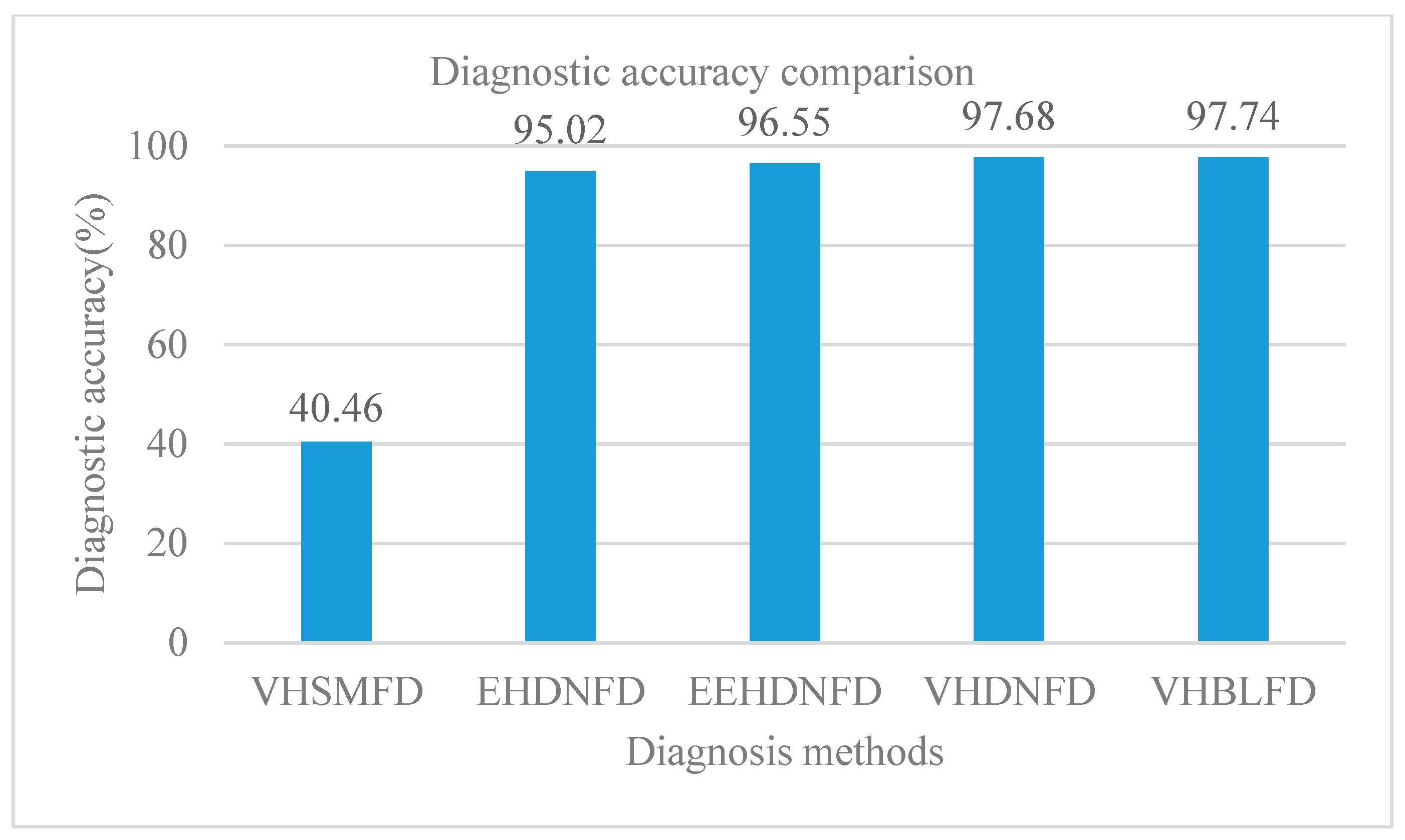
4.4. Comparision and Analysis for Diagnosis Results

In order to test and verify the effectiveness of the proposed VHSMFD method for rolling bearings of the AC motor, the VHSMFD method based on VMD, HT, and SVM, the EHDNFD method based on EMD, HT, and DBN, the EEHDNFD based on EEMD, HT and DBN, the VHDNFD method based on VMD, HT and DBN are compared with the proposed VHSMFD method. The four limited Boltzmann machines are used in this paper according to many experiments, that is, the five layer DBN, which allows for the shorter training time and obtain good diagnosis results. The number of nodes of the DBN (50-50-200) and the BLM (100-15-17,000) are set in this experiment. The initial values of parameters for SVM are described as c = 380, g = 0.4710, and p = 0.010375. The values of other parameters are the same as those in Section 4.3. The diagnosis results and the test times of different methods are shown in Table 3, Figure 7, and Figure 8.
From Table 3, Figure 7, and Figure 8, the diagnosis accuracies of VHSMFD, EHDNFD, EEHDNFD, VHDNFD, and VHBLFD are 40.46%, 95.02%, 96.55%, 97.68%, and 97.74%, respectively. For the VHSMFD method based on VMD, HT and SVM, the fault diagnosis accuracy is only 40.46%, and the diagnosis effect is the worst of the five diagnosis methods. The results show that the SVM cannot construct a fault diagnosis model with strong generalization ability for difference data. For the VHBLFD method, the diagnosis accuracy is 97.74%, and the diagnosis effect is better than that of the VHSMFD, EHDNFD, EEHDNFD and VHDNFD methods. The results show that the BLM can construct a fault diagnosis model with strong generalization ability and the higher accuracy for difference data. The test time of the VHSMFD, EHDNFD, EEHDNFD, VHDNFD and VHBLFD are 274.71 s, 664.57 s, 630.37, 459.21 s, and 22.29 s, respectively. The test times of EEHDNFD method is 664.57 s, and he fault diagnosis efficiency is the lowest of these diagnosis methods. The test time of the VHBLFD is 22.29 s, and the fault diagnosis efficiency is the highest of these fault diagnosis methods. The results show that the BLM can construct a fault diagnosis model with better diagnosis efficiency and faster diagnosis speed. Therefore, the VHBLFD takes on the higher diagnosis accuracy and better diagnosis efficiency.

4.5. The Influences of Parameters in BLM for Diagnosis Accuracy

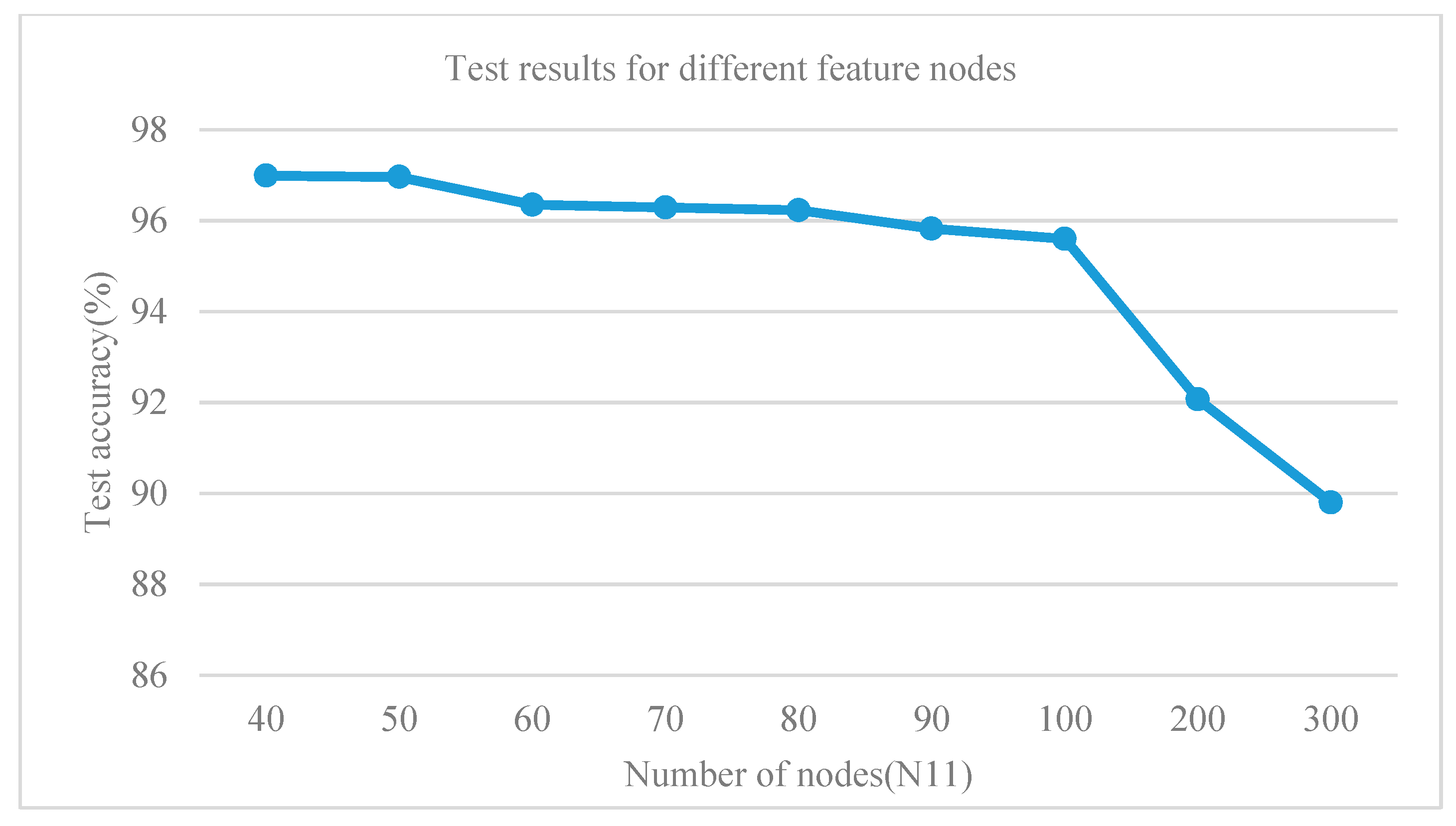
4.5.1. The Influences of the Number of Feature Nodes for Diagnosis Accuracy

In this section, when the number of feature node windows and the number of enhancement nodes are unchanged, the number of feature nodes is changed, and ten different states of the rolling bearings are identified. The experiment under each parameter is carried out ten times, and the test results and the running times are averaged for 10 times. The test results and running time are shown in Table 4, Figure 9, and Figure 10. The regularization parameter C is 2 × 10⁻³⁰, and the enhance node reduction ratio s is 0.8 in Table 1. N11 is the number of feature nodes. N2 is the number of feature node windows. N33 is the number of enhancement nodes.
From Table 4, Figure 9 and Figure 10, the total test time increases from 4.8618 s to 21.7082 s in the process of increasing feature nodes from 40 to 300, but the test accuracy takes on a decreasing trend from 96.9902% to 89.7968%. The experiment results show that the number of feature nodes can be reasonably selected according to the size of the input data in order to obtain the best diagnosis result in practical applications.

4.5.2. The Influences of the Number of Feature Node Windows for Diagnosis Accuracy

In this section, when the number of enhancement nodes and feature nodes is unchanged, the number of feature node windows is changed, and ten different states of the rolling bearings are identified. The experiment under each parameter is carried out ten times, and the test results and are running times are averaged for 10 times. The results and the running times are shown in Table 4, Figure 11, and Figure 12. The regularization parameter C is 2 × 10⁻³⁰, and the enhance node reduction ratio s is 0.8 in Table 5.
As can be seen from Table 5, Figure 11, and Figure 12, in the case of only changing the number of feature node windows, the total test time increases from 3.4090 s to 35.2004 s in the process of increasing feature windows from 5 to 90, and the test accuracy almost remains unchanged. The experimental results show that the training time of BLM is affected, and the test accuracy is less affected by the number of feature node windows. Therefore, the number of feature node windows only affects the training time of BLM.

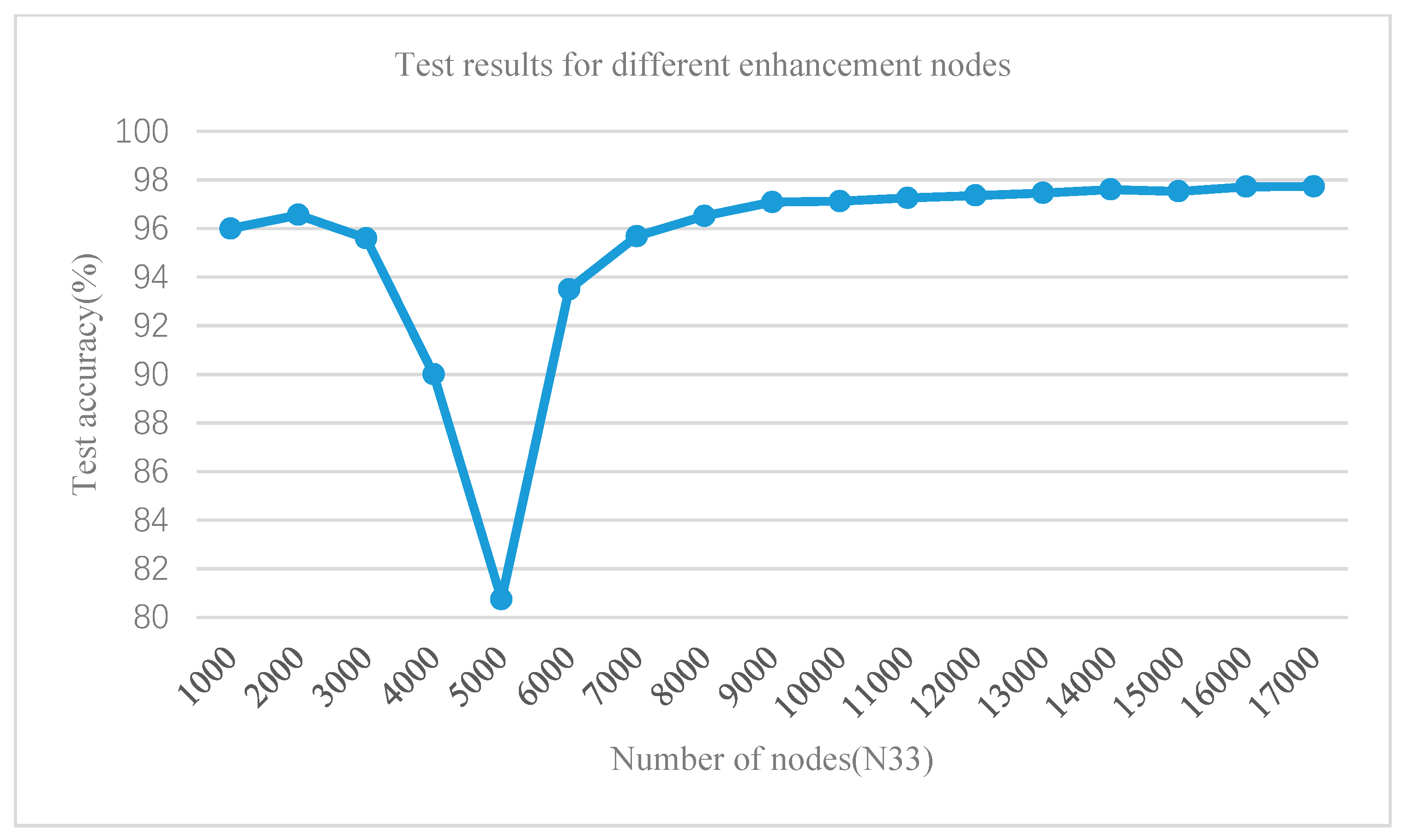
4.5.3. The Influences of the Number of Enhancement Nodes for Diagnosis Accuracy

In this section, when the number of feature nodes and feature node windows is unchanged, the number of enhancement nodes is changed, and ten different states of the bearing are identified. The experiment under each parameter is carried out ten times, and the test results and the running times are averaged for 10 times. The results and running time are shown in Table 6, Figure 13, and Figure 14. The regularization parameter C is 2 × 10⁻³⁰, and the enhance node reduction ratio s is 0.8 in Table 6.
As can be seen from Table 6, Figure 13, and Figure 14, in the case of changing only the number of the enhancement nodes, the training time of the BLM increases with the increase enhancement nodes. Under the influence of eliminating some special nodes, the test accuracy will also increase with the increasing of the enhancement nodes. The experiment results show that the number of enhancement nodes can be flexibly selected according to the different requirements of the BLM for training time and test accuracy. Therefore, the number of enhancement nodes not only affects the training time but also affects the test accuracy.
To sum up, the feature nodes and enhancement nodes can influence the accuracy of fault diagnosis, and the number of feature node windows cannot influence the accuracy using the BLM for fault diagnosis. Using the BLM for classifying the fault provide better diagnosis efficiency and faster diagnosis speed.

5. Conclusions

To effectively diagnose the faults of rolling bearings of the AC motor, a new fault diagnosis (VHBLFD) method based on VMD, HT, and BLM is proposed. VMD and HT are used to obtain Hilbert envelope spectra. The BLM is an effective incremental learning model to achieve competitive results of the state-of-art method. The BLM with fast calculation speed and strong generalization ability is used to realize the fault classification. The actual vibration data are used to validate the effectiveness of the VHBLFD. The fault diagnosis accuracy of the VHBLFD is 97.74%, and the test time of the VHBLFD is 22.29s. The results show that the BLM can construct the VHBLFD model with a higher diagnosis accuracy and a better diagnosis efficiency. Compared with the DBN and the SVM, the BLM is more sensitive for fault features and has faster diagnosis speed and better robustness. Therefore, the VHBLFD method provides higher diagnosis accuracy and better diagnosis efficiency.
In order to solve the practical engineering problem, we plan to design a new experiment platform to obtain a new dataset containing much more data. We will use the new dataset to study the fault diagnosis method in future work.

Author Contributions

Methodology, H.Z. and J.Z.; validation, L.Z.; resources, C.G.; data curation, W.D. and Y.Y.; writing—original draft preparation, J.Z. and Y.Y.; writing—review and editing, W.D.; visualization, L.Z.; funding acquisition, H.Z., W.D. and C.G.

Funding

This research was funded by the National Natural Science Foundation of China grant number 51605068, grant number 61771087, grant number 51879027, grant number 51579024, the Open Project Program of State Key Laboratory of Mechanical Transmissions of Chongqing University grant number SKLMT-KFKT-201803, Open Project Program of the Traction Power State Key Laboratory of Southwest Jiaotong University under Grant TPL1803, and Liaoning BaiQianWan Talents Program.

Conflicts of Interest

The authors declare no conflict of interest.

References

  1. Lu, S.L.; He, Q.B.; Zhang, H.B.; Kong, F.R. Rotating machine fault diagnosis through enhancement stochastic resonance by full-wave signal construction. Mech. Syst. Signal Process. 2017, 85, 82–97. [Google Scholar] [CrossRef]
  2. Yang, Y.; Yu, D.J.; Cheng, J.S. A fault diagnosis approach for roller bearing based on IMF envelope spectrum and SVM. Measurement 2007, 40, 943–950. [Google Scholar] [CrossRef]
  3. Deng, W.; Zhang, S.J.; Zhao, H.M.; Yang, X.H. A novel fault diagnosis method based on integrating empirical wavelet transform and fuzzy entropy for motor bearing. IEEE Access 2018, 6, 35042–35056. [Google Scholar] [CrossRef]
  4. Guo, S.K.; Chen, R.; Wei, M.M.; Li, H.; Liu, Y.Q. Ensemble data reduction techniques and Multi-RSMOTE via fuzzy integral for bug report classification. IEEE Access 2018, 6, 45934–45950. [Google Scholar] [CrossRef]
  5. Yu, J.; Ding, B.; He, Y.J. Rolling bearing fault diagnosis based on mean multigranulation decision-theoretic rough set and non-naive Bayesian classifier. J. Mech. Sci. Technol. 2018, 32, 5201–5211. [Google Scholar] [CrossRef]
  6. Liu, Y.Q.; Yi, X.K.; Chen, R.; Zhai, Z.G.; Gu, J.X. Feature extraction based on information gain and sequential pattern for English question classification. IET Softw. 2018, 12, 520–526. [Google Scholar] [CrossRef]
  7. Deng, W.; Yao, R.; Zhao, H.M.; Yang, X.H.; Li, G.Y. A novel intelligent diagnosis method using optimal LS-SVM with improved PSO algorithm. Soft Comput. 2019, 23, 2445–2462. [Google Scholar] [CrossRef]
  8. Ren, Z.R.; Skjetne, R.; Jiang, Z.Y.; Gao, Z.; Verma, A.S. Integrated GNSS/IMU hub motion estimator for offshore wind turbine blade installation. Mech. Syst. Signal Process. 2019, 123, 222–243. [Google Scholar] [CrossRef]
  9. Chen, H.L.; Xu, Y.T.; Wang, M.J.; Zhao, X.H. Chaos-induced and Mutation-driven algorithm for constrained engineering design problems. Appl. Math. Model. 2019, 71, 45–59. [Google Scholar] [CrossRef]
  10. Lu, S.L.; Zhou, P.; Wang, X.X.; Liu, B.Y.; Liu, F.; Zhao, J.W. Condition monitoring and fault diagnosis of motor bearings using undersampled vibration signals from a wireless sensor network. J. Sound Vib. 2018, 414, 81–96. [Google Scholar] [CrossRef]
  11. Xie, H.M.; Yang, K.; Li, S.W.; Yin, S.; Peng, J.; Zhu, F.; Li, H.; Zhang, L. Microwave heating-assisted pyrolysis of mercury from sludge. Mater. Res. Express 2019, 6, 015507. [Google Scholar] [CrossRef]
  12. Deng, W.; Xu, J.J.; Zhao, H.M. An improved ant colony optimization algorithm based on hybrid strategies for scheduling problem. IEEE Access 2019, 7, 20281–20292. [Google Scholar] [CrossRef]
  13. Yu, J.; He, Y.J. Planetary gearbox fault diagnosis based on data-driven valued characteristic multigranulation model with incomplete diagnostic information. J. Sound Vib. 2018, 429, 63–77. [Google Scholar] [CrossRef]
  14. Osman, S.; Wang, W. A normalized Hilbert-Huang transform technique for bearing fault detection. J. Vib. Control 2014, 22, 2771–2787. [Google Scholar] [CrossRef]
  15. Wang, L.H.; Zhao, X.P.; Wu, J.X.; Xie, Y.Y.; Zhang, Y.H. Motor fault diagnosis based on short-time Fourier transform and convolutional neural network. Chin. J. Mech. Eng. 2017, 30, 1357–1368. [Google Scholar] [CrossRef]
  16. Pan, Y.N.; Chen, J. The changes of complexity in the performance degradation process of rolling element bearing. J. Vib. Control 2016, 22, 344–357. [Google Scholar] [CrossRef]
  17. Li, T.; Hu, Z.; Jia, Y.; Wu, J.; Zhou, Y. Forecasting crude oil prices using ensemble empirical mode decomposition and sparse Bayesian learning. Energies 2018, 11, 1882. [Google Scholar] [CrossRef]
  18. Ren, Z.; Skjetne, R.; Gao, Z. A crane overload protection controller for blade lifting operation based on model predictive control. Energies 2019, 12, 50. [Google Scholar] [CrossRef]
  19. Liu, G.; Chen, B.; Jiang, S.; Fu, H.; Wang, L.; Jiang, W. Double entropy joint distribution function and its application in calculation of design wave height. Entropy 2019, 21, 64. [Google Scholar] [CrossRef]
  20. Zhao, H.M.; Sun, M.; Deng, W.; Yang, X.H. A new feature extraction method based on EEMD and multi-scale fuzzy entropy for motor bearing. Entropy 2017, 19, 14. [Google Scholar] [CrossRef]
  21. Chen, R.; Guo, S.K.; Wang, X.Z.; Zhang, T.L. Fusion of multi-RSMOTE with fuzzy integral to classify bug reports with an imbalanced distribution. IEEE Trans. Fuzzy Syst. 2019. [Google Scholar] [CrossRef]
  22. Zhao, H.M.; Yao, R.; Xu, L.; Yuan, Y.; Li, G.Y.; Deng, W. Study on a novel fault damage degree identification method using high-order differential mathematical morphology gradient spectrum entropy. Entropy 2018, 20, 682. [Google Scholar] [CrossRef]
  23. Sun, F.R.; Yao, Y.D.; Li, X.F. The heat and mass transfer characteristics of superheated steam coupled with non-condensing gases in horizontal wells with multi-point injection technique. Energy 2018, 143, 995–1005. [Google Scholar] [CrossRef]
  24. Guo, S.K.; Chen, R.; Li, H.; Zhang, T.L.; Liu, Y.Q. Identify severity bug report with distribution imbalance by CR-SMOTE and ELM. Int. J. Softw. Eng. Knowl. Eng. 2019, 29, 139–175. [Google Scholar] [CrossRef]
  25. Zhou, Y.R.; Li, T.Y.; Shi, J.Y.; Qian, Z.J. A CEEMDAN and XGBOOST–based approach to forecast crude oil prices. Complexity 2019. [Google Scholar] [CrossRef]
  26. Deng, W.; Zhao, H.M.; Yang, X.H.; Xiong, J.X.; Sun, M.; Li, B. Study on an improved adaptive PSO algorithm for solving multi-objective gate assignment. Appl. Soft Comput. 2017, 59, 288–302. [Google Scholar] [CrossRef]
  27. Guo, J.H.; Mu, Y.; Xiong, M.D.; Liu, Y.Q.; Gu, J.X. Activity feature solving based on TF-IDF for activity recognition in smart homes. Complexity 2019. [Google Scholar] [CrossRef]
  28. Fu, H.; Li, Z.; Liu, Z.; Wang, Z. Research on big data digging of hot topics about recycled water use on micro-blog based on particle swarm optimization. Sustainability 2018, 10, 2488. [Google Scholar] [CrossRef]
  29. Tang, G.; Zhang, Y.; Wang, H.Q. Multivariable LS-SVM with moving window over time slices for the prediction of bearing performance degradation. J. Intell. Fuzzy Syst. 2018, 34, 3747–3757. [Google Scholar] [CrossRef]
  30. Kim, K.J.; Cho, S.B. Ensemble Bayesian networks evolved with speciation for high-performance prediction in data mining. Soft Comput. 2017, 21, 1065–1080. [Google Scholar] [CrossRef]
  31. Deng, W.; Zhao, H.M.; Zou, L.; Li, G.Y.; Yang, X.H.; Wu, D.Q. A novel collaborative optimization algorithm in solving complex optimization problems. Soft Comput. 2017, 21, 4387–4398. [Google Scholar] [CrossRef]
  32. Wang, H.C.; Chen, J. Performance degradation assessment of rolling bearing based on bispectrum and support vector data description. J. Vib. Control 2014, 20, 2032–2041. [Google Scholar] [CrossRef]
  33. Yu, J.; Bai, M.Y.; Wang, G.N.; Shi, X.J. Fault diagnosis of planetary gearbox with incomplete information using assignment reduction and flexible naive Bayesian classifier. J. Mech. Sci. Technol. 2018, 32, 37–47. [Google Scholar] [CrossRef]
  34. Gao, H.Z.; Liang, L.; Chen, X.G.; Xu, G.H. Feature extraction and recognition for rolling element bearing fault utilizing short-time Fourier transform and non-negative matrix factorization. Chin. J. Mech. Eng. 2015, 28, 96–105. [Google Scholar] [CrossRef]
  35. Zhang, C.L.; Li, B.; Chen, B.Q.; Cao, H.; Zi, Y.; He, Z. Weak fault signature extraction of rotating machinery using flexible analytic wavelet transform. Mech. Syst. Signal. Process. 2015, 64, 162–187. [Google Scholar] [CrossRef]
  36. Kabla, A.; Mokrani, K. Bearing fault diagnosis using Hilbert-Huang transform (HHT) and support vector machine (SVM). Mech. Ind. 2016, 17, 308. [Google Scholar] [CrossRef]
  37. Yuan, J.; Ji, F.; Gao, Y.; Zhu, J.; Wei, C.; Zhou, Y. Integrated ensemble noise-reconstructed empirical mode decomposition for mechanical fault detection. Mech. Syst. Signal Process. 2018, 104, 323–346. [Google Scholar] [CrossRef]
  38. Du, Y.C.; Du, D.P. Fault detection and diagnosis using empirical mode decomposition based principal component analysis. Comput. Chem. Eng. 2018, 115, 1–21. [Google Scholar] [CrossRef]
  39. Fei, S.W.; He, Y. A multi-layer KMC-RS-SVM classifier and DGA for fault diagnosis of power transformer. Recent Pat. Comput. Sci. 2012, 5, 238–243. [Google Scholar] [CrossRef]
  40. Kang, L.; Zhao, L.; Yao, S.; Duan, C.X. A new architecture of super-hydrophilic β-SiAlON/graphene oxide ceramic membrane for enhanced anti-fouling and separation of water/oil emulsion. Ceram. Int. 2019. [Google Scholar] [CrossRef]
  41. Cheng, J.S.; Peng, Y.F.; Yang, Y.; Wu, Z. Adaptive sparsest narrow-band decomposition method and its applications to rolling element bearing fault diagnosis. Mech. Syst. Signal Process. 2017, 85, 947–962. [Google Scholar] [CrossRef]
  42. Huang, W.Y.; Cheng, J.S.; Yang, Y. Rolling bearing performance degradation assessment based on convolutional sparse combination learning. IEEE Access 2019, 7, 17834–17846. [Google Scholar] [CrossRef]
  43. Huang, W.Y.; Cheng, J.S.; Yang, Y. Rolling bearing fault diagnosis and performance degradation assessment under variable operation conditions based on nuisance attribute projection. Mech. Syst. Signal Process. 2019, 114, 165–188. [Google Scholar] [CrossRef]
  44. Van Tung, T.; AlThobiani, F.; Ball, A. An approach to fault diagnosis of reciprocating compressor valves using Teager-Kaiser energy operator and deep belief networks. Expert Syst. Appl. 2014, 41, 4113–4122. [Google Scholar]
  45. Guo, X.J.; Chen, L.; Shen, C.Q. Hierarchical adaptive deep convolution neural network and its application to bearing fault diagnosis. Measurement 2016, 93, 490–502. [Google Scholar] [CrossRef]
  46. Qi, Y.M.; Shen, C.Q.; Wang, D.; Shi, J.; Jiang, X.; Zhu, Z. Stacked sparse autoencoder-based deep network for fault diagnosis of rotating machinery. IEEE Access 2017, 5, 15066–15079. [Google Scholar] [CrossRef]
  47. Shao, H.D.; Jiang, H.K.; Wang, F.A.; Wang, Y. Rolling bearing fault diagnosis using adaptive deep belief network with dual-tree complex wavelet packet. ISA Trans. 2017, 69, 187–201. [Google Scholar] [CrossRef]
  48. Li, S.B.; Liu, G.K.; Tang, X.H.; Lu, J.; Hu, J. An ensemble deep convolutional neural network model with improved d-s evidence fusion for bearing fault diagnosis. Sensors 2017, 17, 1729. [Google Scholar] [CrossRef]
  49. Shao, H.D.; Jiang, H.K.; Zhang, H.Z.; Duan, W.; Liang, T.; Wu, S. Rolling bearing fault feature learning using improved convolutional deep belief network with compressed sensing. Mech. Syst. Signal Process. 2018, 100, 743–765. [Google Scholar] [CrossRef]
  50. Sun, C.; Ma, M.; Zhao, Z.B.; Chen, X.F. Sparse deep stacking network for fault diagnosis of motor. IEEE Trans. Ind. Inform. 2018, 14, 3261–3270. [Google Scholar] [CrossRef]
  51. Zhang, W.; Li, C.H.; Peng, G.L.; Chen, Y.; Zhang, Z. A deep convolutional neural network with new training methods for bearing fault diagnosis under noisy environment and different working load. Mech. Syst. Signal Process. 2018, 100, 439–453. [Google Scholar] [CrossRef]
  52. Shao, H.D.; Jiang, H.K.; Zhang, H.Z.; Liang, T. Electric locomotive bearing fault diagnosis using a novel convolutional deep belief network. IEEE Trans. Ind. Electron. 2018, 65, 2727–2736. [Google Scholar] [CrossRef]
  53. Wang, Z.R.; Wang, J.; Wang, Y.R. An intelligent diagnosis scheme based on generative adversarial learning deep neural networks and its application to planetary gearbox fault pattern recognition. Neurocomputing 2018, 310, 213–222. [Google Scholar] [CrossRef]
  54. Wang, S.H.; Xiang, J.W.; Zhong, Y.T.; Tang, H. A data indicator-based deep belief networks to detect multiple faults in axial piston pumps. Mech. Syst. Signal Process. 2018, 112, 154–170. [Google Scholar] [CrossRef]
  55. Liu, H.; Zhou, J.Z.; Xu, Y.H.; Zheng, Y.; Peng, X.; Jiang, W. Unsupervised fault diagnosis of rolling bearings using a deep neural network based on generative adversarial networks. Neurocomputing 2018, 315, 412–424. [Google Scholar] [CrossRef]
  56. Zhao, X.L.; Jia, M.P. A novel deep fuzzy clustering neural network model and its application in rolling bearing fault recognition. Meas. Sci. Technol. 2018, 29, 125005. [Google Scholar] [CrossRef]
  57. Hu, Z.X.; Jiang, P. An imbalance modified deep neural network with dynamical incremental learning for chemical fault diagnosis. IEEE Trans. Ind. Electron. 2019, 66, 540–550. [Google Scholar] [CrossRef]
  58. Li, Z.P.; Chen, J.L.; Zi, Y.Y.; Pan, J. Independence-oriented VMD to identify fault feature for wheel set bearing fault diagnosis of high speed locomotive. Mech. Syst. Signal Process. 2017, 85, 512–529. [Google Scholar] [CrossRef]
  59. Jiang, X.X.; Shen, C.Q.; Shi, J.J.; Zhu, Z. Initial center frequency-guided VMD for fault diagnosis of rotating machines. J. Sound Vib. 2018, 435, 36–55. [Google Scholar] [CrossRef]
  60. Li, J.M.; Yao, X.F.; Wang, H.; Zhang, J. Periodic impulses extraction based on improved adaptive VMD and sparse code shrinkage denoising and its application in rotating machinery fault diagnosis. Mech. Syst. Signal Process. 2019, 126, 568–589. [Google Scholar] [CrossRef]
  61. Wang, C.G.; Li, H.K.; Huan, G.J.; Ou, J. Early fault diagnosis for planetary gearbox based on adaptive parameter optimized VMD and singular kurtosis difference spectrum. IEEE Access 2019, 7, 31501–31516. [Google Scholar] [CrossRef]
  62. Zhang, F.Q.; Lei, T.S.; Li, J.H.; Cai, X.; Shao, X.; Chang, J.; Tian, F. Real-time calibration and registration method for indoor scene with joint depth and color camera. J. Pattern Recognit. Artif. Intell. 2018, 32, 1854021. [Google Scholar] [CrossRef]
  63. Guo, S.K.; Liu, Y.Q.; Chen, R.; Sun, X.; Wang, X.X. Using an improved SMOTE algorithm to deal imbalanced activity classes in smart home. Neural Process. Lett. 2018. [Google Scholar] [CrossRef]
  64. Wen, J.; Zhong, Z.F.; Zhang, Z.; Fei, L.K.; Lai, Z.H.; Chen, R.Z. Adaptive locality preserving regression. IEEE Trsns. Circ. Syst. Vid. 2018. [Google Scholar] [CrossRef]
  65. Liu, Y.Q.; Wang, X.X.; Zhai, Z.G.; Chen, R.; Zhang, B.; Jiang, Y. Timely daily activity recognition from headmost sensor events. ISA Trans. 2019. [Google Scholar] [CrossRef] [PubMed]
  66. Zhang, F.Q.; Wang, Z.W.; Chang, J.; Zhang, J.; Tian, F. A fast framework construction and visualization method for particle-based fluid. EUPASIP J. Image Video Process. 2017, 2017, 79. [Google Scholar] [CrossRef] [Green Version]
  67. Huang, F.; Yao, C.; Liu, W.; Li, Y.; Liu, X. Landslide susceptibility assessment in the nantian area of china: A comparison of frequency ratio model and support vector machine. Geomat. Nat. Haz. Risk 2018, 9, 919–938. [Google Scholar] [CrossRef]
  68. Zhang, H.; Fang, Y. Temperature dependent photoluminescence of surfactant assisted electrochemically synthesized ZnSe nanostructures. J. Alloy Compd. 2019, 781, 201–208. [Google Scholar] [CrossRef]
  69. Liu, G.; Chen, B.; Gao, Z.; Fu, H.; Jiang, S.; Wang, L.; Yi, K. Calculation of joint return period for connected edge data. Water 2019, 11, 300. [Google Scholar] [CrossRef]
  70. Zhou, J.; Du, Z.; Yang, Z.; Xu, Z. Dynamic parameters optimization of straddle-type monorail vehicles based multiobjective collaborative optimization algorithm. Vehicle Syst. Dyn. 2019. [Google Scholar] [CrossRef]
  71. Lin, J.; Yuan, J.S. Analysis and simulation of capacitor-less ReRAM-based stochastic neurons for the in-memory spiking neural network. IEEE Trans. Biomed Circ. Syst. 2018, 12, 1004–1017. [Google Scholar] [CrossRef] [PubMed]
  72. Wen, J.; Fang, X.Z.; Cui, J.R.; Fei, L.K.; Yan, K.; Chen, Y.; Xu, Y. Robust sparse linear discriminant analysis. IEEE Trans. Circ. Syst. Vid. 2019, 29, 390–403. [Google Scholar] [CrossRef]
  73. Chen, H.L.; Jiao, S.; Heidarib, A.A.; Wang, M.J.; Chen, X.; Zhao, X.H. An opposition-based sine cosine approach with local search for parameter estimation of photovoltaic models. Energ. Convers. Manage. 2019, 195, 927–942. [Google Scholar] [CrossRef]
  74. Yu, W.J.; Zeng, Z.; Peng, B.; Yan, S.; Huang, Y.H.; Jiang, H.; Li, X.B.; Fan, T. Multi-objective optimum design of high-speed backplane connector using particle swarm optimization. IEEE Access 2018, 6, 35182–35193. [Google Scholar] [CrossRef]
  75. Luo, J.; Chen, H.L.; Zhang, Q.; Xu, Y.T.; Huang, H.; Zhao, X.H. An improved grasshopper optimization algorithm with application to financial stress prediction. Appl. Math. Model. 2018, 64, 654–668. [Google Scholar] [CrossRef]
  76. Liu, G.; Gao, Z.; Chen, B.; Fu, H.; Jiang, S.; Wang, L.; Koi, Y. Study on Threshold selection methods in calculation of ocean environmental design parameters. IEEE ACCESS 2019, 7, 39515–39527. [Google Scholar] [CrossRef]
  77. Hinton, G.E.; Osindero, S.; Teh, Y.W. A fast learning algorithm for deep belief nets. Neural Comput. 2006, 18, 1527–1554. [Google Scholar] [CrossRef] [PubMed]
  78. Chen, C.P.; Liu, Z.L. Broad learning system: An effective and efficient incremental learning system without the need for deep architecture. IEEE Trans. Neural Netw. Learn. Syst. 2018, 29, 10–24. [Google Scholar] [CrossRef]
  79. Bearing Data Center. Available online: http://csegroups.case.edu/bearingdatacenter/home (accessed on 13 July 2017).
Figure 1. Structure of RBM.
Symmetry 11 00747 g001
Figure 2. The broad learning model.
Symmetry 11 00747 g002
Figure 3. The flow of fault diagnosis method.
Symmetry 11 00747 g003
Figure 4. The experiment platform.
Symmetry 11 00747 g004
Figure 5. Decomposition of inner race fault signal.
Symmetry 11 00747 g005
Figure 6. The VMD-Hilbert envelope spectra for different fault data.
Symmetry 11 00747 g006
Figure 7. The comparison results of diagnostic accuracy.
Symmetry 11 00747 g007
Figure 8. The comparison results of test time.
Symmetry 11 00747 g008
Figure 9. The test accuracy of different numbers of nodes (N11).
Symmetry 11 00747 g009
Figure 10. The total average times of different numbers of nodes (N11).
Symmetry 11 00747 g010
Figure 11. The test accuracy of different numbers of nodes (N2).
Symmetry 11 00747 g011
Figure 12. The total average time of different numbers of nodes (N2).
Symmetry 11 00747 g012
Figure 13. The test accuracy of different numbers of nodes (N33).
Symmetry 11 00747 g013
Figure 14. The total average times of different numbers of nodes (N33).
Symmetry 11 00747 g014
Table 1. The sample data.
No.Inner RaceOuter RaceRolling Element
1−0.08300.0085−0.0028
2−0.19570.4235−0.0963
30.23340.01300.1137
40.1040−0.26520.2573
5−0.18110.2372−0.0583
60.05560.5909−0.1260
70.1738−0.09300.2074
8−0.0469−0.40690.1727
9−0.11190.2794−0.2199
100.05960.4370−0.1561
110−0.35290.2240
20410.23050.03090.2375
20420.04610.1186−0.0271
2043−0.5122−0.0061−0.1327
20440.1481−0.09790.0929
20450.62800.09140.1106
2046−0.20430.1494−0.1499
2047−0.2640−0.2355−0.1108
20480.4662−0.32240.1467
Table 2. The diagnosis results and test times of the proposed VHBLFD method.
Fault Diagnosis MethodDiagnostic Accuracy (%)Test Time (s)
VHBLFD1 (100,5,1000)95.996.45
VHBLFD2 (100,15,17000)97.7422.29
Table 3. Comparison of diagnosis results and test time.
Diagnosis MethodsDiagnostic Accuracy (%)Test Time (s)
VHSMFD40.46274.71
EHDNFD95.02664.57
EEHDNFD96.55630.37
VHDNFD97.68459.21
VHBLFD97.7422.29
Table 4. Test results for different feature nodes. (N11 is the number of feature nodes, N2 is the number of feature node windows, and N33 is the number of enhancement nodes).
(N11, N2, N33)Test Accuracy (%)Total Average Time (s)
40, 15, 300096.99024.8618
50, 15, 300096.96015.2248
60, 15, 300096.35065.6163
70, 15, 300096.29046.0630
80, 15, 300096.23026.5115
90, 15, 300095.82397.0634
100, 15, 300095.59827.5683
200, 15, 300092.069215.0772
300, 15, 300089.796821.7082
Table 5. Test results for different feature node windows.
Number of Nodes (N11, N2, N33)Test Accuracy (%)Total Average Time (s)
100, 5, 100095.82393.4090
100, 10, 100095.77874.9404
100, 15, 100095.94436.4226
100, 20, 100095.98197.9057
100, 25, 100095.91429.4303
100, 30, 100096.079710.9200
100, 35, 100095.673412.4819
100, 40, 100095.7035 14.1060
100, 45, 100095.786315.8277
100, 50, 100095.756217.6226
100, 55, 100095.477819.6315
100, 60, 100095.741120.9249
100, 65, 100095.635822.5161
100, 70, 100095.771224.0979
100, 75, 100095.665935.2004
100, 80, 100095.477826.8084
100, 85, 100095.530428.5762
100, 90, 100095.635830.5728
Table 6. Test results for different enhancement nodes.
Number of Nodes (N11, N2, N33)Test Accuracy (%)Total Average Time (s)
100, 15, 100095.99706.4500
100, 15, 200096.56137.1869
100, 15, 300095.59827.5683
100, 15, 400090.00008.0937
100, 15, 500080.73748.9812
100, 15, 600093.49899.2012
100, 15, 700095.68109.9691
100, 15, 800096.516210.7368
100, 15, 900097.088011.6575
100, 15, 1000097.125712.7143
100, 15, 1100097.261113.6536
100, 15, 1200097.358914.8280
100, 15, 1300097.464316.0800
100, 15, 1400097.607217.3710
100, 15, 1500097.532018.6380
100, 15, 1600097.720020.8649
100, 15, 1700097.735122.2932

