Article

Compression of a Polar Orthotropic Wedge between Rotating Plates: Distinguished Features of the Solution

1
School of Mechanical Engineering and Automation, Beihang University, Beijing 100191, China
2
Russian Academy of Sciences, Ishlinsky Institute for Problems in Mechanics RAS, 101-1 Prospect Vernadskogo, 119526 Moscow, Russia
3
Vietnam Academy of Science and Technology, Institute of Mechanics, Hanoi 264 Doi Can, Vietnam
*
Author to whom correspondence should be addressed.
Symmetry 2019, 11(2), 270; https://doi.org/10.3390/sym11020270
Submission received: 29 January 2019 / Revised: 19 February 2019 / Accepted: 19 February 2019 / Published: 20 February 2019

Abstract

:
An infinite wedge of orthotropic material is confined between two rotating planar rough plates, which are inclined at an angle 2α. An instantaneous boundary value problem for the flow of the material is formulated and solved for the stress and the velocity fields, the solution being in closed form. The solution may exhibit the regimes of sliding or sticking at the plates. It is shown that the overall structure of the solution significantly depends on the friction stress at sliding. This stress is postulated by the friction law. Solutions, which exhibit sticking, may exist only if the postulated friction stress at sliding satisfies a certain condition. These solutions have a rigid rotating zone in the region adjacent to the plates, unless the angle α is equal to a certain critical value. Solutions which exhibit sliding may be singular. In particular, some space stress and velocity derivatives approach infinity in the vicinity of the friction surface.

1. Introduction

An instantaneous plane strain rigid plastic solution is obtained for compression of an infinite wedge of orthotropic material confined between two rough plates, inclined at angle 2α, and which intersect in a line. This boundary value problem is ideal for studying qualitative mathematical properties of boundary value problems, including constitutive equations and boundary conditions. For, exact analytical or semi-analytical solutions can be found for many constitutive equations. In particular, such solutions have been presented in [1,2] for isotropic viscoplastic materials and in [3] for the double slip and rotation model. A description of this model can be found in [4].
The present paper provides an analytic solution for rigid plastic orthotropic material. It is assumed that the principal axes of anisotropy are straight lines through the apex of the wedge and orthogonal curves, which are of course circular arcs. This type of orthotropy is of practical interest [5,6,7,8] among many others. The paper focuses on qualitative features of the solution such as non-existence of the solution, singularity in the stress and velocity fields, appearance of a rigid region near the plates and transition between the regimes of sticking and sliding. The effect of plastic anisotropy on these features is discussed.
The stress and velocity fields are singular if the regime of sliding occurs in the case of the maximum friction law. A detailed asymptotic analysis of the solution is performed for this case. In particular, it is shown that the asymptotic behavior of the solution is in agreement with the general theory developed in [9].
An applied aspect of the solution found, is that it can be used in conjunction with the method for analysis and the design of flat-rolling proposed in [10]. It is known that solutions, found by means of this method, show a good comparison with experiment [11,12,13], and are used for verifying solutions found by means of other approximate methods [14,15]. The importance of developing fast approximate methods for the analysis and design of the process of rolling has been emphasized in [16].

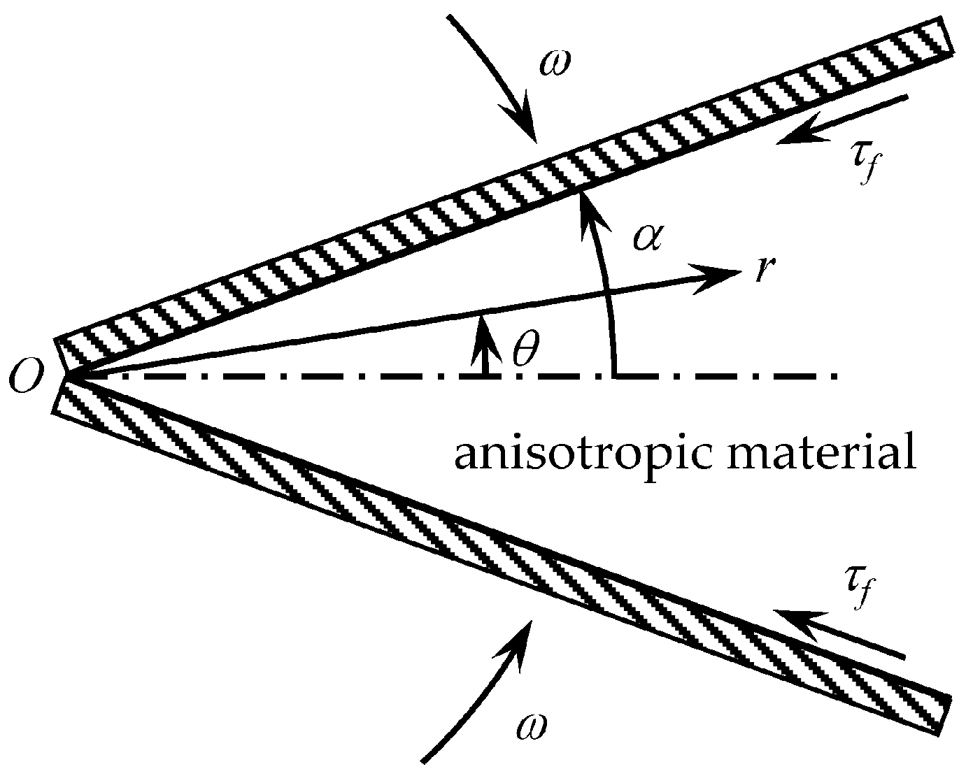
2. Statement of the Problem

Two semi-infinite rough plates rotate towards each other with angular velocity of magnitude ω about an axis O and compress a wedge of polar orthotropic material. The plates are inclined to each other at an angle 2α (Figure 1). The boundary value problem consists of the instantaneous plane strain deformation of the wedge. The problem is solved in a system of plane polar coordinates ( r , θ ) with its origin at O and with θ = 0 , taken as the perpendicular bisector of the angle 2α. It is assumed that the principal axes of anisotropy coincide with coordinate curves of the coordinate system chosen. Then, θ = 0 is an axis of symmetry for the flow and it is sufficient to find the solution in the region θ 0 . The components of the stress tensor referred to the polar coordinate system are denoted as σ r r , σ θ θ and σ r θ ; and the components of the velocity vector as u r and u θ . There is no material flux through O.
Therefore, the radial velocity should satisfy the following condition:
u r = 0
at r = 0 . By symmetry,
u θ = 0
and
σ r θ = 0
at θ = 0 . The circumferential velocity should also satisfy the condition:
u θ = ω r
at θ = α . Finally, the friction law is taken in the form:
{ u r = 0 if | σ r θ | τ f σ r θ = τ f otherwise
at θ = α . Here τ f > 0 denotes the frictional stress at sliding. The magnitude of τ f will be specified later. The sense of σ r θ in (5) is dictated by the condition that u r 0 at the plate.
It is assumed that the material obeys Hill’s quadratic yield criterion [17] and its associated flow rule. The elastic portion of strain is neglected. In the case of plane strain deformation of a polar orthotropic material, whose principal axes of anisotropy coincide with the coordinate curves of the polar coordinate system, the constitutive equations of the model are:
( σ r r σ θ θ ) 2 4 ( 1 c ) + σ r θ 2 = T 2
and
ξ r r = λ ( σ r r σ θ θ ) 2 ( 1 c ) , ξ θ θ = λ ( σ r r σ θ θ ) 2 ( 1 c ) , ξ r θ = λ σ r θ
where (6) in the yield criterion and (7) is the associated flow rule. The quantity T is the shear yield stress in the coordinate system chosen, c is a constitutive parameter, λ is a non-negative multiplier, ξ r r , ξ θ θ , ξ r θ denote the components of the strain rate tensor. The parameter c can be expressed in terms of the yield stresses in the directions of the principal axes of anisotropy and can vary (theoretically) in the range < c < 1 [17]. Eliminating λ between the equations in (7) yields:
ξ r r + ξ θ θ = 0 , ξ r θ ξ r r ξ θ θ = ( 1 c ) σ r θ σ r r σ θ θ .
It is evident that the first equation here is the equation of incompressibility. The strain rate components are expressed in terms of the velocity components as
ξ r r = u r r   ,   ξ θ θ = 1 r u θ θ + u r r ,   ξ r θ = 1 2 ( 1 r u r θ + u θ r u θ r ) .
The system of Equations (6), (8) and (9) are supplemented by the stress equilibrium equations:
σ r r r + 1 r σ r θ θ + σ r r σ θ θ r = 0 , σ r θ r + 1 r σ θ θ θ + 2 σ r θ r = 0 .
In total, there are five unknowns (three components of the stress tensor and two components of the velocity vector). The equations to solve are (6), (8) and (10). It is understood here that the components of the strain rate tensor in (8) should be eliminated by means of (9). The solution should satisfy the conditions (1) to (5).

3. General Stress Solution

The yield criterion (6) is satisfied by the following substitution:
σ r r = σ + T 1 c cos 2 φ , σ θ θ = σ T 1 c cos 2 φ , σ r θ = T sin 2 φ
where σ and φ are new unknown functions of r and θ . The direction of flow dictates that σ r θ 0 and σ r r σ θ θ 0 . Then, it is immediate from (11) that:
0 φ π 4 .
Using (11) and (12) the boundary condition (3) transforms to:
φ = 0
at θ = 0 . Substituting (11) into (10) gives:
σ r 2 T 1 c sin 2 φ φ r 2 T cos 2 φ r φ θ + 2 T 1 c cos 2 φ r = 0 , 2 T cos 2 φ φ r + σ r θ 2 T 1 c sin 2 φ r φ θ 2 T sin 2 φ r = 0 .
A standard assumption made in similar problems of the classical theory of plasticity is that φ is independent of r [17]. In this case, the equations in (14) become:
σ r 2 T cos 2 φ r d φ d θ + 2 T 1 c cos 2 φ r = 0 , σ 2 T θ 1 c sin 2 φ d φ d θ sin 2 φ = 0 .
The first equation can be immediately integrated to give:
σ 2 T = ( d φ d θ 1 c ) cos 2 φ ln ( r r 0 ) + σ 0 ( θ ) 2 T .
Here r 0 is a constant introduced for convenience and σ 0 ( θ ) is an arbitrary function of θ . Substituting (16) into the second equation in (15) yields:
d d θ [ ( d φ d θ 1 c ) cos 2 φ ] ln ( r r 0 ) = 1 c sin 2 φ d φ d θ + sin 2 φ d σ 0 2 T d θ .
Since the right-hand side of this equation is independent of r, the coefficient of ln ( r / r 0 ) on the left-hand side must vanish. Then, Equation (17) results in the following two equations:
( d φ d θ 1 c ) cos 2 φ = K 0 1 c , d σ 0 2 T d θ = ( 1 c d φ d θ + 1 ) sin 2 φ .
Here K 0 is a constant of integration. Equation (16) becomes:
σ 2 T = K 0 1 c ln ( r r 0 ) + σ 0 ( θ ) 2 T .
The second equation in (18) can be rewritten as:
d σ 0 2 T d φ = ( 1 c + d θ d φ ) sin 2 φ .
Eliminating in this equation the derivative d θ / d φ by means of the first equation in (18) leads to:
d σ 0 2 T d φ = 1 1 c [ 1 c + cos 2 φ ( K 0 + cos 2 φ ) ] sin 2 φ .
Integrating gives:
σ 0 2 T = 1 2 1 c [ cos 2 φ + K 0 l n ( K 0 + cos 2 φ ) + K 1 ]
where K 1 is constant of integration.
It is seen from (12) and (13) that d φ / d θ > 0 at φ = 0 . Therefore, it follows from the first equation in (18) that
K 0 > 1 .
The first equation in (18) can be integrated to give:
θ 1 c = φ K 0 arctanh [ 1 K 0 1 + K 0 tan φ ] ( 1 K 0 2 ) 1 / 2
if | K 0 | < 1 ,
θ 1 c = φ K 0 arctan [ K 0 1 K 0 + 1 tan φ ] ( K 0 2 1 ) 1 / 2
if K 0 > 1 , and
θ 1 c = φ tan φ 2
if K 0 = 1 . The solution for an important special case of (22), K 0 = 0 , is represented as
θ 1 c = φ .
The constant K 0 cannot be determined without the solution for velocity.

4. General Velocity Solution

The velocity components may be represented as:
u r = ω r 2 d g ( φ ) d θ           and             u θ = ω r g ( φ )   .
The condition (1) and the first equation in (8) are then automatically satisfied for any choice of the function g ( φ ) . Equations (9) and (26) combine to give:
ξ r r = ω 2 d g ( φ ) d θ , ξ θ θ = ω 2 d g ( φ ) d θ , ξ r θ = ω 4 d 2 g ( φ ) d θ 2 .
Substituting (11) and (27) in the second equation in (8) yields:
d 2 g d θ 2 + 2 1 c tan 2 φ d g d θ = 0
or
d G d θ + 2 1 c tan 2 φ G = 0
where G = d g / d θ . Replacing in (29) differentiation with respect to θ with differentiation with respect to φ by means of the first equation in (18) results in:
d G d φ = 2 sin 2 φ ( K 0 + cos 2 φ ) G .
Integrating gives
G = G 0 ( K 0 + cos 2 φ ) .
Here G 0 is constant of integration. The definition for G and (31) combine to give:
d g d θ = G 0 ( K 0 + cos 2 φ ) .
Replacing here differentiation with respect to θ with differentiation with respect to φ by means of the first equation in (18) results in:
d g d φ = G 0 cos 2 φ 1 c .
It is seen from (2), (13) and (26) that g = 0 at φ = 0 . The solution of Equation (32) satisfying this condition is:
g = G 0 sin 2 φ 2 1 c .
Substituting (33) into (26) and then the resulting expression for the circumferential velocity into (4) yields:
G 0 sin 2 φ w = 2 1 c
where φ w is the value of φ at θ = α . The dependence of φ w on α follows from the solution of the first equation in (18).
To complete the solution of the boundary value problem, it is necessary to satisfy the boundary condition (5).

5. Solution of the Boundary Value Problem

The boundary condition (5) comprises two friction regimes, sticking and sliding. These regimes should be treated separately.

5.1. Regime of Sticking

In this regime, the boundary condition (5) becomes u r = 0 at θ = α . It is seen from the definition for G and (26) that this condition is equivalent to the condition G = 0 at θ = α . Then, it follows from (31) that:
K 0 = cos 2 φ w .
In this case the dependence of θ on φ is given by (22). Eliminating K 0 in (22) by means of (36), it is possible to find that the argument of the inverse hyperbolic tangent function is equal to 1 at θ = α . Therefore, the left-hand side of (22) approaches infinity (or negative infinity) unless K 0 = 0 . In the latter case, it is more convenient to use the solution (25). It follows from this solution, (35) and (36) that
φ w = π 4 , G 0 = 2 1 c     and   α = π 4 1 c = α c r .
The solution at sticking is possible only if α and c satisfy the third equation. Another restriction on the existence of the solution at sticking is that the shear stress at θ = α is less or equal to τ f involved in (5). It is seen from the first equation in (37) and (11) that σ r θ = T at θ = α if the regime of sticking occurs. Since T is the maximum possible value of the shear stress in the polar coordinate system, a necessary condition for the existence of the regime of sticking is that τ f = T . If τ f < T then no solution at sticking exists.
Assume that τ f = T . The relation between α and c in (37) has been derived assuming that plastic yielding occurs in the region 0 θ α . In the case of rigid/plastic solids, rigid regions may appear. In the case under consideration, the solution at sticking is possible if α > α c r and the material in the region α θ α c r is rigid. It worthy of note that the stress solution at K 0 = 0 given in Section 3 is valid in the rigid region. Therefore, the yield criterion is not violated in the range α θ α c r and the solution is complete.

5.2. Regime of Sliding

It is convenient to consider two cases, τ f = T and τ f < T , separately. Assume that τ f = T and α < α c r . Then, no solution at sticking exists and it is necessary to find the solution at sliding. It follows from (5), (11) and (35) that the first and second equations in (37) are valid. The equation for determining K 0 follows from (22) or (23). It is however convenient to start with the special case K 0 = 1 . In this case Equation (24) is valid. Therefore, this special case occurs only if α and c satisfy the following equation:
α = ( π 2 ) 4 1 c = α s .
It is evident from (37) and (38) that α s < α c r . Equation (22) is valid in the range α s < α < α c r . In this case, the equation for K 0 is
α 1 c = π 4 K 0 arctanh [ 1 K 0 1 + K 0 ] ( 1 K 0 2 ) 1 / 2 .
Equation (23) is valid in the range 0 < α < α s . In this case, the equation for K 0 is
α 1 c = π 4 K 0 arctan [ K 0 1 K 0 + 1 ] ( K 0 2 1 ) 1 / 2 .
Equations (39) and (40) should be solved numerically.
Prandtl’s friction law reads τ f = m T where 0 m 1 . The case m = 1 has been treated above. Therefore, assume that m < 1 . In this case, no solution at sticking exists. The friction law (5) becomes σ r θ = m T at θ = α (or φ = φ w ). Then, it follows from (11) that:
φ w = 1 2 arcsin m .
The value of G 0 is found from (35) and (41) as:
G 0 = 2 1 c m .
The equation for determining K 0 follows from (22) or (23). As before, it is more convenient to consider special cases first. The values of α c r and α s are now determined from (24) and (25) as:
α c r = φ w 1 c       and       α s = ( φ w tan φ w 2 ) 1 1 c .
In these equations, φ w should be eliminated by means of (41). Equation (22) is valid in the ranges α s < α < α c r and α > α c r . In this case, the equation for K 0 is:
α 1 c = φ w K 0 arctanh [ 1 K 0 1 + K 0 tan φ w ] ( 1 K 0 2 ) 1 / 2 .
The value of K 0 is positive in the range α s < α < α c r and negative in the range α > α c r . Equation (23) is valid in the ranges 0 < α < α s . In this case, the equation for K 0 is:
α 1 c = φ w K 0 arctan [ K 0 1 K 0 + 1 tan φ w ] ( K 0 2 1 ) 1 / 2 .

6. Singularity

It is seen from (18) that the derivative d φ / d θ approaches infinity as φ π / 4 if K 0 0 . If m < 1 then φ w < π / 4 and the solution is not singular. If the regime of sticking occurs then φ w = π / 4 but K 0 = 0 . Therefore, the solution may be singular only if m = 1 and the regime of sliding occurs. It follows from (18) that:
d φ d θ = K 0 1 c 2 ( π / 4 φ ) + O ( 1 )
as φ π / 4 . Integrating and using the boundary condition φ = π / 4 at θ = α yields:
π 4 φ = K 0 1 c θ α + o ( θ α )
as θ α .
Consider the stress field. Differentiating (11) with respect to θ yields:
σ r r θ = σ θ 2 T 1 c sin 2 φ d φ d θ , σ θ θ θ = σ θ + 2 T 1 c sin 2 φ d φ d θ , σ r θ θ = 2 T cos 2 φ d φ d θ .
Eliminating the derivative d φ / d θ in these equations by means of (18) gives:
σ r r θ = σ θ 2 T ( 1 c ) ( K 0 + cos 2 φ ) sin 2 φ cos 2 φ , σ θ θ θ = σ θ + 2 T ( 1 c ) ( K 0 + cos 2 φ ) sin 2 φ cos 2 φ ,         σ r θ θ = 2 T 1 c ( K 0 + cos 2 φ ) .
It is evident that the derivative σ r θ / θ is of a finite magnitude at φ = π / 4 (or θ = α ). The derivative σ / θ involved in (49) is determined from (18), (19) and (20) as:
σ θ = 2 T [ 1 ( 1 c ) ( K 0 + cos 2 φ ) cos 2 φ ] sin 2 φ .
Equations (49) and (50) combine to give:
σ r r θ = 2 T [ 1 2 ( 1 c ) ( K 0 + cos 2 φ ) cos 2 φ ] sin 2 φ , σ θ θ θ = 2 T sin 2 φ .
It is evident that the derivative σ θ θ / θ is of a finite magnitude at φ = π / 4 (or θ = α ). Expanding the right-hand side of the first equation in (51) in a series in the vicinity of φ = π / 4 results in
σ r r θ = 2 T K 0 ( 1 c ) ( π / 4 φ ) + o [ ( π / 4 φ ) 1 ]
as φ π / 4 . Equations (47) and (52) combine to give:
σ r r θ = 2 T K 0 ( 1 c ) K 0 1 c θ α + o [ ( θ α ) 1 / 2 ]
as θ α . It is seen from this equation that the derivative σ r r / θ approaches infinity (or negative infinity) in the vicinity of the friction surface and follows an inverse square root rule.
Consider the strain rate field. It follows from the definition for G, (27) and (31), that ξ r r = ξ θ θ = ω G 0 ( K 0 + cos 2 φ ) / 2 . It is evident from this equation that the normal strain rates in the polar coordinate system are bounded at the friction surface. The shear strain rate is determined from (18), (27) and (31) as:
ξ r θ = ω G 0 1 c ( K 0 + cos 2 φ ) tan 2 φ 2 .
It is seen from this equation that | ξ r θ | as φ π / 4 . Expanding the right-hand side of (54) in a series in the vicinity of φ = π / 4 results in:
ξ r θ = ω G 0 K 0 1 c 4 ( π 4 φ ) 1 + o [ ( π 4 φ ) 1 ]
as φ π / 4 . Equations (47) and (55) combine to give:
ξ r θ = ω G 0 K 0 1 c 4 θ α + o [ ( θ α ) 1 / 2 ]
as θ α . It is seen from this equation that the shear strain rate in the polar coordinate system follows an inverse square root rule in the vicinity of the friction surface. This result is in agreement with the general theory developed in [9].
Some models of anisotropic plasticity (for example, [18]) involve the material spin. Therefore, it is of interest to understand the asymptotic behavior of the only non-zero spin component, ω r θ , near the friction surface. By definition,
ω r θ = 1 2 ( 1 r u r θ u θ r u θ r ) .
Equations (26) and (57) combine to give:
ω r θ = ω 4 ( d 2 g d θ 2 + 4 g ) .
Using the definition for G, (18), (31) and (34) Equation (58) can be rewritten as:
ω r θ = ω G 0 sin 2 φ 4 [ 1 1 c 2 1 c cos 2 φ ( K 0 + cos 2 φ ) ] .
It is seen from this equation that | ω r θ | as φ π / 4 . Expanding the right-hand side of (59) in a series in the vicinity of φ = π / 4 results in:
ω r θ = ω 1 c G 0 K 0 4 ( π 4 φ ) 1 + o [ ( π 4 φ ) 1 ]
as φ π / 4 . Equations (47) and (60) combine to give:
ω r θ = ω 1 c K 0 G 0 4 θ α + o [ ( θ α ) 1 / 2 ]
as θ α . The qualitative behavior of the material spin near the friction surface that its magnitude approaches infinity should be taken into account in material models that involve this quantity. A similar approach has been used in visco-plasticity [19], where the qualitative behavior of the quadratic invariant of the strain tensor near the friction surface, that its magnitude approaches infinity has been taken into account.

7. Conclusions

The boundary value problem for the flow of the orthotropic material, resulting from the problem formulated in Section 2 and illustrated in Figure 1, has been solved with the resulting solution being in closed form. The stress field has been determined up to an arbitrary constant ( K 1 in Equation (20)). Emphasized are the qualitative features of the solution. In particular, if the friction law demands that the friction stress at sliding is less than the shear yield stress referred to in the principal axes of anisotropy then:
  • no solution at sticking exists; and
  • the solution at sliding involves no rigid region.
If the friction law demands that the friction stress at sliding is equal to the shear yield stress referred to the principal axes of anisotropy then:
  • no solution at sticking exists if α < α c r ( α c r is introduced in (37)) and the solution for α > α c r requires a rigid region adjacent to the plate; and
  • the solution at sliding exists if α < α c r and this solution is singular (some stress and velocity derivatives approach infinity in the vicinity of the friction surface).
The effect of plastic anisotropy on the solution is controlled by the constitutive parameter c and c = 0 for isotropic material. Even though the qualitative features of the solution are independent of the value of c, the quantitative effect may be quite significant. For example, the values of two critical angles, α c r and α s ( α s is introduced in (38)), are sensitive to the value of c, and these angles control the overall structure of the solution.

Author Contributions

Conceptualization, S.A.; closed form solution, E.L.; statement of the boundary value problem P.C., project administration

Funding

This research was funded by the Russian Foundation for Basic Research (Project RFBR-19-51-52003) and Vietnam Academy of Science and Technology (Project QTRU01.05/18-19).

Acknowledgments

EL and PC acknowledge support from grants RFBR-19-51-52003 (Russia) and QTRU01.05/18-19 (Viet Nam).

Conflicts of Interest

The authors declare no conflict of interest.

References

  1. Alexandrov, S.; Jeng, Y.-R. Compression of viscoplastic material between rotating plates. Trans. ASME J. Appl. Mech. 2009, 76. [Google Scholar] [CrossRef]
  2. Alexandrov, S.; Miszuris, W. The transition of qualitative behaviour between rigid perfectly plastic and viscoplastic solutions. J. Eng. Math. 2016, 97, 67–81. [Google Scholar] [CrossRef]
  3. Alexandrov, S.; Harris, D. An Exact solution for a model of pressure-dependent plasticity in an un-steady plane strain process. Eur. J. Mech. -A/Solids 2010, 29, 966–975. [Google Scholar] [CrossRef]
  4. Harris, D.; Grekova, E.F. A hyperbolic well-posed model for the flow of granular materials. J. Eng. Math. 2005, 52, 107–135. [Google Scholar] [CrossRef]
  5. Liang, D.S.; Wang, H.J.; Chen, L.W. Vibration and stability of rotating polar orthotropic annular disks subjected to a stationary concentrated transverse load. J. Sound Vib. 2002, 250, 795–811. [Google Scholar] [CrossRef]
  6. Koo, K.N. Vibration analysis and critical speeds of polar orthotropic annular disks in rotation. Compos. Struct. 2006, 76, 67–72. [Google Scholar] [CrossRef]
  7. Peng, X.-L.; Li, X.-F. Elastic analysis of rotating functionally graded polar orthotropic disks. Int. J. Mech. Sci. 2012, 60, 84–91. [Google Scholar] [CrossRef]
  8. Jeong, W.; Alexandrov, S.; Lang, L. Effect of plastic anisotropy on the distribution of residual stresses and strains in rotating annular disks. Symmetry 2018, 10, 420. [Google Scholar] [CrossRef]
  9. Alexandrov, S.; Jeng, Y.-R. Singular rigid/plastic solutions in anisotropic plasticity under plane strain conditions. Cont. Mech. Therm. 2013, 25, 685–689. [Google Scholar] [CrossRef]
  10. Orowan, E. The calculation of roll pressure in hot and cold flat rolling. Proc. Inst. Mech. Eng. 1943, 150, 140–167. [Google Scholar] [CrossRef]
  11. Kimura, H. Application of Orowan theory to hot rolling of aluminum. J. Jpn. Inst. Light Met. 1985, 35, 222–227. [Google Scholar] [CrossRef]
  12. Kimura, H. Application of Orowan theory to hot rolling of aluminum: computer control of hot rolling of aluminum. Sumitomo Light Met. Tech. Rep. 1985, 26, 189–194. [Google Scholar]
  13. Lenard, J.G.; Wang, F.; Nadkarni, G. Role of constitutive formulation in the analysis of hot rolling. Trans. ASME J. Eng. Mater. Technol. 1987, 109, 343–349. [Google Scholar] [CrossRef]
  14. Atreya, A.; Lenard, J.G. Study of cold strip rolling. Trans. ASME J. Eng. Mater. Technol. 1979, 101, 129–134. [Google Scholar] [CrossRef]
  15. Domanti, S.; McElwain, D.L.S. Two-dimensional plane strain rolling: an asymptotic approach to the estimation of inhomogeneous effects. Int. J. Mech. Sci. 1995, 37, 175–196. [Google Scholar] [CrossRef]
  16. Cawthorn, C.J.; Loukaides, F.G.; Allwood, J.M. Comparison of analytical models for sheet rolling. Proc. Eng. 2014, 81, 2451–2456. [Google Scholar] [CrossRef]
  17. Hill, R. The Mathematical Theory of Plasticity; Clarendon Press: Oxford, UK, 1950. [Google Scholar]
  18. Collins, I.F.; Meguid, S.A. On the influence of hardening and anisotropy on the plane-strain compression of thin metal strip. Trans. ASME J. Appl. Mech. 1977, 44, 272–278. [Google Scholar] [CrossRef]
  19. Alexandrov, S.; Mishuris, G. Viscoplasticity with a saturation stress: distinguished features of the model. Arch. Appl. Mech. 2007, 77, 35–47. [Google Scholar] [CrossRef]
Figure 1. Geometry of the boundary value problem.
Symmetry 11 00270 g001

