Article

A Theory of Autofrettage for Open-Ended, Polar Orthotropic Cylinders

1
Department of Civil Engineering, Peoples’ Friendship University of Russia (RUDN University), 6 Miklukho-Maklaya St, Moscow 117198, Russia
2
School of Mechanical Engineering and Automation, Beihang University, No. 37 Xueyuan Road, Beijing 100191, China
3
Ishlinsky Institute for Problems in Mechanics, 101-1 Prospect Vernadskogo, Moscow 119526, Russia
*
Author to whom correspondence should be addressed.
Symmetry 2019, 11(2), 280; https://doi.org/10.3390/sym11020280
Submission received: 1 January 2019 / Revised: 18 February 2019 / Accepted: 19 February 2019 / Published: 22 February 2019

Abstract

:
Autofrettage is a widely used process to enhance the fatigue life of holes. In the theoretical investigation presented in this article, a semi-analytic solution is derived for a polar, orthotropic, open-ended cylinder subjected to internal pressure, followed by unloading. Numerical techniques are only necessary to solve a linear differential equation and evaluate ordinary integrals. The generalized Hooke’s law connects the elastic portion of strain and stress. The flow theory of plasticity is employed. Plastic yielding is controlled by the Tsai–Hill yield criterion and its associated flow rule. It is shown that using the strain rate compatibility equation facilitates the solution. The general solution takes into account that elastic and plastic properties can be anisotropic. An illustrative example demonstrates the effect of plastic anisotropy on the distribution of stresses and strains, including residual stresses and strain, for elastically isotropic materials.

1. Introduction

High-pressure vessels are often autofrettaged to improve their performance under service conditions. Numerous theories of the autofrettage process of hollow cylinders under different end conditions are available. The three main end conditions are usually adopted (plane strain, closed-end, and open-end conditions). The earliest attempt on a strict mathematical theory of the autofrettage process appears to have been in [1], where the plane strain condition has been considered assuming an elastic, perfectly plastic material model. This theory has been extended to closed-end tubes in [2]. A theory of the autofrettage process of tubes with free ends has been proposed in [3]. The Tresca yield criterion has been adopted, and the solution has been found by a finite difference method.
The elastic/perfectly plastic solutions mentioned above have been extended to other constitutive equations. In particular, solutions for open-ended cylinders of strain-hardening material have been derived in [4,5]. Both the Tresca and von Mises criteria, in conjunction with the corresponding associated flow rule, have been adopted in [4]. In the case of Ni-Cr-Mo cylinders, it has been shown that the effect of strain hardening is important in cylinders with radius ratios of 3 or greater. Hencky’s deformation theory of plasticity, based on the von Mises yield criterion, has been employed in [5]. A solution for hollow cylinders under a constant axial strain condition has been provided in [6], using the deformation theory of plasticity and the von Mises yield criterion. The corresponding plane strain solution can be obtained as a special case. A nonlinear strain-hardening model for steel has been proposed in [7]. Then, this model has been used for studying the process of autofrettage in close-ended cylinders. A comprehensive overview of autofrettage theories for internally pressurized homogeneous tubes of perfectly plastic and strain-hardening materials has been provided in [8]. A plane strain solution based on a gradient theory of plasticity has been found in [9]. Hencky’s deformation theory of plasticity and a unified yield criterion have been adopted.
The Bauschinger effect can significantly influence the distribution of residual stresses and strains in tubes subjected to internal pressure followed by unloading. Therefore, many theoretical solutions for the process of autofrettage are based on material models that incorporate the Bauschinger effect. A solution for a hardening law suitable for high-strength steel has been given in [10]. A distinguished feature of this hardening law is that the material is perfectly plastic at loading, but shows a strong Bauschinger effect within a certain range of the forward strain. The Tresca yield criterion and its associated flow rule have been used. An approximate method of finding analytic solutions for generic isotropic and kinematic strain hardening laws has been introduced in [11]. Another approximate method has been employed in [12], using the concept of the single effective material. Numerical methods have been developed in [13,14,15] for materials with nonlinear stress–strain behavior. An effect of varying elastic and plastic material properties along the radius on the distribution of residual stresses in autofrettaged cylinders has been evaluated in [16].
An efficient method of improving the performance of autofrettaged tubes is to use two- and multi-layer tubes [17]. Several theoretical solutions for such tubes are available in the literature (for example, [18,19,20,21,22,23]). The methods of analysis employed are similar to those used for homogeneous tubes.
In addition to the autofrettage treatment by internal pressure, thermal and rotational autofrettage treatments are widely used. Thermal autofrettage has been studied in [24,25,26,27], and rotational autofrettage in [28,29].
A comprehensive overview of theoretical and experimental research on the process of autofrettage has been recently provided in [30]. It is seen from this review that initially anisotropic materials were not considered. On the other hand, it is known from solutions to other problems in structural mechanics, for example in [31,32,33], that plastic anisotropy may have a significant effect on the solution. In particular, it is mentioned in [33] that even mild plastic anisotropy significantly affects the distribution of residual stresses, which is of special importance for the process of autofrettage. In the case of circular discs and cylinders, a common type of anisotropy is polar orthotropy. In particular, the effect of plastic anisotropy on stress and strain fields in rotating discs has been studied in [34,35,36,37,38,39], using different material models and boundary conditions. Various boundary value problems for orthotropic cylinders have been solved in [40,41,42,43,44]. All of these studies demonstrate that it is important to take into account plastic anisotropy in analysis and the design of structures. It is therefore reasonable to provide a theoretical analysis of the autofrettage process for polar orthotropic cylinders.
In the present paper, the open-ended cylinder is considered. It is assumed that the elastic strain and stress are connected by the generalized Hooke’s law. Plastic yielding is controlled by the Tsai–Hill yield criterion. This criterion is often used in applications [45,46,47,48,49]. Therefore, the material is initially anisotropic. The flow theory of plasticity is employed. It is shown that using the strain rate compatibility equation facilitates the solution. In particular, a numerical technique is only necessary to solve a linear differential equation and evaluate ordinary integrals.

2. Statement of the Problem

Consider the expansion of a thick-walled hollow cylinder of inner radius a0 and outer radius b0 by a uniform internal pressure P0, followed by unloading. The external pressure is zero. It is natural to solve this boundary value problem in a cylindrical coordinate system ( r , θ , z ) whose z axis coincides with the axis of symmetry of the cylinder. It is assumed that the cylinder is sufficiently long to make the stresses and strains independent of the z-coordinate. The ends of the cylinder are not loaded. The inner pressure at the end of loading is high enough so that the annulus contained by the inner radius and some internal radius r = r c is plastic, while the outer annulus contained by the surface r = r c and the outer radius is elastic. The surface r = r c is the elastic/plastic boundary. Let σ r , σ θ , and σ z be the stress components referred to the cylindrical coordinate system. These stresses are the principal stresses. Moreover, σ z = 0 for the open-ended cylinder. The boundary conditions at loading are
σ r = P 0
for r = a 0 , and
σ r = 0
for r = b 0 . Let P m be the value of P 0 at the end of loading. Then, the boundary conditions at unloading are
Δ σ r = P m
for r = a 0 , and
Δ σ r = 0
for r = b 0 . Here Δ σ r is the increment of the radial stress in course of unloading.
It is assumed that the cylinder is polar orthotropic. Then, the principal strain directions coincide with the principal stress directions. In particular, the generalized Hooke’s law, in terms of the principal stress and strain components under plane stress conditions, is
ε r e = a r r σ r + a r θ σ θ , ε θ e = a r θ σ r + a θ θ σ θ , ε z e = a r z σ r + a θ z σ θ .
Here ε r e , ε θ e , and ε z e are the elastic radial, circumferential, and axial strains, respectively. The coefficients a r r , a r θ , a r z , and a θ z are the components of the compliance tensor. In terms of the principal stresses, the Tsai–Hill yield criterion reads
σ θ 2 σ r σ θ + σ r 2 X 2 Y 2 = X 2
where X and Y are the yield stresses in the circumferential and radial directions, respectively. The flow rule associated with the yield criterion (6) is
ε r p t = λ 1 ( 2 X 2 Y 2 σ r σ θ ) , ε θ p t = λ 1 ( 2 σ θ σ r ) , ε z p t = λ 1 [ ( 1 2 X 2 Y 2 ) σ r σ θ ]
where ε r p , ε θ p , and ε z p are the plastic radial, circumferential, and axial strains, respectively; t is the time; and λ 1 is a non-negative multiplier. Since the model under consideration is rate independent, the time derivatives in (7) can be replaced with derivatives with respect to any monotonically increasing or decreasing parameter q. Then, Equation (7) is replaced with
ξ r p = λ ( 2 X 2 Y 2 σ r σ θ ) , ξ θ p = λ ( 2 σ θ σ r ) , ξ z p = λ [ ( 1 2 X 2 Y 2 ) σ r σ θ ]
where ξ r p = ε r p / q , ξ θ p = ε θ p / q , ξ z p = ε z p / q , and λ is proportional to λ 1 . The total strains are given by
ε r = ε r e + ε r p , ε θ = ε θ e + ε θ p , ε z = ε z e + ε z p .
The constitutive equations should be supplemented with the equilibrium equation of the form
σ r r + σ r σ θ r = 0 .
The solution is facilitated by using the equation of strain-rate compatibility. This equation is equivalent to
r ξ θ r + ξ θ ξ r = 0 .
In what follows, the following dimensionless quantities will be used:
ρ = r b 0 , a = a 0 b 0 , ρ c = r c b 0 , p 0 = P 0 X , p m = P m X , k = X a r r .

3. Purely Elastic Solution

The general purely elastic solution for stress can be written as
σ r X = C 1 ρ τ 1 + C 2 ρ τ 1 , σ θ X = τ ( C 1 ρ τ 1 C 2 ρ τ 1 )
where C 1 and C 2 are constants of integration and τ = a r r / a θ θ . Substituting Equation (13) into Equation (5) supplies the solution for strain in the form
ε r e k = C 1 ( 1 + X a r θ τ k ) ρ τ 1 + C 2 ( 1 X a r θ τ k ) ρ τ 1 , ε θ e k = C 1 ( a r θ a r r + a θ θ τ a r r ) ρ τ 1 + C 2 ( a r θ a r r a θ θ τ a r r ) ρ τ 1 , ε z e k = C 1 ( a r z a r r + τ a θ z a r r ) ρ τ 1 + C 2 ( a r z a r r τ a θ z a r r ) ρ τ 1 .
The solution for Equation (13) should satisfy the boundary conditions of Equations (1) and (2). Then, using Equation (12), the constants C 1 and C 2 are determined as
C 1 = p 0 a t 1 a t 1 , C 2 = p 0 a t 1 a t 1 .
Substituting Equation (15) into Equation (13) results in
σ r X = p 0 ( a τ 1 a τ 1 ) ( ρ τ 1 ρ τ 1 ) , σ θ X = τ p 0 ( a τ 1 a τ 1 ) ( ρ τ 1 + ρ τ 1 ) .
It is assumed that plastic yielding initiates at the inner radius of the cylinder, ρ = a . This assumption should be verified for each set of constitutive parameters. The corresponding condition follows from Equations (6) and (16), in the form
p 0 2 ( a τ 1 a τ 1 ) 2 [ τ 2 ( ρ τ 1 + ρ τ 1 ) 2 + τ ρ 2 ( ρ 2 τ ρ 2 τ ) + ( ρ τ 1 ρ τ 1 ) 2 X 2 Y 2 ] 1
in the range a ρ 1 . It follows from Equation (16) that
σ r X = p 0 , σ θ X = τ p 0 ( 1 + a 2 τ ) ( 1 a 2 τ )
at ρ = a . Substituting Equation (18) into the yield criterion of Equation (6) and using Equation (12) yields
p e = ( 1 a 2 τ ) [ τ 2 ( 1 + a 2 τ ) 2 + τ ( 1 a 4 τ ) + X 2 Y 2 ( 1 a 2 τ ) 2 ] 1 / 2 .
Here p e is the value of p 0 , at which point a plastic region starts to propagate from the inner radius of the cylinder. In what follows, it is assumed that p 0 > p e .

4. Elastic/Plastic Stress Solution

There are two regions, a ρ ρ c and ρ c ρ 1 , at p 0 > p e . The region ρ c ρ 1 is elastic. The general solution for Equation (13) is valid in this region. However, the constants C 1 and C 2 are not given by (15). The stress solution in the region a ρ ρ c must satisfy the yield criterion of Equation (6) and the equilibrium Equation (10). It is possible to verify by inspection that the yield criterion is satisfied by the following substitution:
σ r X = 2 sin φ Q , σ θ X = sin φ Q cos φ , Q = X Y 4 Y 2 X 2
where φ is an auxiliary function of ρ. Substituting Equation (20) into (10) yields
2 cos φ φ ρ + ( sin φ Q cos φ ) ρ = 0 .
The stress solution in the region a ρ ρ c should satisfy the boundary condition of Equation (1). Using Equations (12) and (20), this condition transforms to
φ = φ a
where ρ = a , where φ a is determined from the equation
2 sin φ a = Q p 0
The unique solution of this equation is found using the condition that the circumferential stress at ρ = a at the initiation of plastic yielding is determined from Equation (18), in which p 0 should be replaced with p e , given in Equation (19). The solution of Equation (21) satisfying the boundary condition of Equation (22) is
ln ρ a = 2 Q ( φ φ a ) ( 1 + Q 2 ) + 2 ( 1 + Q 2 ) ln ( Q cos φ a sin φ a Q cos φ sin φ ) .
Let φ c be the value of φ at ρ = ρ c . Then, it follows from Equation (24) that
ln ρ c a = 2 Q ( φ c φ a ) ( 1 + Q 2 ) + 2 ( 1 + Q 2 ) ln ( Q cos φ a sin φ a Q cos φ c sin φ c )
The solution of Equation (13) should satisfy the boundary condition in Equation (2). Therefore, using Equation (12), it is possible to find that C 1 + C 2 = 0 . Then, the stress solution in the elastic region ρ c ρ 1 is
σ r X = C 1 ( ρ τ 1 ρ τ 1 ) , σ θ X = τ C 1 ( ρ τ 1 + ρ τ 1 ) .
The radial and circumferential stresses must be continuous across the elastic/plastic boundary. Then, it follows from Equations (20) and (26) that
2 sin φ c Q = C 1 ( ρ c τ 1 ρ c τ 1 ) , sin φ c Q cos φ c = τ C 1 ( ρ c τ 1 + ρ c τ 1 ) .
Eliminating C 1 between these equations results in
1 + Q cot φ c = 2 τ ( ρ c 2 τ + 1 ) ( ρ c 2 τ 1 ) .
In this equation, ρ c can be eliminated by means of Equation (25). The resulting equation can be solved numerically to find φ c as a function of φ a . Using this solution, ρ c as a function of φ a is immediate from Equation (25), and then C 1 is a function of φ a from any part of Equations (27). Equation (23) allows for all these quantities to be expressed as a function of p 0 . Then, at any value of p 0 , the variation of stresses with ρ in the elastic region follows from Equation (26), and in the plastic region from (20) and (24). The latter is in parametric form, with φ being the parameter. A difficulty is that this general solution may not exist. One of the restrictions is that plastic yielding is not initiated in the elastic region. Using Equations (12), (6), and (26), the corresponding condition can be represented as
C 1 2 [ τ 2 ( ρ τ 1 + ρ τ 1 ) 2 τ ρ 2 ( ρ 2 τ ρ 2 τ ) + ( ρ τ 1 ρ τ 1 ) 2 X 2 Y 2 ] 1
in the range ρ c ρ 1 . Having found the value of C 1 the inequality in Equation (29), it can be verified by inspection with no difficulty. Another restriction is immediate from (20):
Y X < 2 .
The physical sense of this restriction is that Equation (6) does not determine a convex yield surface in principal stress space if Y > 2 X . Still another restriction follows from Equation (23). Since | sin φ a | 1 , the value of p 0 must satisfy the inequality
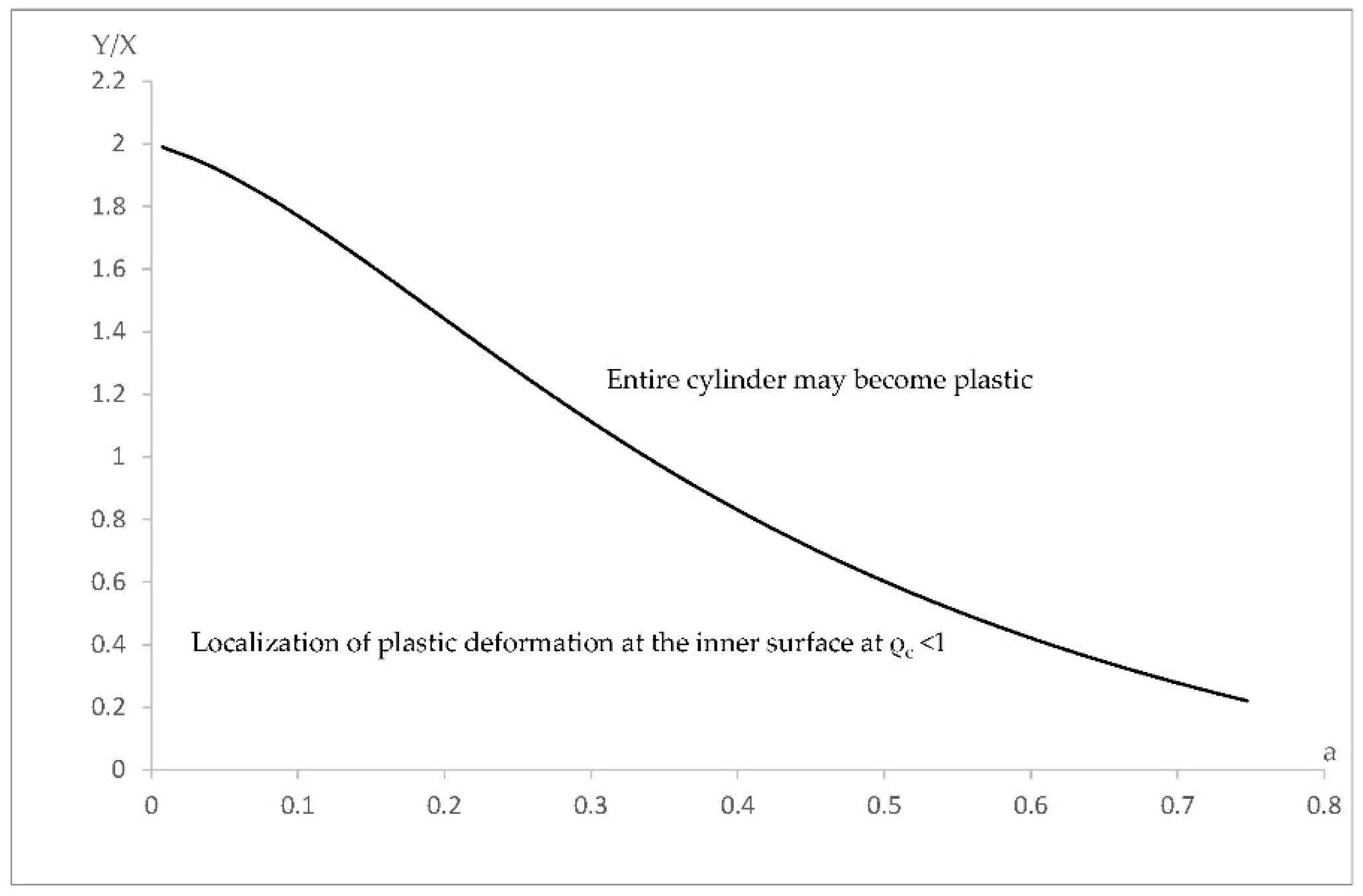
p 0 2 Q p p .
If p 0 = p p , then the localization of plastic deformation occurs at the inner radius of the cylinder, and the plastic region cannot propagate beyond the radius reached at this value of p 0 .
Consider the state of stress in the cylinder when the entire cylinder becomes plastic, and the localization of plastic deformation occurs at the inner radius of the cylinder simultaneously. The latter condition requires φ a = π / 2 . On the other hand, the stresses in Equation (20) should satisfy the boundary condition in Equation (2). It is reasonable to assume that at σ θ > 0 at ρ = 1 . Then, Equations (2) and (20) combine to give φ c = π . It is evident that ρ c = 1 . Substituting φ a = π / 2 , φ c = π , and ρ c = 1 into Equation (25) yields
ln a = 2 ln Q ( 1 + Q 2 ) Q π ( 1 + Q 2 ) .
Here, Q can be eliminated using its definition. Then, Equation (32) determines a relationship between a and Y / X corresponding to the state of stress in question. This relation is illustrated in Figure 1. If the point corresponding to a pair ( a , Y / X ) lies above the curve, then the entire disc becomes plastic before the localization of plastic deformation at the inner surface of the cylinder, and vice versa.
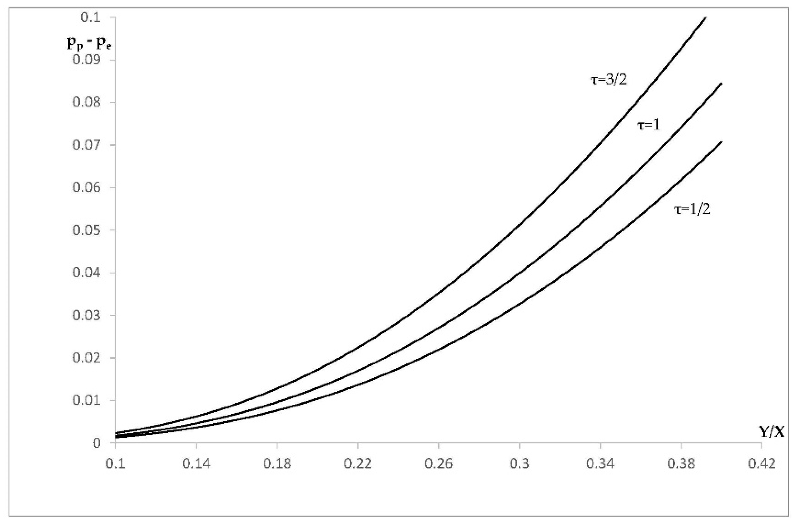
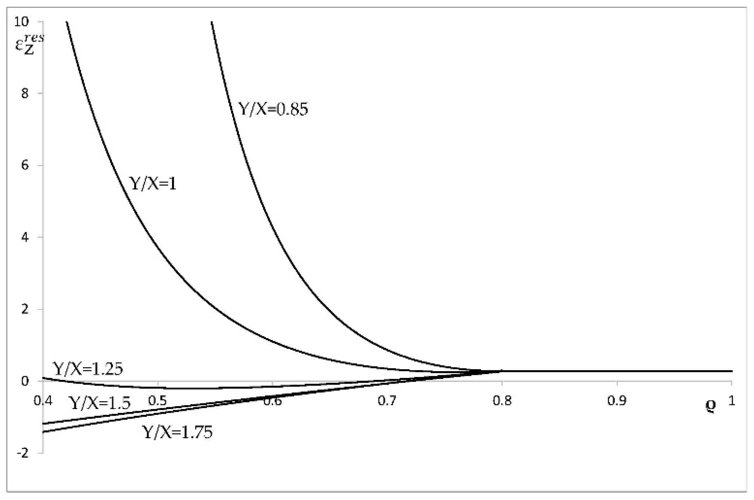
It is also of importance to consider the difference between p e and p p . It is seen from Equations (19) and (31) that p p is the function only of Y / X , whereas p e depends on Y / X , a, and τ . The variation of p p p e with Y / X at a = 0.4 for several values of τ is depicted in Figure 2. It is seen from this figure that the difference is rather small if the ratio Y / X is small enough. This means that the localization of plastic deformation at the inner surface of the cylinder occurs at the very beginning of plastic yielding.

5. Elastic/Plastic Strain Solution

The total strain is elastic in the region ρ c ρ 1 . Therefore, using Equation (12), the principal strains in this region are found from the generalized Hooke’s law in Equation (5) and the stress solution of Equation (26), as
ε r k = C 1 [ ( 1 + τ a r θ a r r ) ρ τ 1 + ( τ a r θ a r r 1 ) ρ τ 1 ] , ε θ k = C 1 [ ( a r θ a r r + τ a θ θ a r r ) ρ τ 1 + ( τ a θ θ a r r a r θ a r r ) ρ τ 1 ] , ε z k = C 1 [ ( a r z a r r + τ a θ z a r r ) ρ τ 1 + ( τ a θ z a r r a r z a r r ) ρ τ 1 ] .
Using Equation (12), the elastic portion of strain in the plastic region, a ρ ρ c , is determined from the generalized Hooke’s law (Equation (5)) and the stress solution in Equation (20), as
ε r e k = ( 2 + a r θ / a r r ) Q sin φ a r θ a r r cos φ , ε θ e k = ( 2 a r θ + a θ θ ) Q a r r sin φ a θ θ a r r cos φ , ε z e k = 2 a r z sin φ a r r Q a θ z a r r ( sin φ Q + cos φ ) .
Substituting Equation (20) into Equation (8) leads to
ξ r p = λ [ sin φ Q ( 1 4 X 2 Y 2 ) + cos φ ] , ξ θ p = 2 λ cos φ , ξ z p = λ [ ( 4 X 2 Y 2 1 ) sin φ Q + cos φ ] .
Eliminating λ between these equations gives
ξ r p ξ θ p = Q 2 ( 4 X 2 Y 2 1 ) tan φ 1 2 , ξ z p ξ θ p = Q 2 ( 4 X 2 Y 2 1 ) tan φ 1 2 .
In what follows, it is assumed that q φ a and
ξ r e = ε r e φ a , ξ θ e = ε θ e φ a , ξ z e = ε z e φ a , ξ r = ε r φ a , ξ θ e = ε θ φ a , ξ z e = ε z φ a .
Then, differentiating Equation (34) with respect to φ a yields
ξ r e k = [ ( 2 + a r θ / a r r ) Q cos φ + a r θ a r r sin φ ] φ φ a , ξ θ e k = [ ( 2 a r θ + a θ θ ) Q a r r cos φ + a θ θ a r r sin φ ] φ φ a , ξ z e k = [ 2 a r z cos φ a r r Q + a θ z a r r ( cos φ Q sin φ ) ] φ φ a .
Substituting Equation (9) differentiated with respect to φ a into Equation (11) and using Equation (12) leads to
ρ ξ θ ρ + ξ θ ξ r p ξ r e = 0 .
Moreover, using Equation (36),
ξ r p = [ Q 2 ( 4 X 2 Y 2 1 ) tan φ 1 2 ] ξ θ p = [ Q 2 ( 4 X 2 Y 2 1 ) tan φ 1 2 ] ( ξ θ ξ θ e )
Then, eliminating ξ r p in Equation (39) by means of Equation (40) yields
ρ ξ θ ρ + ξ θ 2 [ 3 Q ( 4 X 2 Y 2 1 ) tan φ ] + [ Q 2 ( 4 X 2 Y 2 1 ) tan φ 1 2 ] ξ θ e ξ r e = 0 .
Using Equation (21), differentiation with respect to ρ in Equation (41) can be replaced with differentiation with respect to φ . As a result,
ξ θ φ ( Q tan φ ) + ξ θ [ 3 Q ( 4 X 2 Y 2 1 ) tan φ ] + [ Q ( 4 X 2 Y 2 1 ) tan φ 1 ] ξ θ e 2 ξ r e = 0 .
It is seen from (38) that the expressions for ξ r e and ξ θ e involve the derivative φ / φ a . In general, this derivative can be found from Equation (24), which is the solution of Equation (21). However, it is more convenient to represent the solution of this equation satisfying the boundary condition Equation (22) as
ln ρ a = 2 φ a φ cos η ( Q cos η sin η ) d η
where η is a dummy variable of integration. Differentiating Equation (43) gives
2 cos φ ( Q cos φ sin φ ) d φ = 2 cos φ a ( Q cos φ a sin φ a ) d φ a + d ρ ρ .
It follows from this equation that
φ φ a = cos φ a ( Q cos φ sin φ ) cos φ ( Q cos φ a sin φ a ) .
Equations (38) and (44) combine to give
ξ r e k = [ ( 2 + a r θ / a r r ) Q cos φ + a r θ a r r sin φ ] ( Q tan φ ) ( Q tan φ a ) , ξ θ e k = [ ( 2 a r θ + a θ θ ) Q a r r cos φ + a θ θ a r r sin φ ] ( Q tan φ ) ( Q tan φ a ) , ξ z e k = [ 2 a r z cos φ a r r Q + a θ z a r r ( cos φ Q sin φ ) ] ( Q tan φ ) ( Q tan φ a ) .
Eliminating ξ r e and ξ θ e in Equation (42) by means of Equation (45) results in the following linear differential equation for ξ θ / k :
( ξ θ / k ) φ + ξ θ k Φ 1 ( φ ) + Φ 2 ( φ ) ( Q tan φ a ) = 0 , Φ 1 ( φ ) = [ 3 Q ( 4 X 2 Y 2 1 ) tan φ ] ( Q tan φ ) 1 ,
Φ 2 ( φ ) = [ a θ θ sin φ ( 2 a r θ + a θ θ ) Q cos φ ] [ Q ( 4 X 2 Y 2 1 ) tan φ 1 ] + 2 [ ( 2 a r r + a r θ ) Q cos φ a r θ sin φ ] .
The circumferential strain rate must be continuous across the elastic/plastic boundary. Therefore, the boundary condition to Equation (46) is
ξ θ k = ξ c k
for φ = φ c . Here, ξ c is the value of ξ θ on the elastic side of the elastic/plastic boundary. Differentiating the second equation in Equation (33) with respect to φ a , and then putting ρ = ρ c results in
ξ c k = d C 1 d φ a [ ( a r θ a r r + τ a θ θ a r r ) ρ c τ 1 + ( τ a θ θ a r r a r θ a r r ) ρ c τ 1 ] .
It is seen from this equation that it is necessary to find the derivative d C 1 / d φ a . It follows from Equation (43) that
ln ρ c a = 2 φ a φ c cos φ ( Q cos φ sin φ ) d φ .
Differentiating this equation and Equation (28) with respect to φ a yields
d φ c d φ a = ( Q tan φ c ) 2 [ d ρ c ρ c d φ a + 2 ( Q tan φ a ) ]
and
d φ c d φ a = 8 τ 2 ρ c 2 τ 1 sin 2 φ c Q ( ρ c 2 τ 1 ) 2 d ρ c d φ a ,
respectively. Solving Equations (50) and (51) for the derivatives d ρ c / d φ a and d φ c / d φ a gives
d ρ c d φ a = ( Q tan φ c ) ( Q tan φ a ) [ 8 τ 2 ρ c 2 τ 1 sin 2 φ c Q ( ρ c 2 τ 1 ) 2 ( Q tan φ c ) 2 ρ c ] 1 , d φ c d φ a = 8 τ 2 ρ c 2 τ 1 sin 2 φ c ( Q tan φ c ) Q ( ρ c 2 τ 1 ) 2 ( Q tan φ a ) [ 8 τ 2 ρ c 2 τ 1 sin 2 φ c Q ( ρ c 2 τ 1 ) 2 ( Q tan φ c ) 2 ρ c ] 1 .
The derivative d C 1 / d φ a is determined from the first equation in Equation (27) as
d C 1 d φ a = 2 sin φ c [ ( τ 1 ) ρ c τ 2 + ( τ + 1 ) ρ c τ 2 ] Q ( ρ c τ 1 ρ c τ 1 ) 2 d ρ c d φ a 2 cos φ c Q ( ρ c τ 1 ρ c τ 1 ) d φ c d φ a
In this equation, the derivatives d ρ c / d φ a and d φ c / d φ a can be eliminated by means of Equation (52). In the previous section, φ c and ρ c have been found as functions of φ a . Therefore, Equations (48) and (53) combine to supply ξ c / k as a function of φ a . Then, the solution of Equation (46), satisfying the boundary condition of Equation (47), can be solved numerically.
By definition, ξ θ = ε θ / φ a if ξ θ and ε θ are regarded as functions of φ a and ρ . However, the solution of Equation (46) provides ξ θ as a function of φ a and φ . In this case, ε θ φ a + ε θ φ φ φ a = ξ θ .
In this equation, the derivative φ / φ a can be eliminated by means of Equation (44). Then,
ε θ φ a + ε θ φ ( Q tan φ ) ( Q tan φ a ) = ξ θ .
Using a standard technique, it is possible to find that the equation of the characteristics is
d φ = ( Q tan φ ) ( Q tan φ a ) d φ a
and the relation along the characteristics is
d ( ε θ k ) = ξ θ k d φ a .
Equation (55) can be immediately integrated to give
Q ( φ a φ ) + ln ( Q cos φ sin φ Q cos φ a sin φ a ) = D
where D is a constant of integration. The boundary condition to Equation (56) is that ε θ / k = ε θ e / k at the elastic/plastic boundary. Here ε θ e is the circumferential strain on the elastic side of the elastic/plastic boundary. Using Equation (33), this boundary condition is represented as
ε θ k = C 1 [ ( a r θ a r r + τ a θ θ a r r ) ρ c τ 1 + ( τ a θ θ a r r a r θ a r r ) ρ c τ 1 ]
for ρ = ρ c (or φ = φ c ).
It is evident from Equation (57) that φ = φ a is a characteristic curve, and that D = 0 on this curve. Having ξ θ / k as a function of φ a at φ = φ a (or ρ = a ) from the solution of Equation (46), it is possible to integrate Equation (56) along the characteristic curve φ = φ a 
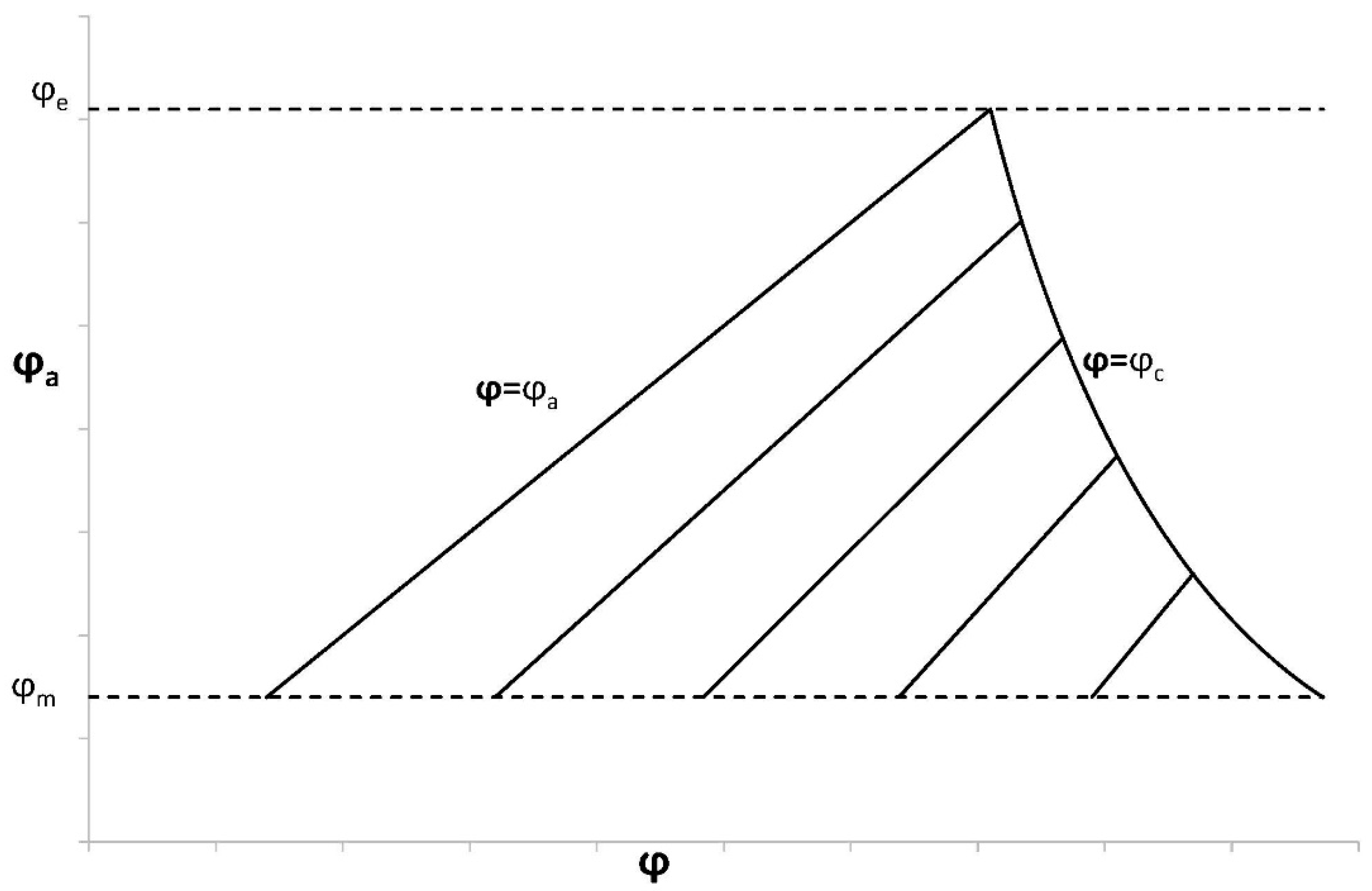
with the use of the boundary condition in Equation (58), to find the circumferential strain at the inner radius of the cylinder without solving Equation (54) for the entire plastic region. In order to illustrate the procedure for finding the strain solution in the entire plastic region, consider a schematic field of characteristics shown in Figure 3, where φ m is the value of φ a at the end of loading. Since φ c as a function of φ a is found from the solution of Equation (28), the curve φ = φ c is known. Choosing any pair ( φ a , φ ) on this curve, it is possible to find D from Equation (57). The corresponding characteristic curve follows from Equation (57) at this value of D if φ a varies in the range φ e φ a φ m . In particular, the value of φ at φ a = φ m is determined. This value of φ is denoted as φ M . The value of the circumferential strain at φ a = φ M and φ = φ M is found from the solution of Equation (56) satisfying the boundary condition of Equation (58). The plastic portion of this strain is immediate from Equations (9) and (34). Having found the distribution of ξ θ / k along the characteristic curve, it is possible to determine the distribution of ξ θ p / k using the equation ξ θ p / k = ξ θ / k ξ θ e / k and Equation (45). Then, Equation (36) supplies the distribution of ξ r p / k and ξ z p / k .
By analogy to Equation (54), it is possible to get
ε r p φ a + ε z p φ ( Q tan φ ) ( Q tan φ a ) = ξ θ p , ε z p φ a + ε z p φ ( Q tan φ ) ( Q tan φ a ) = ξ z p .
These equations can be integrated in the same manner as Equation (54). In particular, Equation (57) is the equation of characteristic curves. The boundary conditions are
ε r p = ε z p = 0
for ρ = ρ c (or φ = φ c ). Once the values of ε r p and ε z p at φ a = φ m and φ = φ M have been found, the total strains are immediate from Equations (9) and (34). The strain solution described supplies the variation of strain components with φ at a given value of φ a . In order to find the radial distributions, it is necessary to use Equation (24).

6. Unloading

It is assumed that the process of unloading is purely elastic. This assumption should be verified a posteriori. The general elastic solution of Equation (13), in which the stress components are replaced with their increments, is valid in the entire cylinder. Then,
Δ σ r X = C 3 ρ τ 1 + C 4 ρ τ 1 , Δ σ θ X = τ ( C 3 ρ τ 1 C 4 ρ τ 1 )
where C 3 and C 4 are new constants of integration. These constants are found from the boundary conditions of Equations (3) and (4). As a result,
C 3 = C 4 = p m ( a τ 1 a τ 1 ) .
Here, Equation (12) has been taken into account. Substituting Equation (62) into (61) supplies the radial distribution of Δ σ r and Δ σ θ in the form
Δ σ r X = p m ( a τ 1 a τ 1 ) ( ρ τ 1 ρ τ 1 ) , Δ σ θ X = τ p m ( a τ 1 a τ 1 ) ( ρ τ 1 + ρ τ 1 ) .
The variation of the residual stresses with ρ is found as
σ r r e s = σ r + Δ σ r   and   σ θ r e s = σ θ + Δ σ θ .
It is understood here that σ r and σ θ are known from the stress solution given in Section 4, at p 0 = p m . The process of unloading is purely elastic if the yield criterion is not violated in the entire cylinder. Using Equation (6), this condition can be represented as
( σ θ r e s X ) 2 ( σ θ r e s X ) ( σ r r e s X ) + ( σ r r e s X ) 2 X 2 Y 2 1
in the range a ρ 1 . The radial distribution of the strain increments is determined from the generalized Hooke’s law in Equations (5) and (62), as
Δ ε r e k = p m ( a τ 1 a τ 1 ) [ ( 1 + τ a r θ a r r ) ρ τ 1 ρ τ 1 ( 1 τ a r θ a r r ) ] , Δ ε θ e k = p m ( a τ 1 a τ 1 ) [ ( a r θ a r r + τ a θ θ a r r ) ρ τ 1 ( a r θ a r r τ a θ θ a r r ) ρ τ 1 ] , Δ ε z e k = p m ( a τ 1 a τ 1 ) [ ( a r z a r r + τ a θ z a r r ) ρ τ 1 ( a r z a r r τ a θ z a r r ) ρ τ 1 ] .
The variation of the residual strains with ρ is found as
ε r r e s = ε r + Δ ε r ,   ε θ r e s = ε θ + Δ ε θ   and   ε z r e s = ε z + Δ ε z .
It is understood here that ε r , ε θ , and ε z are known from the strain solution given in Section 5 at p 0 = p m .

7. Numerical Example

This section illustrates the effect of plastic anisotropy on the distribution of stress and strain in an a = 0.4 cylinder, assuming that the elastic properties are isotropic. In particular, it is assumed that Poisson’s ratio is equal to 0.3 (i.e., a r θ = 0.3 ). The value of k is immaterial, because all strains are proportional to k. The solution given in Section 4 has been used to calculate the radial distribution of the radial and circumferential stress corresponding to ρ c = 0.8 . It is seen from Figure 1 that the solution without the localization of plastic deformation at the inner radius of the cylinder exists only if Y / X > 0.8 . Therefore, the stress solution has been found at Y / X = 0.85 , Y / X = 1 (isotropic material), Y / X = 1.25 , and Y / X = 1.5 . This solution is illustrated in Figure 4 (radial stress) and Figure 5 (circumferential stress). The associate strain solution has been found using the approach described in Section 5. This strain solution is illustrated in Figure 6 (total radial strain), Figure 7 (total circumferential strain), and Figure 8 (total axial strain). It can be seen from these figures that the effect of the ratio Y / X on the distribution of the strains is very significant in the range Y / X < 1.25 
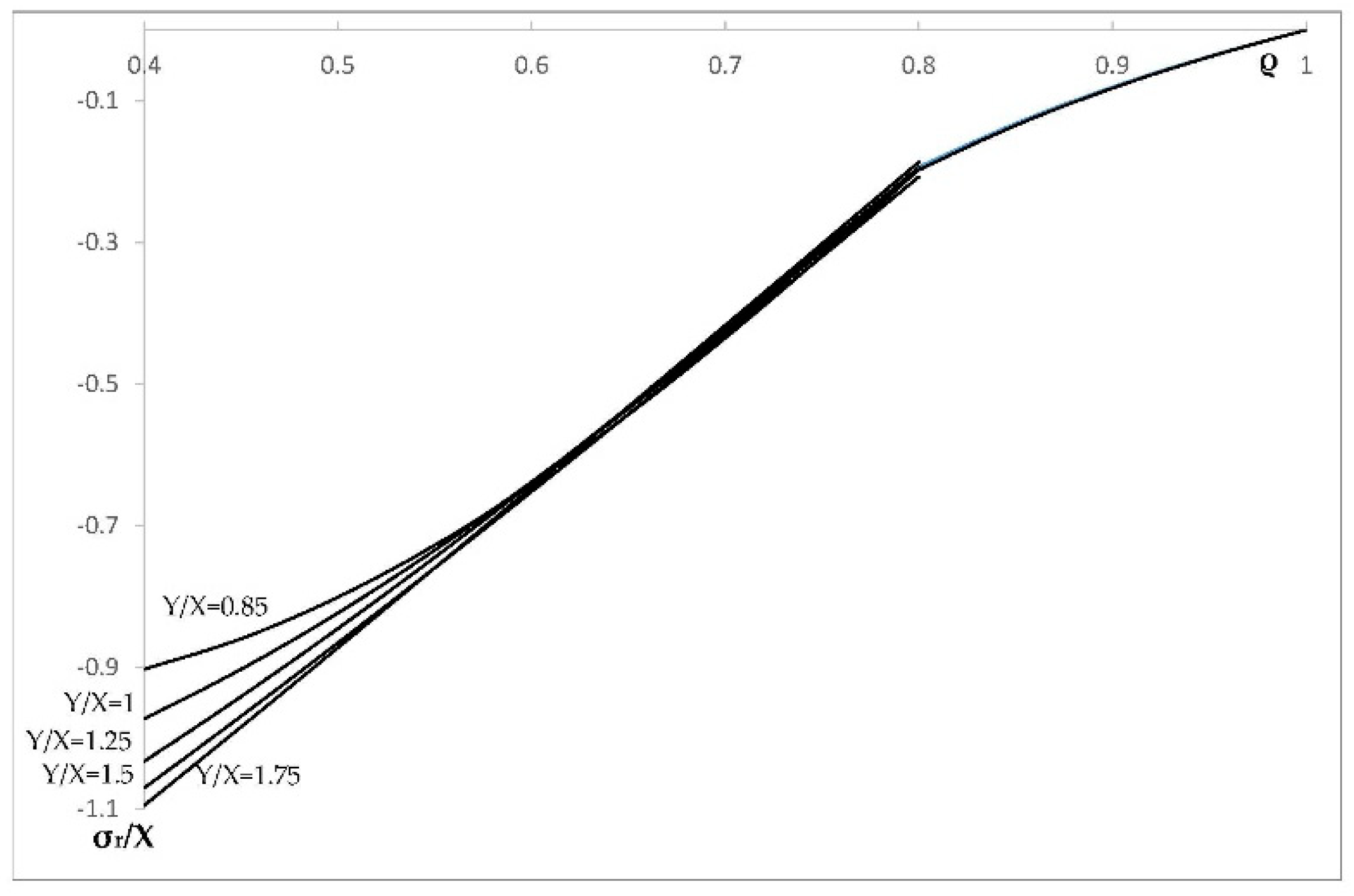
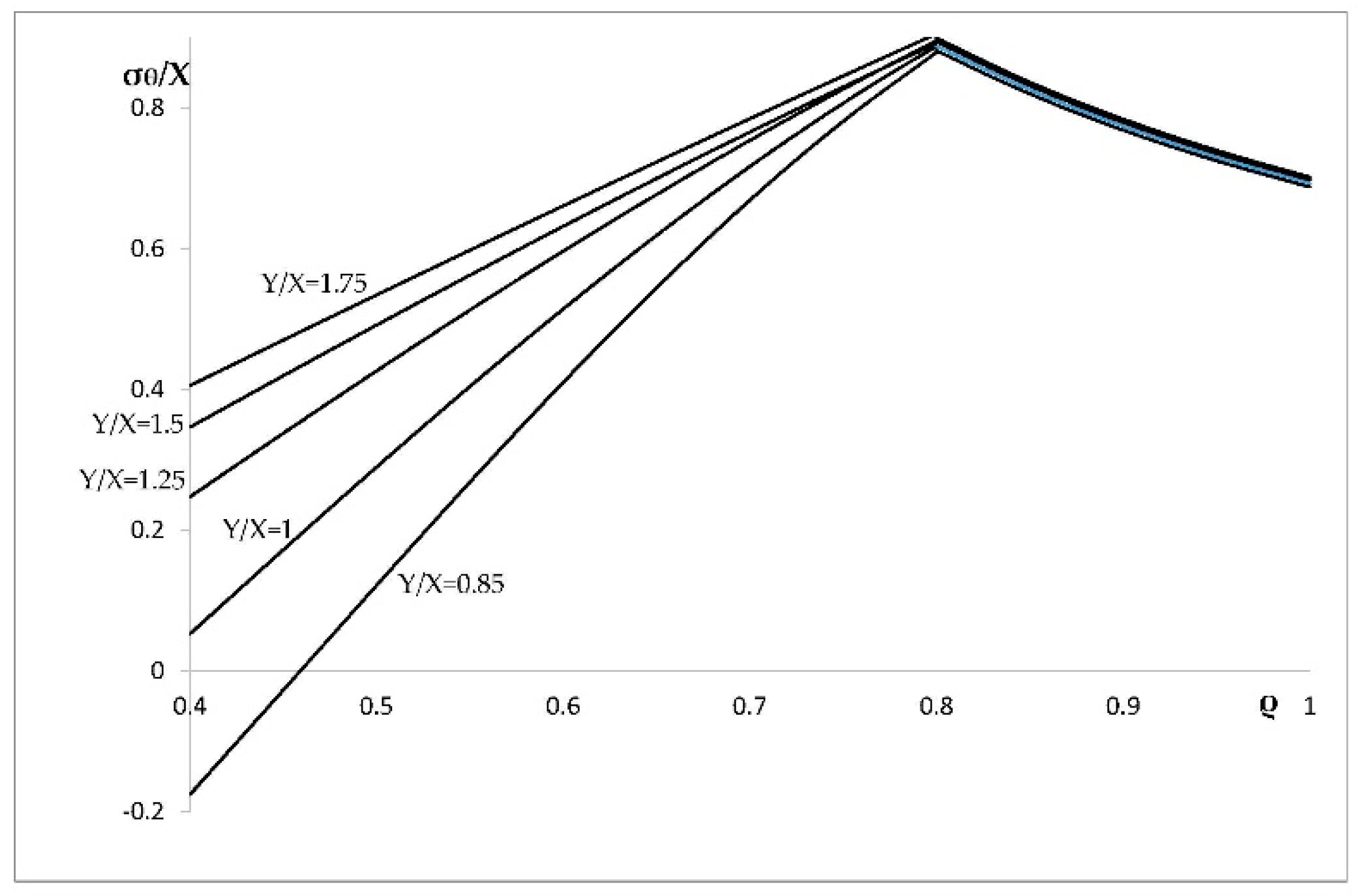
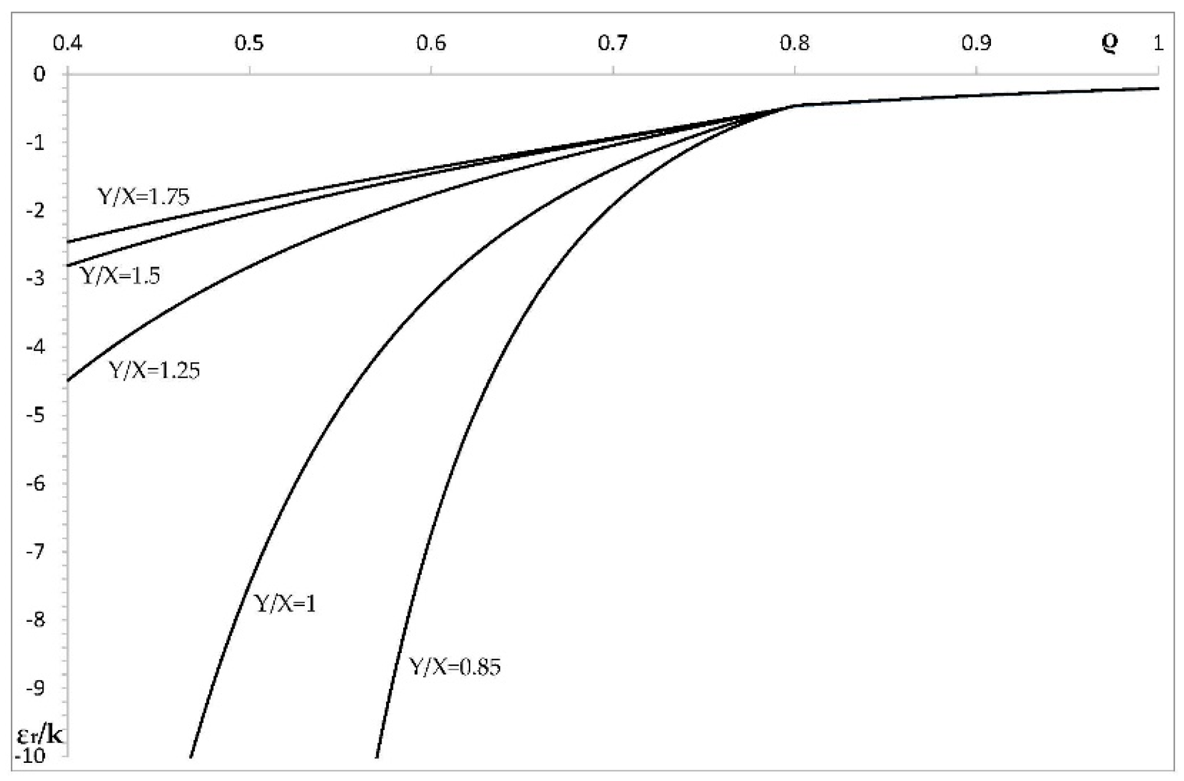
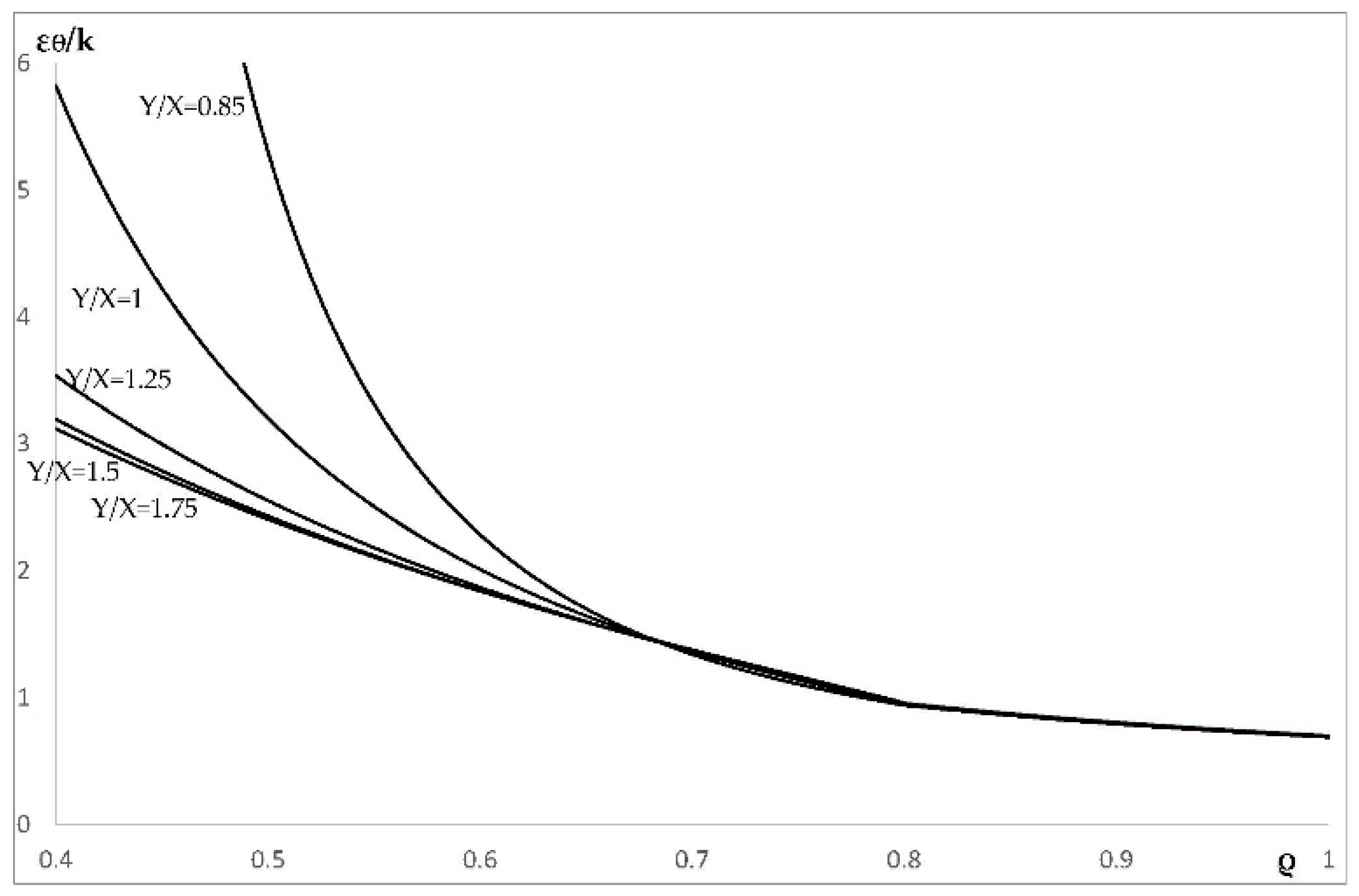
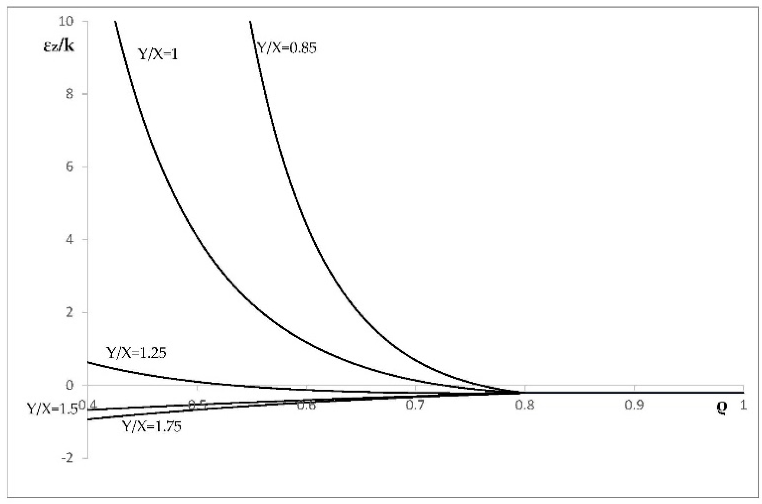
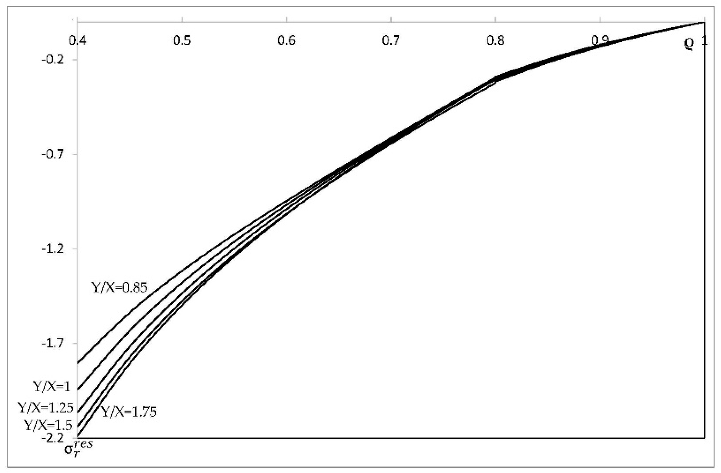
. In this range, the magnitude of strains is very large in the vicinity of the inner surface of the cylinder, which indicates the tendency towards the localization of plastic deformation. Since the solution found is for small strains, it is necessary to verify for each combination of material and geometric parameters that the assumption of small strain is acceptable. The distribution of the residual stresses has been determined using the stress distributions depicted in Figure 4 and Figure 5, in conjunction with the solution provided in 
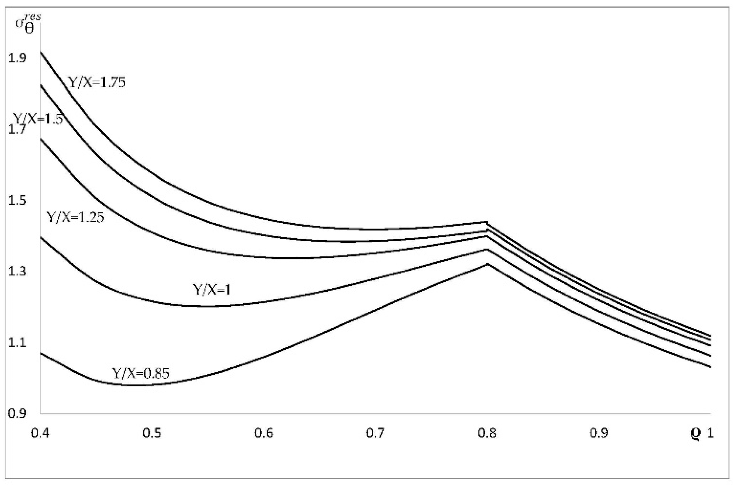
Section 6. This solution is illustrated in Figure 9 (residual radial stress) and 
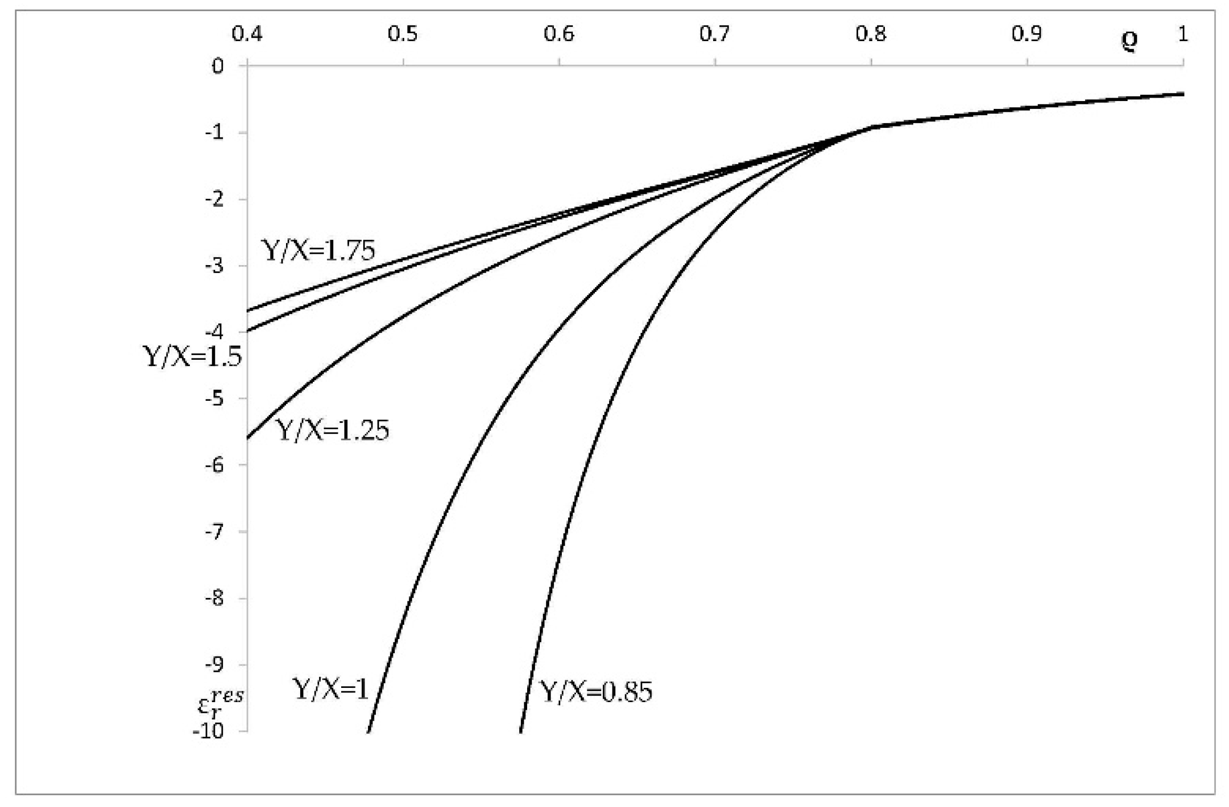
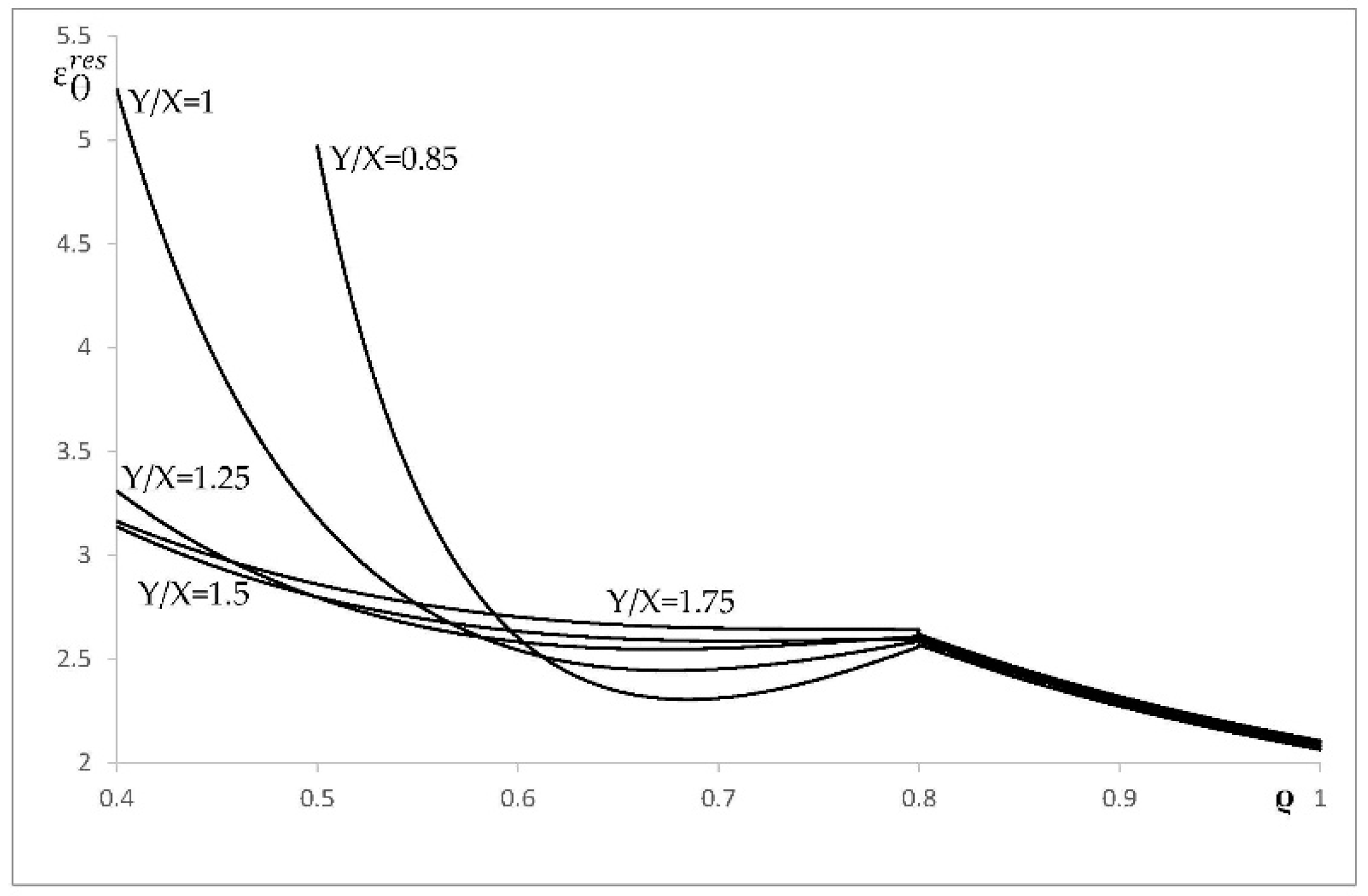
Figure 10 (residual circumferential stress). The associate strain solution has been found using the approach described in Section 6. This solution for residual strains is illustrated in Figure 11 (residual radial strain), Figure 12 (residual circumferential strain), and Figure 13 (residual axial strain). As in the case of the strain distribution at the end of loading, it is seen from these figures that the solution is very sensitive to the value of Y / X in the range Y / X < 1.25 . The residual circumferential stress is of special significance for autofrettage. It is seen from Figure 10 that the magnitude of this stress at the inner surface of the cylinder is significantly affected by plastic anisotropy.

8. Conclusions

A new theoretical solution for the distribution of residual stresses and strains in an open-ended, thick-walled cylinder subjected to internal pressure followed by unloading has been proposed. A distinguished feature of this solution is that the cylinder is initially anisotropic. In particular, the paper is concentrated on a common type of anisotropy: polar orthotropy of elastic and plastic properties. The elastic response of the cylinder is controlled by the generalized Hooke’s law, and the plastic response by the Tsai–Hill yield criterion and its associated flow rule. The flow theory of plasticity is employed. It has been shown that using the strain rate compatibility equation facilitates the solution. In particular, numerical techniques are only necessary to solve the linear differential Equation (46), and to evaluate ordinary integrals along characteristic curves.
The solution found can be directly used for the analysis and design of the process of autofrettage. It is worthy of note that in this case, there is no need to construct the field of strain in the entire cylinder, which is the most difficult part of the numerical solution. It follows from Equation (57) that φ = φ a is a characteristic curve, and this curve corresponds to the inner surface of the cylinder. The circumferential strain along this curve can be immediately found from Equation (56). Therefore, the radius of the cylinder after unloading is determined. The circumferential stress at the inner radius of the cylinder at the end of loading follows from Equation (20) at φ = φ a . Then, the corresponding residual stress is immediate from Equations (61), (62), and (64).
An illustrative example is given in Section 7. In this case, it is assumed that the elastic properties are isotropic. As a result, the effect of the ratio Y / X on the distribution of stresses and strains has been revealed. This effect is especially significant in the range Y / X < 1.25 (Figure 5, Figure 6, Figure 7, Figure 8 and Figure 10, Figure 11, Figure 12, Figure 13). An exception is the distribution of the radial stress at the end of loading and after unloading. (Figure 4 and Figure 9). This is because the boundary conditions on σ r and Δ σ r , from Equations (2) and (94), dictate that this stress vanishes at the inner radius of the cylinder.

Author Contributions

All three authors participated in the research and in the writing of this paper.

Funding

S.A. acknowledges support from the Russian Foundation for Basic Research (Project 16-08-00469).

Acknowledgments

This work was initiated while M.R. was a visiting researcher at Beihang University, Beijing, China. The publication has been prepared with the support of the “RUDN University Program 5-100”.

Conflicts of Interest

The authors declare no conflict of interest.

References

  1. Hill, R.; Lee, E.H.; Tupper, S.J. The theory of combined plastic and elastic deformation with particular reference to a thick tube under internal pressure. Proc. Roy. Soc. London. Series A Math. Phys. Sci. 1947, 191, 278–303. [Google Scholar] [Green Version]
  2. Hill, R. The Mathematical Theory of Plasticity; Clarendon Press: Oxford, UK, 1950. [Google Scholar]
  3. Thomas, D.G.B. The autofrettage of thick tubes with free ends. J. Mech. Phys. Solids 1953, 1, 124–133. [Google Scholar] [CrossRef]
  4. Rees, D.W.A. Autofrettage theory and fatigue life of open-ended cylinders. J. Strain Anal. 1990, 25, 109–121. [Google Scholar] [CrossRef]
  5. Gao, X. An exact elasto-plastic solution for an open-ended thick-walled cylinder of a strain-hardening material. Int. J. Press. Vessels Pip. 1992, 52, 129–144. [Google Scholar] [CrossRef]
  6. Hosseinian, E.; Farrahi, G.H.; Movahhedy, M.R. An analytical framework for the solution of autofrettaged tubes under constant axial strain condition. J. Press. Vessel Techn. 2009, 131, 1–8. [Google Scholar] [CrossRef]
  7. Molaie, M.; Darijani, H.; Bahreman, M.; Hosseini, S.M. Autofrettage of nonlinear strain-hardening cylinders using the proposed analytical solution for stresses. Int. J. Mech. Sci. 2018, 141, 450–460. [Google Scholar] [CrossRef]
  8. Rees, D.W.A. A theory for swaging of discs and lugs. Meccanica 2011, 46, 1213–1237. [Google Scholar] [CrossRef]
  9. Gao, X.-L.; Wen, J.-F.; Xuan, F.-Z.; Tu, S.-T. Autofrettage and shakedown analyses of an internally pressurized thick-walled cylinder based on strain gradient plasticity solutions. J. Appl. Mech. 2015, 82, 1–12. [Google Scholar] [CrossRef]
  10. Chen, P.C.T. The Bauschinger and Hardening effect on residual stresses in an autofrettaged thick-walled cylinder. Press. Vessel Techn. 1986, 108, 108–112. [Google Scholar] [CrossRef]
  11. Livieri, P.; Lazzarin, P. Autofrettaged cylindrical vessels and bauschinger effect: An analytical frame for evaluating residual stress distributions. J. Press. Vessel Techn. 2002, 124, 38–46. [Google Scholar] [CrossRef]
  12. Parker, A.P.; Gibson, M.C.; Hameed, A.; Troiano, E. Material modeling for autofrettage stress analysis including the “single effective material”. J. Press. Vessel Techn. 2012, 134, 1–7. [Google Scholar] [CrossRef]
  13. Gibson, M.C.; Parker, A.P.; Hameed, A.; Hetherington, J.G. Implementing realistic, nonlinear, material stress–strain behavior in ANSYS for the autofrettage of thick-walled cylinders. J. Press. Vessel Techn. 2012, 134, 1–7. [Google Scholar] [CrossRef]
  14. Perl, M.; Perry, J. The beneficial influence of bauschinger effect mitigation on the barrel’s safe maximum pressure. J. Press. Vessel Techn. 2013, 135, 1–5. [Google Scholar] [CrossRef]
  15. Farrahi, G.H.; Voyiadjis, G.Z.; Hoseini, S.H.; Hosseinian, E. Residual stress analysis of the autofrettaged thick-walled tube using nonlinear kinematic hardening. J. Press. Vessel Techn. 2013, 135, 1–8. [Google Scholar] [CrossRef]
  16. Haghpanah Jahromi, B.; Farrahi, G.H.; Maleki, M.; Nayeb-Hashemia, H.; Vaziri, A. Residual stresses in autofrettaged vessel made of functionally graded material. Eng. Struct. 2009, 31, 2930–2935. [Google Scholar] [CrossRef]
  17. Jahed, H.; Farshi, B.; Karimi, M. Optimum autofrettage and shrink-fit combination in multi-layer cylinders. J. Press. Vessel Techn. 2006, 128, 196–200. [Google Scholar] [CrossRef]
  18. Lee, E.-Y.; Lee, Y.-S.; Yang, Q.-M.; Kim, J.-H.; Cha, K.-U.; Hong, S.-K. Autofrettage process analysis of a compound cylinder based on the elastic-perfectly plastic and strain hardening stress-strain curve. J. Mech. Sci. Techn. 2009, 23, 3153–3160. [Google Scholar] [CrossRef]
  19. Gexia, Y.; Hongzhao, L. An analytical solution of residual stresses for shrink-fit two-layer cylinders after autofrettage based on actual material behavior. J. Press. Vessel Techn. 2012, 134, 1–8. [Google Scholar] [CrossRef]
  20. Benghalia, G.; Wood, J. Material and residual stress considerations associated with the autofrettage of weld clad components. Int. J. Press. Vessels Pip. 2016, 139–140, 146–158. [Google Scholar] [CrossRef]
  21. Abdelsalam, O.R.; Sedaghati, R. Design optimization of compound cylinders subjected to autofrettage and shrink-fitting processes. J. Press. Vessel Techn. 2013, 135, 1–11. [Google Scholar] [CrossRef]
  22. Hu, C.; Yang, F.; Zhao, Z.; Zeng, F. An alternative design method for the double-layer combined die using autofrettage theory. Mech. Sci. 2017, 8, 267–276. [Google Scholar] [CrossRef] [Green Version]
  23. Seifi, R. Maximizing working pressure of autofrettaged three layer compound cylinders with considering Bauschinger effect and reverse yielding. Meccanica 2018, 53, 2485–2501. [Google Scholar] [CrossRef]
  24. Hamilton, N.R.; Wood, J.; Easton, D.; Olsson Robbie, M.B.; Zhang, Y.; Galloway, A. Thermal autofrettage of dissimilar material brazed joints. Mater. Des. 2015, 67, 405–412. [Google Scholar] [CrossRef] [Green Version]
  25. Kamal, S.M.; Dixit, U.S. Feasibility study of thermal autofrettage of thick-walled cylinders. J. Press. Vessel Techn. 2015, 137, 1–18. [Google Scholar] [CrossRef]
  26. Kamal, S.M.; Borsaikia, A.C.; Dixit, U.S. Experimental assessment of residual stresses induced by the thermal autofrettage of thick-walled cylinders. J. Strain Anal. 2016, 51, 144–160. [Google Scholar] [CrossRef]
  27. Shufen, R.; Dixit, U.S. An analysis of thermal autofrettage process with heat treatment. Int. J. Mech. Sci. 2018, 144, 134–145. [Google Scholar] [CrossRef]
  28. Zare, H.R.; Darijani, H. A novel autofrettage method for strengthening and design of thick-walled cylinders. Mater. Des. 2016, 105, 366–374. [Google Scholar] [CrossRef]
  29. Kamal, S.M. Analysis of residual stress in the rotational autofrettage of thick-walled disks. J. Press. Vessel Techn. 2018, 140, 1–10. [Google Scholar] [CrossRef]
  30. Shufen, R.; Dixit, U.S. A review of theoretical and experimental research on various autofrettage processes. ASME J. Press. Vessel Technol. 2018, 140, 050802. [Google Scholar] [CrossRef]
  31. Alexandrov, S.; Chung, K.-H.; Chung, K. Effect of plastic anisotropy of weld on limit load of undermatched middle cracked tension specimens. Fat. Fract. Engng. Mater. Struct 2007, 30, 333–341. [Google Scholar] [CrossRef]
  32. Alexandrov, S.; Mustafa, Y. Influence of plastic anisotropy on the limit load of highly under-matched scarf joints with a crack subject to tension. Eng. Fract. Mech. 2014, 131, 616–626. [Google Scholar] [CrossRef]
  33. Prime, M.B. Amplified effect of mild plastic anisotropy on residual stress and strain anisotropy. Int. J. Solids Struct. 2017, 118, 70–77. [Google Scholar] [CrossRef]
  34. Alexandrova, N.; Alexandrov, S. Elastic-plastic stress distribution in a plastically anisotropic rotating disk. Trans. ASME J. Appl. Mech. 2004, 71, 427–429. [Google Scholar] [CrossRef]
  35. Alexandrova, N.; Vila Real, P.M.M. Effect of plastic anisotropy on stress-strain field in thin rotating disks. Thin-Walled Struct. 2006, 44, 897–903. [Google Scholar] [CrossRef]
  36. Peng, X.-L.; Li, X.-F. Elastic analysis of rotating functionally graded polar orthotropic disks. Int. J. Mech. Sci. 2012, 60, 84–91. [Google Scholar] [CrossRef]
  37. Essa, S.; Argeso, H. Elastic analysis of variable profile and polar orthotropic FGM rotating disks for a variation function with three parameters. Acta Mech. 2017, 228, 3877–3899. [Google Scholar] [CrossRef]
  38. Jeong, W.; Alexandrov, S.; Lang, L. Effect of plastic anisotropy on the distribution of residual stresses and strains in rotating annular disks. Symmetry 2018, 10, 420. [Google Scholar] [CrossRef]
  39. Yildirim, V. Numerical/analytical solutions to the elastic response of arbitrarily functionally graded polar orthotropic rotating discs. J. Brazilian Soc. Mech. Sci. Eng. 2018, 40, 320. [Google Scholar] [CrossRef]
  40. Leu, S.-Y.; Hsu, H.-C. Exact solutions for plastic responses of orthotropic strain-hardening rotating hollow cylinders. Int. J. Mech. Sci. 2010, 52, 1579–1587. [Google Scholar] [CrossRef]
  41. Abd-Alla, A.M.; Mahmoud, S.R.; AL-Shehri, N.A. Effect of the rotation on a non-homogeneous infinite cylinder of orthotropic material. Appl. Math. Comp. 2011, 217, 8914–8922. [Google Scholar] [CrossRef]
  42. Lubarda, V.A. On Pressurized curvilinearly orthotropic circular disk, cylinder and sphere made of radially nonuniform material. J. Elast. 2012, 109, 103–133. [Google Scholar] [CrossRef]
  43. Croccolo, D.; De Agostinis, M. Analytical solution of stress and strain distributions in press fitted orthotropic cylinders. Int. J. Mech. Sci. 2013, 71, 21–29. [Google Scholar] [CrossRef]
  44. Shahani, A.R.; Torki, H.S. Determination of the thermal stress wave propagation in orthotropic hollow cylinder based on classical theory of thermoelasticity. Cont. Mech. Thermodyn. 2018, 30, 509–527. [Google Scholar] [CrossRef]
  45. Callioglu, H.; Topcu, M.; Tarakcılar, A.R. Elastic–plastic stress analysis of an orthotropic rotating disc. Int. J. Mech. Sci. 2006, 48, 985–990. [Google Scholar] [CrossRef]
  46. Tarfaoui, M.; Nachtane, M.; Khadimallah, H.; Saifaoui, D. Simulation of mechanical behavior and damage of a large composite wind turbine blade under critical loads. Appl. Compos. Mater. 2018, 25, 237–254. [Google Scholar] [CrossRef]
  47. Quadrino, A.; Penna, R.; Feo, L.; Nicola Nistico, N. Mechanical characterization of pultruded elements: Fiber orientation influence vs web-flange junction local problem. Exp. Numer. Tests Compos. Part B 2018, 142, 68–84. [Google Scholar] [CrossRef]
  48. Morgado, T.; Silvestre, N.; Correia, J.R. Simulation of fire resistance behaviour of pultruded GFRP beams —Part II: Stress analysis and failure criteria. Comp. Struct. 2018, 188, 519–530. [Google Scholar] [CrossRef]
  49. Zhou, Y.; Duan, M.; Ma, J.; Sun, G. Theoretical analysis of reinforcement layers in bonded flexible marine hose under internal pressure. Eng. Struct. 2018, 168, 384–398. [Google Scholar] [CrossRef]
Figure 1. Geometric interpretation of two different mechanisms of plastic collapse (localization of plastic deformation at the inner radius of the cylinder and occurrence of the plastic region over the entire disc).
Symmetry 11 00280 g001
Figure 2. Effect of constitutive parameters on the magnitude of pressure at which plastic deformation is localized at the inner radius of the cylinder.
Symmetry 11 00280 g002
Figure 3. A schematic diagram showing the field of characteristics.
Symmetry 11 00280 g003
Figure 4. Variation of the radial stress with ρ in an a = 0.4 cylinder at several values of Y/X.
Symmetry 11 00280 g004
Figure 5. Variation of the circumferential stress with ρ in an a = 0.4 cylinder at several values of Y/X.
Symmetry 11 00280 g005
Figure 6. Variation of the total radial strain with ρ in an a = 0.4 cylinder at several values of Y/X.
Symmetry 11 00280 g006
Figure 7. Variation of the total circumferential strain with ρ in an a = 0.4 cylinder at several values of Y/X.
Symmetry 11 00280 g007
Figure 8. Variation of the total axial strain with ρ in an a = 0.4 cylinder at several values of Y/X.
Symmetry 11 00280 g008
Figure 9. Variation of the residual radial stress with ρ in an a = 0.4 cylinder at several values of Y/X.
Symmetry 11 00280 g009
Figure 10. Variation of the residual circumferential stress with ρ in an a = 0.4 cylinder at several values of Y/X.
Symmetry 11 00280 g010
Figure 11. Variation of the residual radial strain with ρ in an a = 0.4 cylinder at several values of Y/X.
Symmetry 11 00280 g011
Figure 12. Variation of the residual circumferential strain with ρ in an a = 0.4 cylinder at several values of Y/X.
Symmetry 11 00280 g012
Figure 13. Variation of the residual axial strain with ρ in an a = 0.4 cylinder at several values of Y/X.
Symmetry 11 00280 g013

