The Existence of Symmetric Positive Solutions of Fourth-Order Elastic Beam Equations

Department of Mathematics, Firat University, Elazığ 23100, Turkey
Symmetry 2019, 11(1), 121; https://doi.org/10.3390/sym11010121
Submission received: 10 December 2018
/
Revised: 10 January 2019
/
Accepted: 14 January 2019
/
Published: 20 January 2019
(This article belongs to the Special Issue Mathematical Physics and Symmetry)
Abstract
:In this study, we consider the eigenvalue problems of fourth-order elastic beam equations. By using Avery and Peterson’s fixed point theory, we prove the existence of symmetric positive solutions for four-point boundary value problem (BVP). After this, we show that there is at least one positive solution by applying the fixed point theorem of Guo-Krasnosel’skii.
1. Introduction
Consider the problem of the fourth-order four-point boundary value as given below. We will examine the existence of symmetric positive solutions for the following problem:
which defines the corruptions of an elastic beam with two stable endpoints, where → [0,∞) is continuous; y: (0, 1) → [0,∞) is symmetric on (0, 1) and possibly singular at and ; is called an eigenvalue and nontrivial solution as that λ is called an eigenfunction, with ; μ, α, γ and β are nonnegative constants; 0 ≤ 1 ≤ 2 ≤ 1 and is symmetric on [0, 1] for all u ∈ [0,∞), , for each ∈ [0,1] × [0,∞).
Fourth-order ordinary differential equations have important applications in engineering and physical sciences as they form the models related to bending or deformation of elastic beams. These problems, especially used in material mechanics, define the deformation of an elastic beam with two fixed endpoints. Building beams in buildings and bridge construction requires serious calculations to ensure the safety of the structure. As part of these calculations, it is important to evaluate the maximum deviations in the beams. The main objective is to provide a solution to the problem that the beam can safely support the intended load. Calculations often require complex and difficult operations. At this stage, different techniques in numerical integration and applied mathematics are applied.
Equation (1) is called the beam equation and is examined under different boundary conditions. Two or more point boundary value problems for these equations have attracted a significant amount of attention. Two-point boundary value problems have been studied extensively. Multi-point boundary value problems have also started to be examined in the literature. Many authors have investigated the beam equation under various boundary conditions and with different approaches. These studies include Tymoshenko’s study on elasticity [1], Soedel’s study on the deformation of the structure on monograms [2] and Dulácska study on the effects of [3] soil settlement.
Adequate conditions for the presence and absence of positive solutions for three-point boundary value problems were established by Graef et al. [4]. Siddiqi and Ghazala [5] determined the solution of the system of fourth-order boundary value problems using the non-cubic non-polynomial spline method. Ghazala and Hamood [6] used the fourth-degree solution to solve the reproducing kernel method (RKM) discrete boundary value problem. In the periodic beam equation examined with nonlinear boundary conditions, they used the Rayleigh–Ritz approach method. Avery and Peterson fixed point theorem, Iteration method and Leray–Schauder theorem have been used to solve these problems (See Gupta [7], Feng and Webb [8], Ma [9]).
In reference [9], Ma considered the fourth-order boundary problem with the two-point boundary conditions as follows:
Zhong and Chen [10] investigated the fourth-order nonlinear differential equation as follows:
with the ensuing four-point boundary value condition:
where 1234 are positive constants; and 12 12
In addition, Chen et al. [11] studied the following problem:
where ; μ is a positive constant, with (μ < 1); and , for any . In fact, Agarwal [12], Cabada [13] as well as De Coster and Sanchez [14] applied the upper and lower solution method for the fourth-order equation under Lidstone boundary conditions or other conditions:
In the case where is nonlinear, it obtains an infinite number of solutions under symmetrical conditions for λ = 1 and μ = 0.
In reference [15], they proved that the boundary value problem has at least one positive solution in the superlinear case, i.e., max 0 = 0 and min ∞ = ∞ or in the sublinear case, i.e., min 0 = ∞ and max ∞ = 0. These values can be as low as min 0 = max 0 = max ∞ = min ∞. The different studies examining this include those by Liu [16], Sun [17], Han [18], Wei and Pang [19], Zhong et al. [10] and Yao [20]. On the other hand, Adomian decomposition method was used to solve linear and nonlinear ordinary differential equations by Biazar and Shafiof [21] and Mestrovic [22]. This method provides the solution in a fast convergent series with computable terms. However, in order to solve boundary value problems using Adomian decomposition method (ADM), some unknown parameters must be determined and therefore, nonlinear algebraic equations must be solved. Geng and Cui [23] developed a method for solving nonlinear quadratic two-point BVP with the combination of ADM and RKM. Further detail can be found in studies of fourth-order boundary value problems [23,24,25,26,27,28,29,30,31].
In this article, our problem relates to the classical bending theory of flexible elastic beams on a nonlinear basis. Here, non-linear represents the force exerted on the elastic beam. We can use the expanding method to solve fourth-order four-point BVP, which was developed by Geng and Cui [23]. In our study, we have considered the following two problems: the first one can have a value as low as max 0 = max ∞ = 0 or min ∞ = min 0 = ∞. It can be as low as min 0 = max 0= max ∞ = min ∞ ∈ {0,∞}. In the conventional bending theory, the distortion of a flexible beam at both endpoints is given in Figure 1. Based on the theory, the in-plane displacement status in the x direction of the two parts can be determined. is used to represent the shear force along the beam. The shear force is used to calculate the shear stress on the cross-section of the beam. The maximum shear stress occurs at the neutral axis of the beam. This is the case of the superlinear problem.
The aim of this present study is to establish sufficient conditions for fourth-order nonlinear (1) and (2) problems with four-point boundary value conditions of min 0 = max 0= max ∞ = min ∞ ∈ {0,∞}, or max 0, max ∞, min 0, min ∞ ∈ {0, ∞} and to prove that the boundary value problem has at least one positive symmetric solution in the superlinear state. In contrast to the other studies, the Krasnosel‘skii [15] method was used and the results were shown in the last section and an example was given.
2. Preliminaries and Lemmas
Definition 1
([19]). is a real Banach space that takes a shut convex set , which is non-empty. This is defined as a contour of in the following two conditional cases:
- (1)
- implies
- (2)
- implies
Definition 2
([19]). If an operator is continuous, it is constantly constrained and the maps are set in restricted clusters.
Definition 3
([19]). Let be a cone on in Banach space. The function is said to be concave on if is continuous and:
for all and .
Definition 4
([17]). If the function is symmetric.
Definition 5
[17]). If [0, 1] is also positive and symmetric and corresponds to the solution of BVP (1) and (2), is called the symmetric function.
Theorem 1.
Let be a real Banach space, Ω be a bounded explicit subset of be a completely continuous operator. Thus, there exists such that where or there exists a fixed point x*
Let χ and φ denote convex functions on nonnegative concave functions and Φ nonnegative continuous functions on . The following convex clusters are available, with and positive real numbers:
According to Avery and Peterson [32], we use the well-known fixed point theorem as shown below in (1) and (2) to investigate positive solutions to the problem.
Theorem 2.
Let be a real Banach space and be a cone in . Let χ and φ denote convex functions on , nonnegative concave functions and Φ nonnegative continuous functions on convincing for . Thus, for some positive numbers and , we have the following:
for all ∈ . Presume: → is an entirely continuous operator and there are positive numbers and c with so that
- (C1)
- and for ;
- (C2)
- for with ;
- (C3)
- and for with .
where is at least three fixed points , such that
The after lemma is described below.
Lemma 1.
For , ≤ , where = .
Thus, is a Banach space when it is endowed with the norm .
Lemma 2.
Let and δ = μβ + αγ + μγ (ω2 − ω1) > 0, 0 ≤ ω1 2 Thus, the BVP is:
for which, there is only one solution:
where δ = μβ + αγ + μγ (ω2 − ω1).
Proof.
(3) is known as
where can be constants. Using boundary conditions, we describe (4) as:
and
Substituting (7) and (8) into (6), we acquire (5).
Let be the Green function of the following differential equation:
Thus, ≥ 0 for and:
Here, we know that:
and
where min{, 1 − } < . Thus, ≥,
Let which is endowed with the indenting if for all z ∈ [0, 1], and the norm:
where = . □
Lemma 3.
≤.
Defineby:
where
and as in (2.7), , ,
3. The Existence of Positive Solutions
In this section, we will investigate positive solutions to a cone related to our problem described in (1) and (2) by giving sufficient conditions for λ and . After this, we will continue to examine the existence of these solutions.
Let 2 be a Banache space of whole continuous functions as a norm:
symmetric, concave and nonnegative valued on
Let the nonnegative, increasing, continuous functionals and be :
Lemma 4.
Let be symmetric on (0, 1), with μ, α, γ and β being nonnegative constants. Thus, the only solution of the BVP described in (1) and (2) is symmetric on (0, 1).
Proof.
From (5), we have:
Therefore, we know:
We have and thus,
The BVP described in (1) is the only symmetric solution:
where
is continuous and similarly, we obtain
We accept the following assumptions:
(B1) is continuous;
(B2) , h(z) ≥ 0, and h (z) are not equal to zero in any subrange of [0, 1]. □
Lemma 5.
Assume that there is (B1) and (B2). If and β ≥ γ (1 − ), are completely continuous.
Proof.
For each , we contemplate three situations:
Case (i): z ∈ [0, ]. For any , we have from (11), (B1), (B2) and that
Case (ii): z ∈ []. For each , (11) is available and we have from (B1), (B2) and that
Case (iii): ∈ []. For each, (2.9) is available and we have from (B1), (B2) and that
Thus, from (13) and (14), we get:
Therefore, we acquire:
Evidently, this becomes and Therefore, . Furthermore, the Arzera–Ascoli theorem suggests that is completely continuous.
Note. By δ = μβ + αγ + μγ(ω2 − ω1) > 0, and we have and
For whole , this becomes:
It is assumed that are constant values to reach our main result:
(B3) , for × ,
(B4) , for
(B5) , for , where λ > 0 and
Theorem 3.
Let α ≥ μand assume that (B1)–(B5) exist. Thus, BVP (1) and (2) becomes the minimum positive solutions.
Proof.
with the Arzela–Ascoli theorem, we show that is continuous. Let us now explain that all the conditions of the Theorem 2 are fulfilled. If , We have ≤ , According to the assumption of (B3), . On the other hand, from (13) and (14), we have:
and
If (18) and (19) are combined, we obtain the following:
Hence,
Thus, according to Theorem 2, we choose , It is simple to see that ∈ ) and , and so | } ≠Ø. Therefore, if , , for From supposition (B4), we have for and by the terms on α and the cone , we have to separate the two states by pursuing:
State (i): . From (12), we have:
State (ii): which is the same as:
This proves that the requirement (C1) of Theorem 2 is fulfilled. Furthermore, from (20) and , we have:
for all u ∈ with . Thus, the requirement (C1) of Theorem 2 is fulfilled.
After all, we showed that Theorem 2 fulfils (C3). It is clear that Φ (0) = 0 < a, 0 ∉ R (, Φ, a, d). Presume that with . Moreover, according to the assumptions (B5), (20) and (21), we obtain the following:
That is, the condition (C3) of Theorem 2 is ensured. As a result, it is indicated that there is at least one positive solution to the problem (1) and (2) so that:
and the proof is complete.
We are now using the fixed point theorem of Guo and Krasnosel’skii to prove the main results. This theorem is first described below. □
Theorem 4
([17]). is a Banach space and is a cone. Let Ω1 and Ω2 be the obvious subset of with 0 ∈ Ω1 and 1 ⊂ Ω2. ∩ (2\Ω1) →, it is an entirely continuous operator. Furthermore, assume that the following conditions are met:
(A) ∀ ∩ ∂ Ω1 and ∀ ∩ ∂ Ω2 or
(B) , ∀ ∩ ∂ Ω1 and , ∀ ∩ ∂ Ω2 holds. Thus, has a fixed point in ∩ (2\Ω1).
4. Main Results
In this part, we argue against the presence of a positive solution of BVP (1) and (2). For suitability, we set the following:
Throughout this section, we assume that are nonnegative constants, 0 ≤ ω1 < ω2 ≤ 1 and δ = μβ + αγ + μγ (ω2 − ω1) > 0, −μ ω1 , γ(ω2 −1) + β ≥ 0. □
Lemma 6.
Suppose −μ + α ≥ 0, γ( − 1) + β ≥ 0. This means that , where τ1 = + ( − ), τ2 = − (−). P is a cone in E and If
Theorem 5.
Assume that and is sublinear, i.e., minand max. Furthermore, there is at least one positive solution of BVP (1) and (2).
Proof.
Since max ∞, for any ϵ satisfying ϵ , there exists 1 0 so that:
Set = { }.
u
This is also true:
From this point onwards,
Set = { R2}.
and thus:
Hence from (24), (26) and Theorem 4, the operator can obtain a fixed point in where is a positive solution of (1) and (2) and satisfies . □
Theorem 6.
Suppose that and is sublinear, i.e., and max . Furthermore, there is at least one positive solution of BVP (1) and (2).
Proof.
Since min , for any ϵ satisfying , there exists10 such that:
Set = { 1}.
And thus:
there exists > R1 such that:
Since max, two cases can be examined.
Case (i): Presume that is infinite. Thus, for any , there exists 1 such that:
Let : [0,∞) → [0,∞) define the function by:
where = 0 and:
If R2 > (30) and (31) can be written as
If with R2, from Lemma 1, we know that:
Thus, from (32), (33) and Lemma 6, we get the following for and 2
Case (ii): Suppose is bounded, i.e., There is a Q number such that (). Get 2 > max{Q , 1}. For and = 2, we obtain the following:
Therefore, in both cases, we can set = { 2} so that
Hence, from (28), (34) and Theorem 5, T seems to be a fixed point, , is a positive solution of (1) and (2) and satisfies □
Example 1.
Consider the following boundary value problem system:
where is a clearly a positive parameter:
There is a nonnegative constant satisfying μβ + αγ + μγ(ω2 − ω1) > 0, 0 ≤ ω1 2 .
is symmetric on [0, 1] for all
Namely, this is:
Thus, according to Theorem 5, BVP has at least one positive solution.
5. Conclusions
The four-point fourth-order boundary value problem is used to calculate the deflection at any point in the beam. The maximum deviation is determined by the symmetry of the beam. If it is unclear where the maximum deviation occurs, it is possible to determine this with the above-mentioned equations. The equation used in this study determines the location and time of the change in the beam slope. The problem examined is used to solve the deflection in the beam.
In this paper, we first evaluated the properties of the symmetrical solutions for the fourth-order boundary value problems [4,5,6,7,8,9,10,11,15,16,17,18,19]. We have examined the requirements. After this, we used the fixed point index as a different method compared to the fourth-order boundary value problems [4,9,10]. In Section 3, we investigated the existence of symmetric positive solutions by giving sufficient conditions for λ and u in our problem. We have proved with the Lemma 4 and Theorem 3 that under certain conditions, the problem has a minimum symmetric positive solution with Avery and Peterson’s fixed point theorem. Unlike other studies, in the last section, we showed that in a superlinear case of a non-linear problem with four-point boundary value conditions, there is at least one positive symmetric solution obtained by the method of Krasnosel‘skii [15]. We have given an example that proves Theorem 5.
In previous studies, two-point and three-point boundary value problems are generally emphasized. This study is different because it is a four-point boundary value problem and the symmetric solution is the solution. The given boundary conditions indicate that the non-linear beam rests against two ends with an elastic response. Moreover, the solution of (1) and (2) gives the balance of the beam that will prevent it from bending when exposed to a force. This corresponds to the bending moment in the tip in physics. The symmetrical solution means that the beams are exposed to slow oscillations in the elastic bearings. As part of these calculations, the maximum deviations in the beams will be evaluated and the beam will be supported in a safe manner. Therefore, these results will shed light for engineers in some typical beam deformation problems and are a useful contribution to the current literature.
Author Contributions
The author read and approved the final manuscript.
Funding
The author declares that there is no funding for the present paper.
Acknowledgments
The author would like to express their thanks to the editors for their helpful comments in advance.
Conflicts of Interest
The author declares no conflict of interest.
References
- Timoshenko, S.P. Theory of Elastic Stability; McGraw–Hill: New York, NY, USA, 1961. [Google Scholar]
- Soedel, W. Vibrations of Shells and Plates; Dekker: New York, NY, USA, 1993. [Google Scholar]
- Dulácska, E. Soil settlement effects on building. In Developments in Geotechnical Engineering; Elsevier: Amsterdam, The Netherlands, 1992; Volume 69. [Google Scholar]
- Graef, J.R.; Yang, B. Positive solutions of a nonlinear fourth-order boundary value problem. Commun. Appl. Nonlinear Anal. 2007, 14, 61–73. [Google Scholar]
- Siddiqi, S.S.; Ghazala, A. Numerical solution of a system of fourth order boundary value problems using cubic non-polynomial spline method. Appl. Math. Comput. 2007, 190, 652–661. [Google Scholar] [CrossRef]
- Ghazala, A.; Hamood, U.R. Reproducing kernel method for fourth order singularly perturbed boundary value problems. World Appl. Sci. J. 2012, 16, 1799–1802. [Google Scholar]
- Gupta, C.P. A generalized multi-point boundary value problem for second order ordinary differential equations. Appl. Math. Comput. 1998, 89, 133–146. [Google Scholar] [CrossRef]
- Feng, W.; Webb, J.R.L. Solvability of an m-point boundary value problems with nonlinear growth. J. Math. Anal. Appl. 1997, 212, 467–468. [Google Scholar] [CrossRef]
- Ma, R.Y. Multiplicity of positive solutions for second-order three-point boundary value problems. Comput. Math. Appl. 2000, 40, 193–204. [Google Scholar] [CrossRef] [Green Version]
- Zhong, Y.; Chen, S.; Wang, C. Existence results for a fourth-order ordinary differential equation with a four-point boundary condition. Appl. Math. Lett. 2008, 21, 465–470. [Google Scholar] [CrossRef] [Green Version]
- Chen, S.H.; Ni, W.; Wang, C.P. An positive solution of order ordinary differential equation with four-point boundary conditions. Appl. Math. Lett. 2006, 19, 161–168. [Google Scholar] [CrossRef]
- Agarwal, R. On fourth-order boundary value problems arising in beam analysis. Differ. Integral Equ. 1989, 2, 91–110. [Google Scholar]
- Cabada, A. The method of lower and upper solutions for second, third, fourth, and higher order boundary value problems. J. Math. Anal. Appl. 1994, 185, 302–320. [Google Scholar] [CrossRef]
- Coster, C.D.; Sanchez, L. Upper and lower solutions, Ambrosetti–Prodi problem and positive solutions for fourth-order O.D.E. Riv. Mat. Pura Appl. 1994, 14, 1129–1138. [Google Scholar]
- Yao, Q. Positive solutions for eigenvalue problems of fourth-order elastic beam equations. Appl. Math. Lett. 2004, 17, 237–243. [Google Scholar] [CrossRef]
- Liu, X.; Li, W. Existence and multiplicity of solutions for fourth-order boundary values problems with parameters. J. Math. Anal. Appl. 2007, 327, 362–375. [Google Scholar] [CrossRef]
- Sun, Y. Symmetric positive solutions for a fourth-order nonlinear differential equation with nonlocal boundary conditions. Acta Math. Sin. 2007, 50, 547–556. [Google Scholar]
- Han, G.; Xu, Z. Multiple solutions of some nonlinear fourth-order beam equations. Nonlinear Anal. 2008, 68, 3646–3656. [Google Scholar] [CrossRef]
- Wei, Z.; Pang, C. Positive solutions and multiplicity of fourth-order m-point boundary value problems with two parameters. Nonlinear Anal. 2007, 67, 1586–1598. [Google Scholar] [CrossRef]
- Yao, Q. Positive solutions to a class of elastic beam equations with semipositone nonlinearity. Ann. Polonici Math. 2010, 97, 35–50. [Google Scholar] [CrossRef]
- Biazar, J.; Shafiof, S.M. A simple algorithm for calculating Adomian polynomials. Int. J. Contemp. Math. Sci. 2007, 2, 975–982. [Google Scholar] [CrossRef] [Green Version]
- Mestrovic, M. The modified decomposition method for eighth order boundary value problems. Appl. Math. Comput. 2007, 188, 1437–1444. [Google Scholar]
- Geng, F.; Cui, M. A novel method for nonlinear two-point boundary value problems: Combination of ADM and RKM. Appl. Math. Comput. 2011, 217, 4676–4681. [Google Scholar] [CrossRef]
- Cabada, A.; Figueiredo, G. A generalization of an extensible beam equation with critical growth in RN. Nonlinear Anal. Real World Appl. 2014, 20, 134–142. [Google Scholar] [CrossRef]
- Wang, X. Infinitely many solutions for a fourth-order differential equation on a nonlinear elastic foundation. Bound. Value Probl. 2013, 2013, 258. [Google Scholar] [CrossRef] [Green Version]
- Yang, L.; Chen, H.; Yang, X. Multiplicity of solutions for fourth-order equation generated by boundary condition. Appl. Math. Lett. 2011, 24, 1599–1603. [Google Scholar] [CrossRef]
- Bonanno, G.; Di Bella, B. Infinitely many solutions for a fourth-order elastic beam equation. Nonlinear Differ. Equ. Appl. 2011, 18, 357–368. [Google Scholar] [CrossRef]
- Cabada, A.; Tersian, S. Multiplicity of solutions of a two point boundary value problem for a fourth-order equation. Appl. Math. Comput. 2013, 219, 5261–5267. [Google Scholar] [CrossRef]
- Minhos, F.; Gyulov, T.; Santos, A.I. Lower and upper solutions for a fully nonlinear beam equations. Nonlinear Anal. 2009, 71, 281–292. [Google Scholar] [CrossRef]
- Yua, C.; Chena, S.; Austinb, F.; Lüc, J. Positive solutions of four-point boundary value problem for fourth order ordinary differential equation. Math. Comput. Model. 2010, 52, 200–206. [Google Scholar] [CrossRef]
- Song, Y.P. A nonlinear boundary value problem for fourth-order elastic beam equations. Bound. Value Probl. 2014, 2014, 191. [Google Scholar] [CrossRef] [Green Version]
- Avery, R.I.; Peterson, A.C. Three positive fixed points of nonlinear operators on ordered Banach spaces. Comput. Math. Appl. 2001, 42, 313–322. [Google Scholar] [CrossRef]
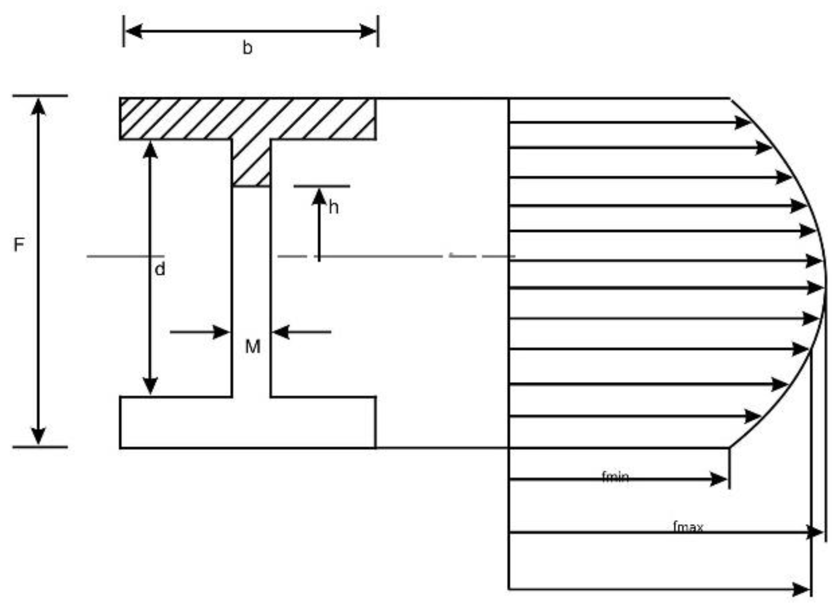
Figure 1.
Based on the classical beam theory, the in-plane displacement of the two parts in the x direction is shown. The maximum deviation in beams is fmax where fmax= (A = bh is the cross-sectional area, V=dM/dx).
Figure 1.
Based on the classical beam theory, the in-plane displacement of the two parts in the x direction is shown. The maximum deviation in beams is fmax where fmax= (A = bh is the cross-sectional area, V=dM/dx).

© 2019 by the author. Licensee MDPI, Basel, Switzerland. This article is an open access article distributed under the terms and conditions of the Creative Commons Attribution (CC BY) license (http://creativecommons.org/licenses/by/4.0/).
Share and Cite
MDPI and ACS Style
Tuz, M. The Existence of Symmetric Positive Solutions of Fourth-Order Elastic Beam Equations. Symmetry 2019, 11, 121. https://doi.org/10.3390/sym11010121
AMA Style
Tuz M. The Existence of Symmetric Positive Solutions of Fourth-Order Elastic Beam Equations. Symmetry. 2019; 11(1):121. https://doi.org/10.3390/sym11010121
Chicago/Turabian StyleTuz, Münevver. 2019. "The Existence of Symmetric Positive Solutions of Fourth-Order Elastic Beam Equations" Symmetry 11, no. 1: 121. https://doi.org/10.3390/sym11010121
Note that from the first issue of 2016, this journal uses article numbers instead of page numbers. See further details here.