Effects of Land Urbanization on Smog Pollution in China: Estimation of Spatial Autoregressive Panel Data Models

Abstract

Studying the impact of land urbanization on smog pollution has important guiding significance for the sustainable development of cities. This study adds the spatial effect between regions into the research framework of smog pollution control in China. On the basis of a panel dataset of 31 province-level administrative regions in China from 2000 to 2017, we investigate the impact of land urbanization on smog pollution. We construct a spatial weight matrix and use Moran’s I statistic and the spatial autoregressive panel data model. The research results show that land urbanization and smog pollution have an inverted U-shaped relationship. With the advancement of land urbanization, the area’s smog pollution first increases and then decreases. However, in general, China has not passed the inflection point and is still at a stage where increasing land urbanization rate aggravates smog pollution. Moreover, the country’s smog pollution has a significant spatial positive correlation that shows agglomeration. In that context, multiple environmental governance entities, including the government, enterprises, and the public, need to collaborate on measures to reduce smog pollution. Future urban construction in China will need to integrate solutions that address the current nexus between urbanization and smog pollution to achieve green and sustainable development.

1. Introduction

Since their reform and opening up, cities in China have been expanding with the continuous growth of the total economic volume [1,2]. The National Bureau of Statistics reported that China’s urbanization rate increased from 17.9% in 1978 to 60.6% in 2019 [3]. However, the rapid growth of the Chinese economy and the expansion of the city scale come at the cost of considerable energy consumption and severe environmental pollution [4,5,6,7], especially smog pollution. Smog is a mixture of smoke and fog, and an important measure of smog pollution is the peak hourly concentrations of ambient fine particulate matter (PM_2.5) [8]. Industrial sectors, such as automobile manufacturing, coal mining, construction and cement manufacturing, are known to generate large quantities of air pollutants, especially PM_2.5 particles [9]. In recent years, smog pollution has occurred frequently, posing a great health hazard to the public [10,11]. Reports show that ambient particulate matter pollution is the fourth-leading risk factor for deaths in China, behind dietary risks, high blood pressure, and smoking [12]. The ever-increasing smog pollution has attracted the attention of the public. Consequently, policymakers have begun to adopt many strategies to control smog pollution. In 2013, the Chinese government deployed 10 measures to prevent and control smog pollution and released the Action Plan for Preventing and Controlling Air Pollution [13,14]. The implementation of these policies has begun to suppress the intensification of smog pollution, but the overall levels of smog are still a cause for concern. The latest data showed that in 2019, the days with PM_2.5 as the main pollutant accounted for 78.8% of the days with severe pollution and above in China, and the days with PM₁₀ as the main pollutant also reached 19.8% [15].

Numerous research results from ecological economics show that the increase in smog pollution is related to many factors, such as economic development, coal consumption, industrial structure, transportation, and environmental governance efficiency [16,17,18,19,20]. The impact of accelerating urbanization on smog pollution needs more special attention than these direct causes of pollution [21]. Urbanization has produced agglomeration effects and promoted economic development, but the rapidly expanding city scale has also brought about “urban diseases,” such as traffic congestion and smog pollution [22]. Previous research results described the relationship between urbanization and atmospheric environment from different perspectives and by using different methods [23,24,25,26]. However, these studies focus on the changes in population size and the impact of social and economic development on the atmospheric environment in the urbanization perspective [27]. Urbanization is a process of transformation of land usable functions [28]. In this process, land plays an extremely important role. Industrial structure adjustment, population agglomeration, and infrastructure construction must be realized through the reconfiguration of land [29,30]. Land urbanization is embodied in the process of converting agricultural land into non-agricultural land and rural land into urban land [31]. Moreover, tracts of natural vegetation (nature-spaces) are also converted at the peri-urban fringe and within the built environment of new and growing cities. The changes in land use patterns and structure, the allocation of land indicators, the resulting changes in economic development space, and the adjustment of industrial structure have an impact on air quality [32].

In addition, spatial factors play an important role that cannot be ignored in the study of environmental economic issues [33]. Due to the existence of natural and geographical factors, such as water flow and wind direction, the environmental problems of an area will inevitably be affected by its neighboring areas. Human factors, such as industrial transfer and trade, further deepen the spatial linkage between regional environmental quality and economic development. Previous studies on the relationship between urbanization and smog pollution confirm the existence of spatial spillover effects of air pollution and its governance [34,35,36]. However, those studies assumed environmental independence between regions, which is inconsistent with reality.

This study advances understanding of the relationship between urbanization and smog pollution in China by adding the spatial effect between regions into the research framework. We propose the first research hypothesis, that is, smog pollution has a significant spatial correlation. According to the Environmental Kuznets Curve (EKC) hypothesis, we propose the second research hypothesis, that is, land urbanization and smog pollution have an inverted U-shaped relationship. On the basis of a panel dataset of 31 province-level administrative regions in China from 2000 to 2017, we constructed a spatial weight matrix and used Moran’s I statistic and spatial autoregressive (SAR) panel data model. We tested these research hypotheses and found the inflection point of the inverted U-shaped curve. With this study, we aim to provide a reference for China’s urban construction and sustainable development.

The remainder of this study is organized as follows. Section 2 introduces the materials and methods commonly used in spatial measurement research, including the spatial weight matrix, Moran’s I statistic, and the SAR panel data model. It also lists the variables and original data sources used in the proposed model. Section 3 presents the results of the research that used software, such as Stata, ArcGIS, and GeoDa, to analyze in detail the spatiotemporal distribution characteristics of smog pollution and land urbanization in China, the spatial autocorrelation of smog pollution, and the impact of land urbanization on smog pollution. It also explains the series of robustness tests conducted on the results. Section 4 discusses the empirical results on the basis of the reality of land urbanization and smog pollution in China. Finally, Section 5 provides a summary of the results and conclusions.

2. Materials and Methods

2.1. Spatial Weights Matrix

The spatial weights matrix is a necessary element in most regression models where a presentation of spatial structure is needed [37]. Common spatial weight matrices include three types: contiguity-based spatial weights, distance-based spatial weights, and economic-based spatial weights [38]. These three spatial weight matrices are defined as follows:

$$w_{ij}^C=\{\begin{array}{l}1, i and j are neighbors\\ 0,i and j are not neighbors\end{array}$$

(1)

$$w_{ij}^D=\{\begin{array}{l}1/d^2,i\ne j\\ 0,i=j\end{array}$$

(2)

$$w_{ij}^E=\{\begin{array}{l}1/\left|pgd{p}_i-pgd{p}_j\right|,i\ne j\\ 0,i=j\end{array}$$

(3)

where i and j are regions, and d is the distance between the geographic centers of the two regions. We selected the location of the provincial capitals. pgdp is per capita GDP. We used contiguity-based spatial weights to reflect whether area i and area j are adjacent, distance-based spatial weights to reflect the geographic spatial distance between area i and area j, and economic-based spatial weights to reflect the economic distance between area i and area j. Following previous research, we mainly chose contiguity-based spatial weights for spatial measurement analysis [39,40]. We also used distance and economic-based spatial weights to test the robustness of the results.

2.2. Moran’s I Statistic

This study uses Moran’s I statistic to examine the spatial autocorrelation of smog pollution. Moran’s I statistic is the most popular test for spatial correlation, including global Moran’s I and local Moran’s I [41,42]. The calculation is formulated as follows:

$$I=\frac{n{\sum }_{i=1}^n{\sum }_{j=1}^n{w}_{ij}\left({\rho }_i-\overline{\rho }\right)\left({\rho }_j-\overline{\rho }\right)}{{\sum }_{i=1}^n{\sum }_{j=1}^n{w}_{ij}{\sum }_{i=1}^n{\left({\rho }_i-\overline{\rho }\right)}^2}$$

(4)

$$I_i=\frac{{\rho }_i-\overline{\rho }}{S^2}·{\sum }_{j\ne i}{w}_{ij}\left({\rho }_j-\overline{\rho }\right),\mathrm{which}{S}^2=\frac{{\sum }_i{\left({\rho }_i-\overline{\rho }\right)}^2}{n}$$

(5)

where ${\rho }_i$ is smog pollution of area I, $\overline{\rho }$ is the mean of smog pollution, $w_{ij}$ is the spatial weights matrix. The value range of Moran’s I statistic is from −1 to 1, and a value greater than 0 indicates spatial positive correlation, that is, the spatial distribution characteristics of high value and high value aggregation or low value and low value aggregation. By contrast, a value less than 0 is a spatial negative correlation, that is, a spatial distribution characteristic in which a high value surrounds a low value or a low value around a high value. A value equal to 0 is irrelevant. To investigate the local spatial autocorrelation of smog pollution, we further used Stata to generate a local Moran scatter plot maps of China’s smog pollution for each year. We also used GeoDa and ArcGIS to produce local indicators of spatial association (LISA) agglomeration maps of smog pollution for each year.

2.3. SAR Panel Data Model

The SAR panel data model is used to estimate the impact of land urbanization on smog pollution. The traditional panel measurement model does not consider the possible spatial correlation of dependent variables. From the perspective of externality, the SAR panel data model examines the impact of changes in a region’s elements from other regions. The SAR panel data model in this study is defined as follows:

$$smo{g}_{it}=u_i+{\gamma }_t+\rho w_i^{\prime }smo{g}_t+{\beta }_{1}landurba{n}_{it}+{\beta }_{2}landurba{n}_{it}^2+{\beta }^{\prime }contro{l}_{it}^{\prime }+{\epsilon }_{it}$$

(6)

where i is the region; t is the time; smog is the dependent variable, that is, smog pollution; landurban is the independent variable that this study focuses on, that is, land urbanization; control refers to all control variables; $u_i$ and ${\gamma }_t$ represent individual effects and time effects, respectively. According to the EKC hypothesis, we add the quadratic term of land urbanization to the proposed model to investigate the possible non-linear effects of land urbanization on smog pollution. ${\beta }_1$, ${\beta }_2$ and ${\beta }^{\prime }$ are the coefficients of each variable [43,44].

2.4. Variable Definitions and Data Description

The eight variables included in the SAR panel data model constructed through this study (

Table 1. Variable definitions.

Types	Variables	Symbol
Dependent variable	PM2.5 concentration (μg/m3)	PM2.5
Independent variable	Land urbanization rate (%)	landurban
	Square of land urbanization rate	landurban2
Control variable	Population per km2 (logarithm)	lnpop
	Per capita gross domestic product (logarithm)	lnpgdp
	Number of patent application authorization (logarithm)	lnrd
	Proportion of the added value of tertiary industry to GDP (%)	third
	Number of college students per 10,000 people (logarithm)	lnedu
	Proportion of total imports and exports to GDP (%)	open

Note: Symbols are set in italics to distinguish them from the main text.

) are:

(1)

Dependent variable: Smog pollution is the dependent variable in the proposed model. We selected the PM_2.5 concentration, which is the main source of smog pollution and that which most concerns the Chinese public, as the measurement index. The original data come from the American Atmospheric Composition Analysis Group. The data type is gridded datasets (resolution is 0.01° × 0.01°) [45]. We used ArcGIS to analyze the original data packet and match them with the maps of China’s provinces to obtain the average PM_2.5 concentration. Finally, we obtained the panel datasets of 31 province-level administrative regions in China from 2000 to 2017. The advantage of this analysis is the comprehensive integration of satellite monitoring data and ground monitoring data, which can accurately and objectively reflect the true situation of China’s smog pollution.

(2)

Independent variable: Land urbanization is the independent variable that this article focuses on. With reference to Liu and Wang’s approach [46,47], we used land urbanization rate in the measurement, and the specific calculation formula is as follows:

$$landurba{n}_{it}=\frac{Uare{a}_{it}}{Tare{a}_{it}}\times 100\%$$

(7)

where i is the region, t is the time, Uarea is the built-up area of each province’s city, and Tarea is the total land area of each province.

(3)

Control variable: To improve the accuracy of the model estimation results, we selected some relevant factors that may affect smog pollution as control variables and put them in the model. First, considering the traditional stochastic impacts by regression on population, affluence, and technology (STIRPAT) model, we controlled the impact of population, wealth, and technology on smog pollution [48,49]. Second, we measured the demographic factor by the population per km², the wealth factor by per capita GDP, and the technical factor by the number of patent application authorizations. Third, informed by other studies, we considered the impact of industrial structure, education level, and degree of openness on smog pollution [50,51,52]. We model industrial structure by the proportion of the added value of tertiary industry to GDP, the education level by the number of college students per 10,000 people, and the degree of openness by the proportion of total import and export to GDP.

After data collection, this study analyzed the panel dataset of 31 provincial administrative regions in China from 2000 to 2017. Due to the lack of data, the research area of this study does not include Hong Kong, Macau, and Taiwan.

Table 2. Descriptive statistics and multicollinearity test.

Variable	Obs	Mean	SD	Min	Max	VIF
PM2.5	558	38.06	16.30	4.730	84.50	—
landurban	558	1.547	2.770	0.00562	15.75	4.16
lnpop	558	5.266	1.477	0.742	8.249	4.23
lnpgdp	558	10.01	0.841	7.887	11.77	7.79
lnrd	558	8.589	1.837	1.946	12.72	5.07
third	558	41.66	8.546	28.60	80.56	2.05
lnedu	558	4.835	0.589	3.055	5.876	4.10
open	558	30.47	38.15	1.688	172.2	2.55

lists the descriptive statistical and multicollinearity test of all the original data. According to the results of variance inflation factor (VIF), the VIF of the independent variable and all the control variables are less than 10, thereby indicating that the variables selected in this paper do not have multicollinearity [26,53].

3. Results

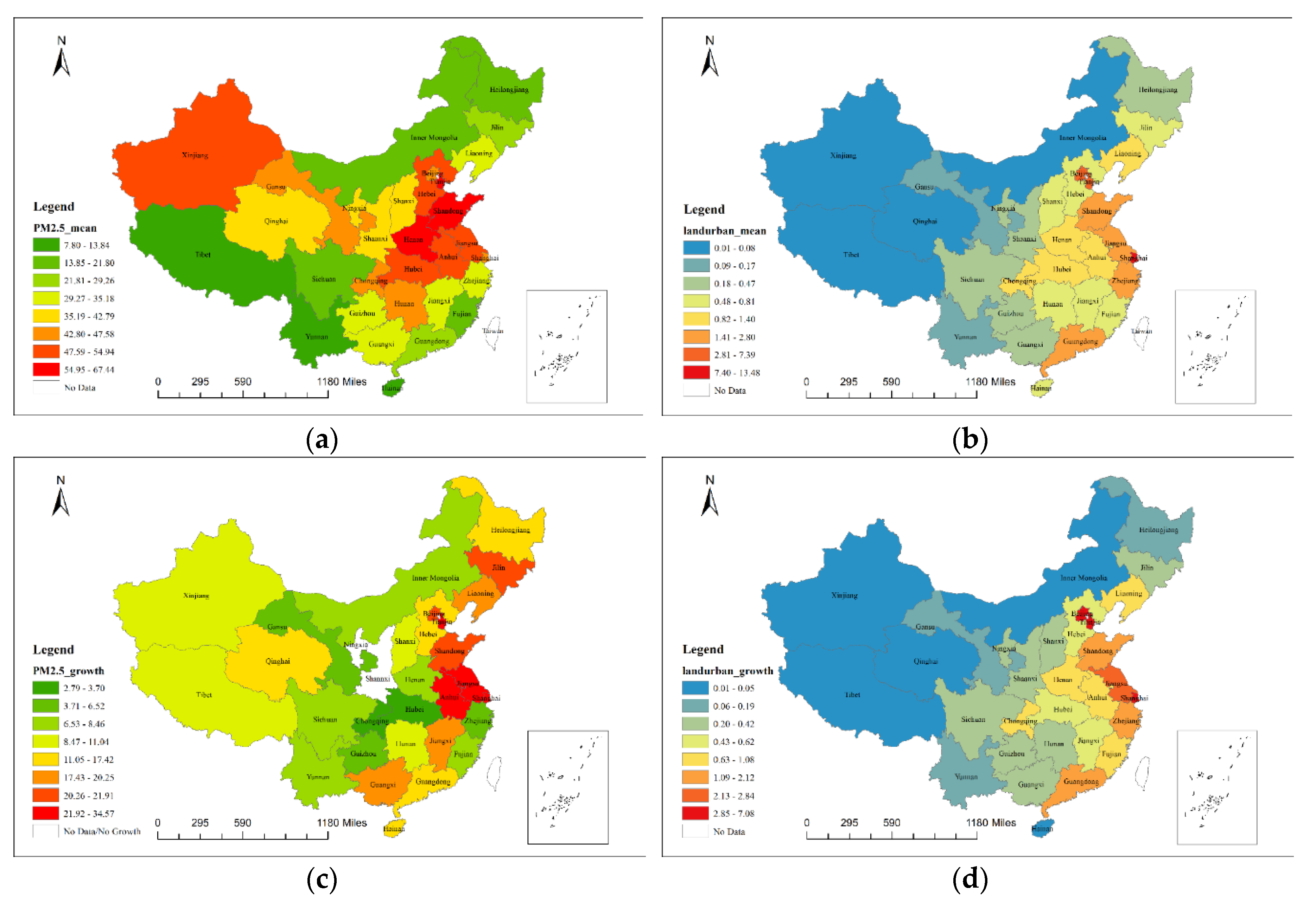
3.1. Spatiotemporal Distribution of Land Urbanization and Smog Pollution

Figure 1 displays the spatial distribution characteristics of land urbanization and smog pollution in China wherein (a) and (b) reflect the mean distribution, and (c) and (d) reflect the distribution of growth. The areas with severe smog pollution are mainly concentrated in the four regions: Central, North, East, and Northwest China. Northeast, Southwest, and South China have small degrees of smog pollution. From the perspective of changes, smog pollution is rapidly increasing in various areas, including Beijing, Tianjin, Shanghai, Shandong, Jiangsu, Anhui, and Jilin. The growth of PM_2.5 in all area exceeds 20 μg/m³, and in some areas even exceeds 50 μg/m³. In terms of land urbanization, the mean and the growth distributions show an increasing distribution characteristic from west to east. This finding is also consistent with the distribution of regional differences in China’s economic development level.

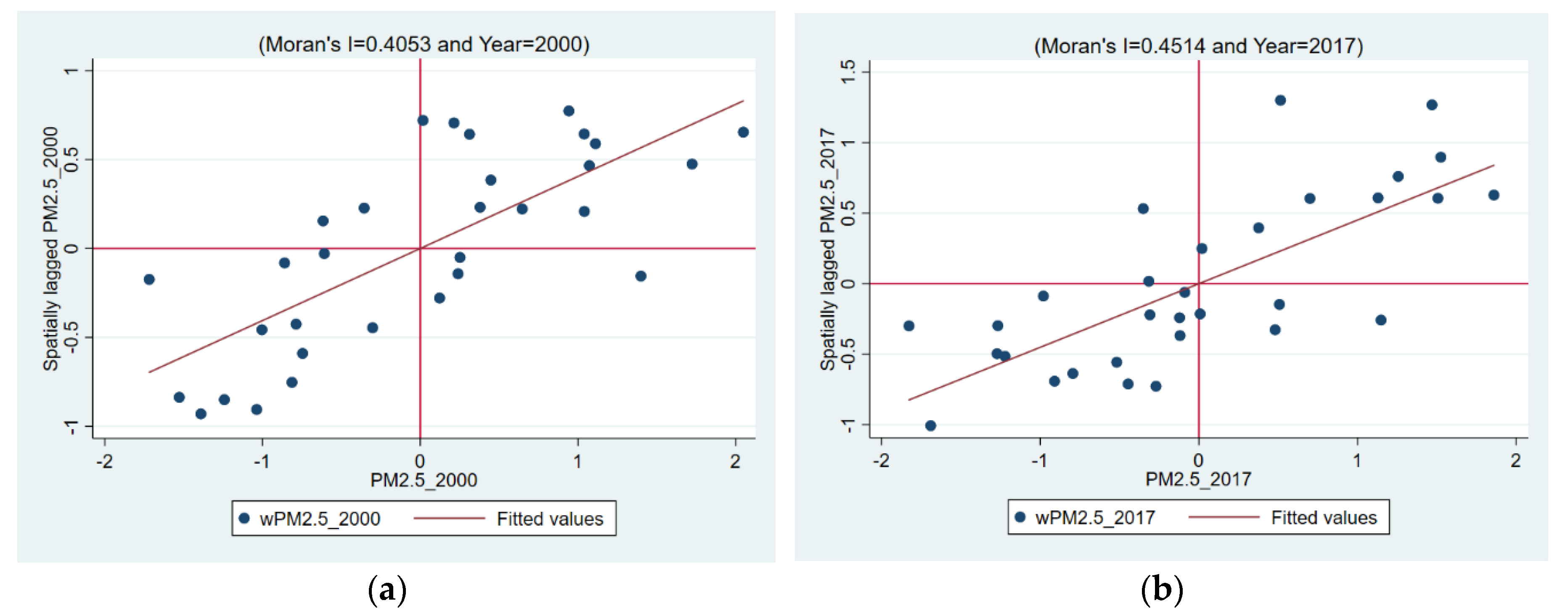
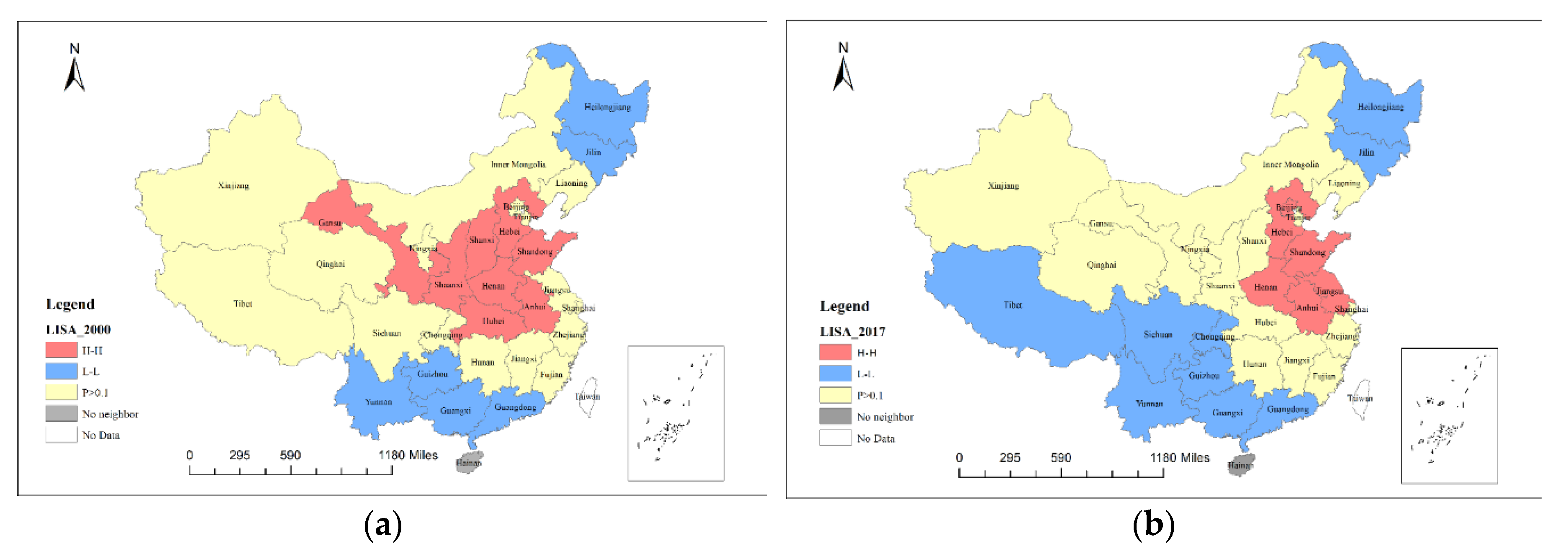
3.2. Spatial Autocorrelation of Smog Pollution

We used Stata to measure the global Moran’s I of China’s PM_2.5 concentration from 2000 to 2017. The test results reported in

Table 3. Global Moran’s I of China’s PM_2.5 concentration, 2000–2017.

Year	Global Moran’s I	Z-Statistic	p-Value	Sig
2000	0.405	3.653	0.000	***
2001	0.434	3.877	0.000	***
2002	0.432	3.867	0.000	***
2003	0.486	4.333	0.000	***
2004	0.409	3.693	0.000	***
2005	0.451	4.046	0.000	***
2006	0.498	4.455	0.000	***
2007	0.500	4.464	0.000	***
2008	0.453	4.067	0.000	***
2009	0.448	4.045	0.000	***
2010	0.425	3.838	0.000	***
2011	0.496	4.423	0.000	***
2012	0.444	3.990	0.000	***
2013	0.493	4.419	0.000	***
2014	0.417	3.762	0.000	***
2015	0.486	4.341	0.000	***
2016	0.505	4.511	0.000	***
2017	0.451	4.041	0.000	***

Note: *** p < 0.01.

show that the global Moran index values over the years are roughly distributed between 0.4–0.5 and all passed the 1% significance test. Thus, China’s smog pollution shows a significant positive spatial correlation. The spatial distribution of smog pollution in China presents the “club” distribution characteristics of high value and high value agglomeration and low value and low value agglomeration. This result also indicates the necessity of adding spatial influencing factors to the measurement model that examines the impact of land urbanization on smog pollution.

Figure 2 and Figure 3 show local Moran scatter plot maps and LISA agglomeration maps of China’s smog pollution. Due to space limitations, this article only shows the results at the beginning (2000) and the end (2017) of the investigation period.

The results of the Moran scatter plot map show that whether in 2000 or 2017, the local Moran’s I of most provinces are distributed in the first quadrant characterized by high–high agglomeration and the third quadrant characterized by low–low agglomeration. The results of the LISA agglomeration map show that, in terms of spatial distribution, the high-value accumulation areas of smog pollution are mainly distributed in the northern and central provinces of China. By contrast, the low-value accumulation areas of smog pollution are distributed in the northeast and the southwest and southern provinces. In terms of dynamic changes, the high-value agglomeration areas of smog pollution are shrinking, and the pollution center is shifting from the central and western regions to the east. Specifically, Gansu, Shaanxi, Shanxi, and Hubei in the central and western regions withdrew from high-value groups, whereas Beijing and Jiangsu in the eastern regions joined. Although the low-value accumulation areas of smog pollution in the northeast have not changed (Heilongjiang and Jilin), the low-value accumulation areas of smog pollution in the south and southwest have expanded. Compared with the data gathered in 2000, Chongqing, Sichuan, and Tibet also joined the low-value group of smog pollution in 2017.

3.3. Regression Results

Table 4. Estimation results of the spatial autoregressive (SAR) panel data model.

	(1)	(2)	(3)	(4)
W * PM2.5	0.7459 ***	0.7392 ***	0.7282 ***	0.7407 ***
	(0.0325)	(0.0332)	(0.0340)	(0.0332)
landurban	0.6292 ***	1.4049 ***	2.1935 ***	2.2452 ***
	(0.2086)	(0.5274)	(0.5938)	(0.6060)
landurban2		−0.0391 *	−0.0611 **	−0.0677 **
		(0.0244)	(0.0259)	(0.0266)
lnpop			−13.1397 ***	−19.4974 ***
			(3.4545)	(3.6331)
lnpgdp			−3.6263 ***	−4.6639 ***
			(1.2787)	(1.3778)
lnrd			0.0166	0.0978
			(0.4676)	(0.4654)
third				−0.2035 ***
				(0.0470)
lnedu				−3.8029 ***
				(1.1180)
open				−0.0194
				(0.0129)
Ind fixed	Yes	Yes	Yes	Yes
Time fixed	Yes	Yes	Yes	Yes
N	558	558	558	558
R2	0.2176	0.2301	0.1462	0.1937
Inflection point		17.96	17.95	16.58
Cross the inflection point		None	None	None

Note: Standard errors in parentheses. *** p < 0.01, ** p < 0.05, * p < 0.1.

reports the estimation results of the SAR panel data model under different conditions. Columns 1 and 2 are the estimation results without the addition of control variables. The difference between Columns 1 and 2 adds a quadratic term with the dependent variable to the model to examine whether land urbanization has a nonlinear impact on smog pollution. Column 3 is the estimated result after adding control variables on the basis of the STIRPAT model, and Column 4 is the estimated result after adding all control variables to the model. From the results in Table 4, we can conclude the following:

(1)

The estimation results in Columns 1–4 show that under different constraint conditions, the estimated coefficient of W * PM_2.5 is significantly positive, thereby indicating that China’s smog pollution has a significant positive spatial correlation. This result is consistent with Moran’s I test result. The estimated coefficient value shows that an increase of 1 μg/m³ in the PM_2.5 concentration in the neighborhood increases the local PM_2.5 concentration by more than 0.7 μg/m³.

(2)

The estimation results in Columns 2–4 show that without the addition of control variables, the estimated coefficient of the first-order term of landurban is significantly positive. By contrast, the estimated coefficient of the quadratic term is significantly negative. After gradually adding the control variables, the estimated coefficient of the first-order term of landurban is still significantly positive. The estimated coefficient of the quadratic term is still significantly negative. These results indicate that land urbanization has a nonlinear impact on smog pollution. Specifically, land urbanization and smog pollution have an inverted U-shaped relationship, that is, with the increase in land urbanization rate, the level of smog pollution shows a trend of first rising and then falling.

(3)

The estimated results in Columns 3–4 also show the impact of each control variable on smog pollution. The estimated coefficients of lnpop, lnpgdp, third, and lnedu are all significantly negative, thereby indicating that the improvement of regional economic level, the agglomeration effect brought about by the increase in population size, the improvements of industrial structure and education level significantly reduce the concentration of PM_2.5 in the region. The estimated coefficients of lnrd and open fail to pass the significance test. As far as the data used in this study are concerned, the evidence to prove that the level of technology and openness of the region have a statistically significant impact on smog pollution is insufficient.

The estimation results of the SAR panel data model show that land urbanization and smog pollution have an inverted U-shaped relationship. We aimed to find the inflection point of this inverted U-shaped relationship and identify the provinces that have crossed this inflection point. On the basis of the regression results in Table 4, we calculated the inflection point values of the inverted U-shaped curve in Columns 2–4, which are 17.96, 17.95, and 16.58, respectively. Compared with the original data, we find that as of the end of the investigation period (2017), no area has crossed the inflection point and entered the stage where increasing land urbanization promotes the improvement of smog pollution. Moreover, most areas are still far from the inflection point. This result indicates that although land urbanization and smog pollution have an inverted U-shaped relationship, China is still on the left of this inverted U-shaped curve as a whole, that is, increasing land urbanization rate aggravates smog pollution.

3.4. Robustness Test

3.4.1. Change the Regression Method

To verify the robustness of the conclusions drawn in Section 3.3, we performed a series of tests. We changed the regression method to re-estimate the coefficients of the independent variables in the proposed model.

Table 5. Estimated results of different methods.

	OLS	PSEM	PSAC	PSDM
landurban	5.4874 ***	8.3873 ***	9.0453 ***	1.7832 ***
	(0.8481)	(1.0444)	(1.0890)	(0.6627)
landurban2	−0.1955 ***	−0.3972 ***	−0.4159 ***	−0.0497 *
	(0.0374)	(0.0510)	(0.0519)	(0.0289)
Control variable	Yes	Yes	Yes	Yes
Ind fixed	Yes	Yes	Yes	Yes
Time fixed	Yes	Yes	Yes	Yes
N	558	558	558	558
R2	0.5772	0.2605	0.1466	0.1640
Inflection point	14.03	10.56	10.01	17.94
Cross the inflection point	Shanghai	Shanghai	Shanghai	None

Note: Standard errors in parentheses. *** p < 0.01, * p < 0.1. Due to space limitations, the estimated results of the control variables are not listed in the table. The complete estimated results can be found in Appendix A.

lists the estimated results. Column 1 is the Ordinary Least Squares (OLS)method not considering the spatial correlation, and Columns 2–4 are the other three panel space measurement models. They are the Panel Space Error Model (PSEM) that only contains the spatial autocorrelation of the error term, the Panel Space Autocorrelation Model (PSAC) that contains the spatial lag of the explained variable and the spatial autocorrelation of the error term, and the Panel Space Dubin Model (PSDM) that considers the spatial lag of independent variables on the basis of SAR panel data model. Table 5 shows that no matter which method is used, the estimated coefficient of the first-order term of the independent variable landurban, which is the focus of this study, is significantly positive. By contrast, the estimated coefficient of the quadratic term is significantly negative. On the basis of the estimation results of OLS, PSEM, and PSAC, only Shanghai has passed the inflection point. The PSDM estimation results are consistent with SAR panel data model, and no province passed the inflection point.

3.4.2. Change the Spatial Weight Matrix

For the spatial measurement model, the choice of the spatial weight matrix has a great impact on the results. To test this influence, we re-estimated the SAR panel data model by changing the spatial weight matrix. Columns 1–2 of

Table 6. SAR panel data model estimated results of different spatial weight matrices.

	Distance	Economic
landurban	3.4904 ***	5.9174 ***
	(0.6671)	(0.8228)
landurban2	−0.1226 ***	−0.2131 ***
	(0.0292)	(0.0362)
Control variable	Yes	Yes
Ind fixed	Yes	Yes
Time fixed	Yes	Yes
N	558	558
R2	0.1771	0.1821
Inflection point	14.23	13.88
Cross the inflection point	Shanghai	Shanghai

Note: Standard errors in parentheses. *** p < 0.01. Due to space limitations, the estimated results of the control variables are not listed in the table. The complete estimated results can be found in Appendix A.

are the estimated results by using the distance and economic-based spatial weights. Table 6 shows that no matter which spatial weight matrix is used, the estimated coefficient of the first-order term of landurban is significantly positive, and the estimated coefficient of the quadratic term is significantly negative. Land urbanization and smog pollution have maintained a significant inverted U-shaped relationship. The calculation result of the inflection point shows that only Shanghai has passed the inflection point and entered the right half of the inverted U-shaped curve. In general, the abovementioned series of tests proved that the conclusions drawn in this article are robust.

4. Discussion

4.1. The Inverted U-Shaped Relationship between Land Urbanization and Smog Pollution

The estimation results of the SAR panel data model show that land urbanization and smog pollution have an inverted U-shaped relationship. From other perspectives of urbanization, such as population urbanization, the results of this study are similar to the previous research. For example, Liu et al. (2015) found the same inverted U-shaped relationship between population agglomeration brought about by urbanization and smog pollution by using panel threshold model [54]. Based on the structural equation model, Li et al. (2017) also found that the impact of urban population density on smog pollution shows as an inverted U-shape [55]. Moreover, the results of this study are also different from the previous research. In Wang’s (2019) research, he found that there is a significant U-shaped relationship between land urbanization and atmospheric ecological environment quality. The reason for this difference may be that he used SO₂ emissions to define air pollution [56]. This study expands the research on the impact of urbanization on smog pollution and indicates that the relationship between land urbanization and smog pollution conforms to the EKC hypothesis, as an important feature of economic development. Referring to previous studies, we can discuss this influence mechanism. In periods when low land urbanization is rate, the regional economic development level is low, the technical level is not high, the industrial structure level is low, and the economic development is mainly based on the extensive development model [56]. The central government assesses local governments with economic development indicators, such as GDP and taxes. To increase the total amount of local GDP and taxes, the local governments allocate the indicators of construction land to industrial land in the secondary industry [57]. However, industrial land causes great air pollution [58]. In periods of high land urbanization rate, the local economy has developed to an advanced stage, and the development model is mainly characterized by intensive development [59]. The government and urban residents are aware of the importance of environmental protection, and the reality of high pollution forces the central government to issue environmental regulations and policies to restrict the development of industries in various regions. To meet the requirements of the central government’s environmental regulations and policies, local governments’ land and industrial policies favor the service industry and high-tech industries in the tertiary industry. Local governments also reduce the proportion of industrial land transfers and allocate considerable construction land indicators to tertiary industry land, thereby reducing pollutant emissions and realizing economic transformation and green development [56].

4.2. The Current Stage of China

By calculating the inflection point, we find that China is still at a stage where increasing land urbanization rate exacerbates smog pollution, although land urbanization and smog pollution have an inverted U-shaped relationship. The contradiction between urban development and smog pollution is still prominent, and thus resolving this contradiction is an important issue currently in China’s urban construction. According to the theory of ecological modernization, urbanization essentially embodies the modernization of individuals and societies. The mitigation of environmental problems, such as air pollution, is the result of the joint efforts of various actors at multiple levels in the process of balancing economic development and environmental protection [60]. These actors include government, enterprises, and the public. To formulate a reasonable urban plan, the government cannot blindly pursue the expansion of the city scale [61]. Instead, policymakers need to focus on the compact and intensive development of cities [22]. In addition, a series of policies is needed to guide the development of urban industrial structure and promote the rational allocation of urban resources. Enterprises need to enhance their sense of social responsibility and continuously reduce the proportion of industries with high energy consumption, high pollution, and high emissions. In addition, they must strengthen the research and development of pollution control technologies to realize clean and sustainable production methods [62]. As far as the public is concerned, they must take on the responsibility of supervising the government and enterprises and promoting environmental protection awareness and knowledge. The public should not simply regard themselves as the victims of smog pollution, but more importantly, realize how to move from a comfortable but high energy consumption lifestyle to a green and sustainable way of life and consumption as citizens [63,64]. Through the joint efforts of different governance entities, the positive externalities of regional, social, and economic development brought about by land urbanization on smog pollution can be stimulated, and a win–win situation between urban development and smog governance can be realized.

4.3. The Positive Spatial Correlation of Smog Pollution in China

A series of spatial measurement methods indicate that China’s smog pollution has a significant positive spatial correlation that shows agglomeration. One or more higher areas are adjacent to a high area. Similarly, at least one lower area is adjacent to a low area. The results of the global Moran’s I show that from 2000 to 2017, the positive spatial correlation of smog pollution fluctuated between 0.4 and 0.5, indicating that this spatial correlation continues to be at a high level. The SAR panel data modelling of this study shows that increase of 1 μg/m³ in the PM_2.5 concentration in a neighboring region increases the local PM_2.5 concentration by 0.7407 μg/m³. This study demonstrates that in the process of smog pollution control, local governments should not only focus on the remediation of “heavy-hit areas,” such as North and Central China. They should also realize that the control of smog is not the responsibility of a certain province [65]. The spatial relevance of smog pollution requires each province to break down their own administrative barriers; strengthen regional cooperation and information sharing; promote the flow of technology, talent, capital, and other elements of smog governance among different regions; and improve the efficiency of smog governance to comprehensively improve China’s smog pollution problem [66,67].

5. Conclusions

This study adds the spatial effect between regions into the research framework of smog pollution control in China. On the basis of a panel dataset of 31 province-level administrative regions in China from 2000 to 2017, we investigated the impact of land urbanization on smog pollution. We constructed a spatial weight matrix and used Moran’s I statistic and the SAR panel data model. The modelling of this study demonstrates that land urbanization and smog pollution have an inverted U-shaped relationship. With the advancement of land urbanization, an area’s smog pollution first increases and then decreases. However, in general, China has not passed the inflection point and is still at a stage where increasing land urbanization rate aggravates smog pollution. Moreover, the country’s smog pollution has a significant spatial positive correlation that shows agglomeration. That evidence of agglomeration means that an increase in smog pollution in one city or region will lead to an increase in smog pollution in neighboring cities and regions.

While advancing smog pollution research in China, there are some shortcomings in this study. For example, due to the difficulty of collecting data, this article still uses the panel dataset at the provincial level in China. If a city-level panel dataset can be used in future research, it will more objectively reflect the relationship between land urbanization and smog pollution in China. In addition, the existence of this inverted U-shaped relationship between land urbanization and smog pollution does not mean that the smog pollution problem will be automatically solved when the land urbanization rate exceeds a certain level. Instead, multiple environmental governance entities, including the government, enterprises, and the public, need to collaborate on measures to reduce smog pollution. In that context, future urban construction in China will need to integrate solutions that address the current nexus between urbanization and smog pollution to achieve green and sustainable development.

References

1. Gu, C.L.; Pang, H.F. Evolution of Chinese urbanization spaces: Kernel spatial approach. Sci. Geogr. Sin. 2009, 29, 10–14. [Google Scholar] [CrossRef]
2. Liu, Z.F.; He, C.Y.; Zhang, Q.F.; Huang, Q.X.; Yang, Y. Extracting the dynamics of urban expansion in China using DMSP-OLS nighttime light data from 1992 to 2008. Landsc. Urban Plan 2012, 106, 62–72. [Google Scholar] [CrossRef]
3. NBS. China Statistical Yearbook; China Statistics Press: Beijing, China, 2018.
4. Peng, S.J.; Bao, Q. Economic growth and environmental pollution: An empirical test for the environmental Kuznets curve hypothesis in China. Res. Financ. Econ. Issues 2006, 8, 3–17. [Google Scholar] [CrossRef]
5. Rao, C.J.; Yan, B.J. Study on the interactive influence between economic growth and environmental pollution. Environ. Sci Pollut. R. 2020. [Google Scholar] [CrossRef] [PubMed]
6. Wu, Y.; Zhu, Q.W.; Zhu, B.Z. Comparisons of decoupling trends of global economic growth and energy consumption between developed and developing countries. Energy Policy 2018, 116, 30–38. [Google Scholar] [CrossRef]
7. Wang, S.J.; Li, Q.Y.; Fang, C.L.; Zhou, C.S. The relationship between economic growth, energy consumption, and CO2 emissions: Empirical evidence from China. Sci. Total Environ. 2016, 542, 360–371. [Google Scholar] [CrossRef]
8. Zhou, M.G.; He, G.J.; Fan, M.Y.; Wang, Z.X.; Liu, Y.; Ma, J.; Ma, Z.W.; Liu, J.M.; Liu, Y.N.; Wang, L.H.; et al. Smog episodes, fine particulate pollution and mortality in China. Enviton. Res. 2015, 136, 396–404. [Google Scholar] [CrossRef]
9. David, H.; Jiang, J.Y. A study of smog issues and PM2.5 pollutant control strategies in China. J. Environ. Prot. 2013, 4, 746–752. [Google Scholar] [CrossRef] [Green Version]
10. Sram, R.J.; Binkova, B.; Dostal, M.; Merkerova-Dostalova, M.; Libalova, H.; Milcova, A.; Rossner, P.; Rossnerova, A.; Schmuczerova, J.; Svecova, V.; et al. Health impact of air pollution to children. Int. J. Hyg. Environ. Health 2013, 216, 533–540. [Google Scholar] [CrossRef]
11. Matus, K.; Nam, K.M.; Selin, N.E.; Lamsal, L.N.; Reilly, J.M.; Paltsev, S. Health damages from air pollution in China. Glob. Environ. Chang. 2012, 22, 55–66. [Google Scholar] [CrossRef] [Green Version]
12. Wong, E. Air Pollution Linked to 1.2 Million Premature Deaths in China. Available online: https://www.nytimes.com/2013/04/02/world/asia/air-pollution-linked-to-1-2-million-deaths-in-china.html (accessed on 12 July 2020).
13. Zhang, D.Y.; Liu, J.J.; Li, B.J. Tackling air pollution in China—What do we learn from the great smog of 1950s in London. Sustainability 2014, 6, 5322–5338. [Google Scholar] [CrossRef] [Green Version]
14. Huang, R.J.; Zhang, Y.L.; Bozzetti, C.; Ho, K.F.; Cao, J.J.; Han, Y.M.; Daellenbach, K.R.; Slowik, J.G.; Platt, S.M.; Canonaco, F. High secondary aerosol contribution to particulate pollution during haze events in China. Nature 2014, 514, 218–222. [Google Scholar] [CrossRef] [Green Version]
15. CMEE. Bulletin on the State of China’s Ecological Environment in 2019. Available online: http://www.mee.gov.cn/hjzl/sthjzk/zghjzkgb/202006/P020200602509464172096.pdf (accessed on 11 August 2020).
16. Sueyoshi, T.; Yuan, Y. China‘s regional sustainability and diversified resource allocation: DEA environmental assessment on economic development and air pollution. Energy. Econ. 2015, 49, 239–256. [Google Scholar] [CrossRef]
17. Qi, Y.; Stern, N.; Wu, T.; Lu, J.Q.; Green, F. China‘s post-coal growth. Nat. Geosci. 2016, 9, 564–566. [Google Scholar] [CrossRef] [Green Version]
18. Wang, K.L.; Miao, Z.; Zhao, M.S.; Miao, C.L.; Wang, Q.W. China’s provincial total-factor air pollution emission efficiency evaluation, dynamic evolution and influencing factors. Ecol. Indic. 2019, 107, 105578. [Google Scholar] [CrossRef]
19. Gurram, S.; Stuart, A.L.; Pinjari, A.R. Agent-based modeling to estimate exposures to urban air pollution from transportation: Exposure disparities and impacts of high-resolution data. Comput. Environ. Urban 2019, 75, 22–34. [Google Scholar] [CrossRef]
20. Betsill, M.M.; Bulkeley, H. Transnational networks and global environmental governance: The cities for climate protection program. Int. Stud. Q. 2004, 48, 471–493. [Google Scholar] [CrossRef]
21. Parrish, D.D.; Stockwell, W.R. Urbanization and air pollution: Then and now. Earth Space Science News 2015, 96. [Google Scholar] [CrossRef]
22. Shao, S.; Li, X.; Cao, J.H. Urbanization promotion and haze pollution governance in China. Econ. Res. J. 2019, 54, 148–165. [Google Scholar]
23. Liu, Y.; Arp, H.P.H.; Song, X.D.; Song, Y. Research on the relationship between urban form and urban smog in China. Environ. Plan B Urban 2017, 44, 328–342. [Google Scholar] [CrossRef]
24. Wang, S.J.; Gao, S.; Li, S.J.; Feng, K.S. Strategizing the relation between urbanization and air pollution: Empirical evidence from global countries. J. Clean. Prod. 2020, 243, 118615. [Google Scholar] [CrossRef]
25. Barbera, E.; Curro, C.; Valenti, G. A hyperbolic model for the effects of urbanization on air pollution. Appl. Math. Model. 2010, 34, 2192–2202. [Google Scholar] [CrossRef] [Green Version]
26. Fang, C.L.; Liu, H.M.; Li, G.D.; Sun, D.Q.; Miao, Z. Estimating the Impact of Urbanization on Air Quality in China Using Spatial Regression Models. Sustainability 2015, 7, 15570–15592. [Google Scholar] [CrossRef] [Green Version]
27. Liang, W.; Yang, M. Urbanization, economic growth and environmental pollution: Evidence from China. Sustain. Comput. Inform. 2019, 21, 1–9. [Google Scholar] [CrossRef]
28. Lv, P.; Zhou, T.; Zhang, Z.F.; Tian, Z. Construction and application of land urbanization and corresponding measurement index system. China Land Sci. 2008, 22, 24–28+42. [Google Scholar] [CrossRef]
29. Lin, X.Q.; Wang, Y.; Wang, S.J.; Wang, D. Spatial differences and driving forces of land urbanization in China. J. Geogr. Sci. 2015, 25, 545–558. [Google Scholar] [CrossRef]
30. Mohan, M.; Pathan, S.K.; Narendrareddy, K.; Kandya, A.; Pandey, S. Dynamics of urbanization and its impact on land-use/land-cover: A case study of megacity Delhi. J. Environ. Prot. 2011, 2, 1274. [Google Scholar] [CrossRef] [Green Version]
31. Deng, X.Z.; Huang, J.K.; Rozelle, S.; Zhang, J.P.; Li, Z.H. Impact of urbanization on cultivated land changes in China. Land Use Policy 2015, 45, 1–7. [Google Scholar] [CrossRef]
32. Wei, Y.D.; Ye, X.Y. Urbanization, urban land expansion and environmental change in China. Stoch Environ. Res. Risk A 2014, 28, 757–765. [Google Scholar] [CrossRef]
33. Anselin, L. Spatial effects in econometric practice in environmental and resource economics. Am. J. Agric. Econ. 2001, 83, 705–710. [Google Scholar] [CrossRef]
34. Fang, D.L.; Chen, B.; Hubacek, K.; Ni, R.J.; Chen, L.L.; Feng, K.S.; Lin, J.T. Clean air for some: Unintended spillover effects of regional air pollution policies. Sci. Adv. 2019, 5, 4707. [Google Scholar] [CrossRef] [Green Version]
35. Feng, T.; Du, H.B.; Lin, Z.G.; Zuo, J. Spatial spillover effects of environmental regulations on air pollution: Evidence from urban agglomerations in China. J. Environ. Manag. 2020, 272, 110998. [Google Scholar] [CrossRef] [PubMed]
36. Jerrett, M.; Burnett, R.T.; Beckerman, B.S.; Turner, M.C.; Krewski, D.; Thurston, G.; Martin, R.V.; van Donkelaar, A.; Hughes, E.; Shi, Y.L.; et al. Spatial Analysis of Air Pollution and Mortality in California. Am. J. Respir. Crit. Care Med. 2013, 188, 593–599. [Google Scholar] [CrossRef] [PubMed]
37. Getis, A.; Aldstadt, J. Constructing the spatial weights matrix using a local statistic. Geogr. Anal. 2004, 36, 90–104. [Google Scholar] [CrossRef]
38. Getis, A. Spatial weights matrices. Geogr. Anal. 2009, 41, 404–410. [Google Scholar] [CrossRef]
39. Anselin, L.; Rey, S.J.; Li, W.W. Metadata and provenance for spatial analysis: The case of spatial weights. Int. J. Geogr. Inf. Sci. 2014, 28, 2261–2280. [Google Scholar] [CrossRef]
40. Anselin, L.; Kim, Y.W.; Syabri, I. Web-based analytical tools for the exploration of spatial data. J. Geogr. Syst. 2004, 6, 197–218. [Google Scholar] [CrossRef]
41. Bivand, R.; Müller, W.G.; Reder, M. Power calculations for global and local Moran’s I. Comput. Stat. Data Anal. 2009, 53, 2859–2872. [Google Scholar] [CrossRef]
42. Anselin, L. Local indicators of spatial association—LISA. Geogr. Anal. 1995, 27, 93–115. [Google Scholar] [CrossRef]
43. Belotti, F.; Hughes, G.; Mortari, A.P. Spatial panel-data models using Stata. Stat. J. 2017, 17, 139–180. [Google Scholar] [CrossRef] [Green Version]
44. Lee, L.F.; Yu, J.H. Estimation of spatial autoregressive panel data models with fixed effects. J. Econom. 2010, 154, 165–185. [Google Scholar] [CrossRef]
45. Hammer, M.S.; van Donkelaar, A.; Li, C.; Lyapustin, A.; Sayer, A.M.; Hsu, N.C.; Levy, R.C.; Garay, M.J.; Kalashnikova, O.V.; Kahn, R.A.; et al. Global Estimates and Long-Term Trends of Fine Particulate Matter Concentrations (1998-2018). Environ. Sci. Technol. 2020, 54, 7879–7890. [Google Scholar] [CrossRef] [PubMed]
46. Liu, J.Y.; Zhang, Q.; Hu, Y.F. Regional differences of China‘s urban expansion from late 20th to early 21st century based on remote sensing information. Chin. Geogr. Sci. 2012, 22, 1–14. [Google Scholar] [CrossRef]
47. Wang, Y.; Wang, S.J.; Qin, J. Spatial evaluation of land urbanization level and process in Chinese cities. Geogr. Res. 2014, 33, 2228–2238. [Google Scholar]
48. York, R.; Rosa, E.A.; Dietz, T. STIRPAT, IPAT and ImPACT: Analytic tools for unpacking the driving forces of environmental impacts. Ecol. Econ. 2003, 46, 351–365. [Google Scholar] [CrossRef]
49. Lin, S.F.; Wang, S.Y.; Marinova, D.; Zhao, D.T.; Hong, J. Impacts of urbanization and real economic development on CO2 emissions in non-high income countries: Empirical research based on the extended STIRPAT model. J. Clean. Prod. 2017, 166, 952–966. [Google Scholar] [CrossRef]
50. Chen, S.M.; Zhang, Y.; Zhang, Y.B.; Liu, Z.X. The relationship between industrial restructuring and China’s regional haze pollution: A spatial spillover perspective. J. Clean. Prod. 2019, 239, 115808. [Google Scholar] [CrossRef]
51. Wang, Y.T.; Sun, M.X.; Yang, X.C.; Yuan, X.L. Public awareness and willingness to pay for tackling smog pollution in China: A case study. J. Clean. Prod. 2016, 112, 1627–1634. [Google Scholar] [CrossRef]
52. Cai, H.Y.; Xu, Y.Z. Co-agglomeration, trade openness and haze pollution. China Popul. Resour. Environ. 2018, 28, 93–102. [Google Scholar] [CrossRef]
53. Pan, Y.; Jackson, R.T. Insights into the ethnic differences in serum ferritin between black and white US adult men. Am. J. Hum. Biol. 2008, 20, 406–416. [Google Scholar] [CrossRef]
54. Liu, Y.S.; Leng, Q.S. Urbanization, population agglomeration and haze changes: Based on threshold regression and spatial partition. Ecol. Econ. 2020, 36, 92–98. [Google Scholar]
55. Li, J.P.; Zhou, J.B. A study on the impact paths of industrialization and urbanization on urban air quality in China. Stat. Res. 2017, 34, 50–58. [Google Scholar]
56. Wang, D.; Tang, M. How does land urbanization affect ecological environment quality? Analysis based on dynamic optimization and spatially adaptive semi-parametric model. Econom. Res. J. 2019, 54, 72–85. [Google Scholar]
57. Lichtenberg, E.; Ding, C. Local officials as land developers: Urban spatial expansion in China. J. Urban Econ. 2009, 66, 57–64. [Google Scholar] [CrossRef] [Green Version]
58. Romero, H.; Ihl, M.; Rivera, A.; Zalazar, P.; Azocar, P. Rapid urban growth, land-use changes and air pollution in Santiago, Chile. Atmos. Environ. 1999, 33, 4039–4047. [Google Scholar] [CrossRef]
59. Tang, M.G.; Wang, K.Q. Economic development, land urbanization and environmental quality. J. East China Norm. Univ. (Humanit. Soc. Sci.) 2018, 50, 137–147. [Google Scholar]
60. Mol, A.P.; Spaargaren, G. Ecological modernisation theory in debate: A review. Environ. Politics 2000, 9, 17–49. [Google Scholar] [CrossRef]
61. Guo, S.H.; Gao, M.; Wu, X.P. Economic development, urban expansion and air pollution. Res. Financ. Econ. Issues 2017, 406, 114–122. [Google Scholar] [CrossRef]
62. Jiang, Y.; Xue, X.L.; Xue, W.R. Proactive Corporate Environmental Responsibility and Financial Performance: Evidence from Chinese Energy Enterprises. Informatics 2018, 10, 964. [Google Scholar] [CrossRef] [Green Version]
63. Li, W.X.; Liu, J.Y.; Li, D.D. Getting their voices heard: Three cases of public participation in environmental protection in China. J. Environ. Manag. 2012, 98, 65–72. [Google Scholar] [CrossRef]
64. Tu, Z.G.; Hu, T.Y.; Shen, R.J. Evaluating public participation impact on environmental protection and ecological efficiency in China: Evidence from PITI disclosure. China Econ. Rev. 2019, 55, 111–123. [Google Scholar] [CrossRef]
65. Abas, N.; Saleem, M.S.; Kalair, E.; Khan, N. Cooperative control of regional transboundary air pollutants. Environ. Syst. Res. 2019, 8, 10. [Google Scholar] [CrossRef] [Green Version]
66. Ma, Y.R.; Ji, Q.; Fan, Y. Spatial linkage analysis of the impact of regional economic activities on PM2.5 pollution in China. J. Clean. Prod. 2016, 139, 1157–1167. [Google Scholar] [CrossRef]
67. Liu, G.Y.; Yang, Z.F.; Chen, B.; Zhang, Y.; Su, M.R.; Ulgiati, S. Prevention and control policy analysis for energy-related regional pollution management in China. Appl. Energ. 2016, 166, 292–300. [Google Scholar] [CrossRef]
Figure 1. Spatial distribution characteristics of land urbanization and smog pollution in China. (a) Mean of ambient fine particulate matter (PM2.5) concentration; (b) mean of land urbanization rate; (c) growth of PM2.5 concentration; (d) growth of land urbanization rate.
Land 09 00337 g001
Figure 2. Local Moran scatter plot maps of China’s smog pollution. (a) Beginning of the investigation period; (b) end of the investigation period.
Land 09 00337 g002
Figure 3. LISA agglomeration maps of China’s smog pollution. (a) Beginning of the investigation period; (b) End of the investigation period.
Land 09 00337 g003