Article

Time-Lapse Electromagnetic Conductivity Imaging for Soil Salinity Monitoring in Salt-Affected Agricultural Regions

1
Civil Engineering Department, Faculty of Engineering, Port Said University, Port Said 42523, Egypt
2
Department of Land, Air and Water Resources, University of California, Davis, CA 95616, USA
3
Instituto Nacional de Investigação Agrária e Veterinária (INIAV), 2780-157 Oeiras, Portugal
4
Centre of Geographical Studies (CEG), IGOT, Universidade de Lisboa, 1600-276 Lisbon, Portugal
5
University of Carthage, National Institute for Research in Rural Engineering, Water, and Forestry (INRGREF), LR Valorization of Non-Conventional Waters (LR 16INRGREF02), BP10, Ariana 2080, Tunisia
6
Civil Engineering Department, Higher Institute for Engineering and Technology, New Damietta 34517, Egypt
*
Author to whom correspondence should be addressed.
Land 2024, 13(2), 225; https://doi.org/10.3390/land13020225
Submission received: 25 December 2023 / Revised: 26 January 2024 / Accepted: 8 February 2024 / Published: 11 February 2024

Abstract

:
In this study, the temporal variation in soil salinity dynamics was monitored and analyzed using electromagnetic induction (EMI) in an agricultural area in Port Said, Egypt, which is at risk of soil salinization. To assess soil salinity, repeated soil apparent electrical conductivity (ECa) measurements were taken using an electromagnetic conductivity meter (CMD2) and inverted (using a time-lapse inversion algorithm) to generate electromagnetic conductivity images (EMCIs), representing soil electrical conductivity (σ) distribution. This process involved converting EMCI data into salinity cross-sections using a site-specific calibration equation that correlates σ with the electrical conductivity of saturated soil paste extract (ECe) for the collected soil samples. The study was performed from August 2021 to April 2023, involving six surveys during two agriculture seasons. The results demonstrated accurate prediction ability of soil salinity with an R2 value of 0.81. The soil salinity cross-sections generated on different dates observed changes in the soil salinity distribution. These changes can be attributed to shifts in irrigation water salinity resulting from canal lining, winter rainfall events, and variations in groundwater salinity. This approach is effective for evaluating agricultural management strategies in irrigated areas where it is necessary to continuously track soil salinity to avoid soil fertility degradation and a decrease in agricultural production and farmers’ income.

1. Introduction

Soil salinization, caused by soluble salts in the soil and/or irrigation water, is a leading factor in soil degradation [1]. The 2021 Food and Agriculture Organization (FAO) report estimates that, globally, 833 million ha of agricultural land is salt-affected, including saline and sodic soils, with most of these areas located in arid and semi-arid regions [2]. This salinity poses a severe threat to agricultural production and food security [3]. Approximately 20% of cultivated lands and 33% of irrigated agricultural lands worldwide are affected by soil salinity, with an annual expansion rate of 10%, driven by many factors such as low precipitation, the use of saline irrigation water, and shallow and saline groundwater [4].
Soil salinity is a significant driver of land degradation, negatively impacting crop growth and quality due to osmotic stress [5]. Monitoring soil salinity is essential to support farmers and rural development offices for better soil and water management, such as choosing crops according to their salt tolerance and estimating the water leaching fraction requirement to avoid soil salinization and soil fertility degradation [6]. To mitigate the spread of soil salinization, efficient and time-saving methods are required to monitor soil salinity in agricultural plots. This necessity arises because conventional methods for measuring salinity are considered time-consuming and labor-intensive.
One method for quickly and reliably assessing soil salinity across different locations is through electromagnetic induction (EMI) [7,8,9,10,11,12,13,14]. Electromagnetic instruments measure the apparent electrical conductivity of soil (ECa; mS m−1), which is often strongly correlated with the electrical conductivity of saturated soil paste extract (ECe) [14]. Recent advancements include the use of electromagnetic inversion software to account for vertical variation in ECe, which involves the creation of electromagnetic conductivity images (EMCIs) for salinity mapping. Notable programs include the Aarhus Workbench [15] and EM4Soil [16]. Many researchers [17,18,19,20,21,22] developed a linear regression (LR) relationship between soil electrical conductivity (σ), inverted from various combinations of ECa data, and soil salinity.
Although EM38 and electromagnetic conductivity meter (CMD mini-explorer) devices are commonly employed for soil salinity mapping across various global locations [23,24,25,26], the use of the CMD2 device has been comparatively limited. Utili [27] employed the CMD2 device to establish a calibration relationship between water content and ECa to monitor water content in earthen embankments along the river Irvine in Galston, UK. Apostolopoulos and Kapetanios [28] integrated CMD2 and CMD4 devices into an archaeological study to map the distribution of loose sediments in Lavreotiki, Greece, aiming to predict the paths of ancient rivers. Koganti et al. [29] established three-dimensional maps of the electrical conductivity (ECe) across an agricultural field in central Haryana, India. They used a DUALEM-2S, with a configuration (2mHcon) comparable to the CMD2 instrument in its vertical mode of operation, with an effective depth of exploration (DOE) of 3 m.
Yao et al. [30] used repeated electromagnetic induction (EMI) measurements and linear mixed-effects models to map soil salinity in a coastal agricultural landscape in Jiangsu Province, China. The results demonstrated that EMI measurements were effective at calibrating and identifying the spatial distribution of soil salinity in the predominantly moderately and highly saline areas of the landscape. Yao and Yang [31] used EM38 and EM31 instruments in a mobile EMI system to address soil salinity issues in the Lower Yellow River Delta. Their study aimed to assess soil salinity patterns by analyzing the relationship between ECa measured by EM38h and EM31h and corresponding salinity levels through linear regression models (where h represents the horizontal mode of EM measurement). The effective depth of investigation for EM38h when placed on the ground is generally shallower (i.e., 0.75 m), whereas EM31h has deeper penetration, reaching 3 m beneath the soil surface. EM38h was found to sense shallow depths (0 to 40 cm), while EM31h detected deeper layers (40 to 100 cm) within the 0 to 100 cm range. The authors of [10] conducted EMI surveys and soil sampling between May 2017 and October 2018 in Lezíria de Vila Franca, Portugal, to assess soil salinity at four locations with varying salinity levels. The study aimed to evaluate the regional calibration’s effectiveness in predicting soil salinity and performing a preliminary qualitative analysis of soil salinity dynamics using time-lapse EMCI data. The results showed that time-lapse EMCI is evolving as a valid methodology for assessing soil salinization risk, supporting the evaluation and implementation of effective agricultural management strategies.
Since the inversion of ECa for soil characterization using EMI is a relatively recent development, the lack of validation using independent datasets currently limits its more widespread use in salinity monitoring [32]. Therefore, it is crucial to conduct additional tests to verify its accuracy in monitoring salinity. The current study takes a new approach to address concerns raised by [10]. In response to their suggestions for future improvements in time-lapse EMCI performance, particularly regarding the inversion process, this research stands out by directly comparing time-lapse EMCI inversion with individual EMCI inversion. This study goes beyond the previous methodology that used individual EMCI inversion only, which pointed out the potential distortion in inversion results due to the ignorance of the reference model and previous information. This innovative approach fills a gap in the literature by assessing the efficacy of time-lapse inversion algorithms, aiming to produce more precise EMCIs. Moreover, a critical research question in the context of employing EMI for soil salinity monitoring, particularly using LR, is whether the LR developed within one survey can be applied to subsequent surveys without the necessity of establishing a new LR for each survey, which requires further investigation.
The main objectives of this study were to (a) evaluate CMD2’s capability to track and monitor soil salinity in intensely used agricultural land over an extended period, (b) develop site-specific calibration for using time-lapse EMCI inversion and individual EMCI inversion, (c) assess and compare the predictive performance of the developed calibration equation from both techniques in predicting ECe from EMCIs, and (d) analyze and track the dynamics of soil salinity over time by creating soil salinity cross-sections for each data collection date. The indirect objective of the current research was to assess the impact of canal lining on soil salinity in the investigated agricultural plot. In this regard, the CMD2 instrument was used to perform EMI measurements. The ECa data were measured in horizontal and vertical orientations at a single height (i.e., on the ground surface) and soil samples were collected six times between August 2021 and April 2023. Using both time-lapse inversion and individual inversion algorithms, the collected ECa data were inverted to obtain EMCIs for every measurement surveys, enabling the continuous monitoring of soil salinity. The obtained σ values were converted to predict ECe using site-specific calibration developed from both techniques. Finally, an assessment was conducted to compare their predictive performance and, subsequently, the best inversion algorithm was chosen to generate salinity maps.

2. Materials and Methods
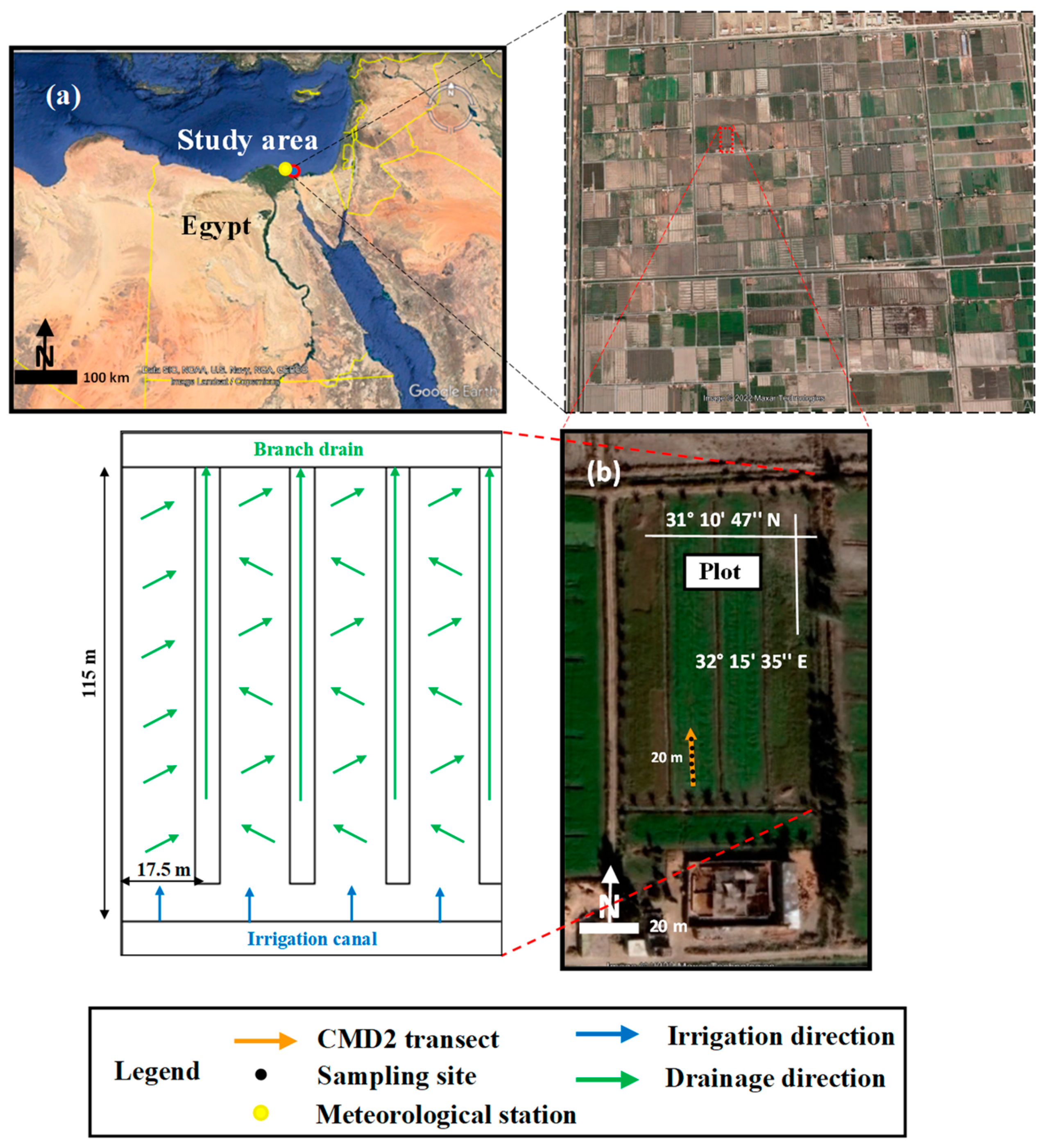
2.1. Study Area

The study area is located approximately 10 km south of Port Said City in Egypt (Figure 1a). This study focused on one intensely used and representative agricultural plot in the area, as shown in Figure 1b. The Suez Canal bounds this area to the east and El-Manzala Lake to the west. The area is located between 32°15′ E to 32°17′ E longitude and 31°10′ N to 31°11′ N latitude, covering an agricultural area of 1200 ha. This area has a relatively flat topography, with an elevation ranging from 1 to 2 m above the mean sea level. The soil texture in the study area is classified as sandy clay loam [33], and the region is classified as arid according to the Köppen–Geiger climate classification [34]. In the past, this area was part of Lake Manzala but was drained and converted into agricultural land in 1990, where sabkha deposits and salt crusts with remnants of seashells dominate the region. When the water was drained from the lake, it left behind a sediment layer that was rich in nutrients and organics. However, the sediment layer also contains high levels of salt, which can lead to soil salinization and decreased crop productivity over time [35].
The plot comprises four basins, and the dimensions of each basin, as well as the location of the drainage water and irrigation water system, are depicted in Figure 1b. Figure 2 displays daily recordings of the total rainfall and average temperature obtained throughout the study period at the Port Said meteorological station, indicated by the yellow circle in Figure 1a, located at 31°15′36.0″ N and 32°17′24.0″ E, along with irrigation and survey events [36]. The average annual rainfall is 98 mm, mainly occurring in winter with a maximum amount of 49 mm in January. The average minimum and maximum temperatures are 4.2 and 42.6 °C, occurring in January and May, respectively. The groundwater level was measured during each survey and the recorded depth was similar and approximately around 0.85 m during all surveys.
Flood irrigation is the main irrigation method used in the study area. The agricultural plot receives irrigation water from the final branch of the Port Said Canal, which receives its water supply from the Ismailia Canal. The irrigation canal used to irrigate the agricultural lands in the study area is part of the national canal rehabilitation project initiated by the Egyptian Government [37]. This canal was recently lined with cement concrete during the period between January 2022 and May 2023. During the 2021 surveys, there was occasional seepage of drainage water into the canals due to the absence of canal lining. Before the lining, the measured electrical conductivity of the irrigation water (ECw) was 4.0 dS m−1, falling within the moderately saline range (2–10 dS m−1) as defined by FAO guidelines [38]. However, according to the guidelines for interpretations of water quality for irrigation, which take into account crop tolerance to salinity, the degree of restriction is severe for use with ECw values superior to 3 dS m−1 [39]. Following the initiation of canal lining, subsequent measurements indicated a significant reduction in the ECw, decreasing to 1 dS m−1 which falls within the slightly saline range (0.7–2 dS m−1). The surface drainage system consists of open drains in a V-shaped pattern with a depth of 1.0 m and which are 17.5 m apart. These drains ultimately converge into the branch drain, as shown in Figure 1b.
The main crop cultivated in the area is Sorghum Sudanese (Sorghum bicolor subsp. drummondii), which is used as animal feed. The geophysical surveys were conducted to monitor the soil salinity of the investigated plot at the 20 m transect shown in Figure 1b. These surveys mainly aimed to track the temporal variation in soil salinity distribution during a complete agricultural season. The salinity levels in the plot were relatively moderate, with vegetation covering the entire plot. The Turkmen Agricultural Institute found that planting Sorghum Sudanese in saline areas reduces soil salinity, promoting healthy crop growth and yields [40]. Additionally, it lowers the groundwater level and prevents soil salinization [40,41]. The productivity of Sorghum Sudanese has the potential for up to five annual harvests [42]. The study area was initially prepared for planting Sorghum Sudanese in September 2021 when fertilization with potassium, nitrogen, and phosphate, as well as seed sowing, were conducted. However, the presence of harmful weeds caused a delay in cultivation until December 2021. The cultivation extended over six months, encompassing five harvests, with the last harvest in May 2022.

2.2. Soil Sampling and Laboratory Analysis

As shown in Figure 1b, soil samples were taken along the investigated transect on all dates concurrently with EMI surveys. Between 1 and 6 boreholes were drilled, depending on the date of measurement, as illustrated in Table 1. At each borehole location, three soil samples were collected along a 90 cm depth representing topsoil (0.0–0.3 m), subsurface (0.3–0.6 m), and subsoil (0.6–0.9 m). The ECe of the soil saturation paste extract was determined in the soil laboratory of the Faculty of Engineering, Port Said University, Egypt. The collected soil samples were air-dried at room temperature and the portion of the soil that passed through a 2.0 mm sieve was weighed and placed in a container. A volume of distilled water was added to the soil, stirring thoroughly until a saturated paste was achieved. The soil was allowed to be fully saturated by covering the container and letting it sit for 24 h. After saturation, according to Richards [43], the ECe was measured in the extract obtained using suction filters from soil saturation paste using a conductivity meter (HI5521-01). In general and according to the soil salinity classification proposed by Barrett-Lennard et al. [44], the soil was considered non-saline, slightly saline, moderately saline, highly saline, and severely saline if its ECe ranged from 0 to 2 dS m−1, 2 to 4 dS m−1, 4 to 8 dS m−1, 8 to 16 dS m−1, and >16 dS m−1, respectively.

2.3. Collection and Inversion of ECa Data

ECa data were collected using a low-frequency electromagnetic induction (EMI) technique (i.e., a CMD2 conductivity meter; GF Instruments). The CMD2 has a transmitter coil consisting of horizontal (ECah) and vertical (ECav) receiver arrays. It functions at a frequency of 10 kHz. The separation between the transmitter and receiver is 1.89 m, allowing for theoretical measurements of ECa depths ranging from 0.0 to 1.5 m and 0.0 to 3.0 m for the ECah and the ECav, respectively.
In the beginning, a pilot survey was conducted with the CMD2 positioned approximately 1.00 m above the ground surface throughout the investigated plot (Figure 1b) to explore variations in soil salinity. Only the horizontal dipole orientation was considered during this survey. The objective of the initial investigation was to gain qualitative insights into the spatial variability of soil salinity across the field and to identify a representative transect for further study. According to this survey, a specific transect within the investigated plot was selected for detailed study (Figure 1b). The location of this transect was selected based on the variability of the measured ECa values in the investigated plot (Figure 3).
Notable heterogeneity in the ECa values was observed along this transect. Furthermore, it was oriented parallel to the drainage direction, located between two drains to ensure that the CMD2 readings were not affected by drainage water or its salinity. Subsequently, a series of CMD2 surveys were conducted along the selected single transect over a period spanning six dates from August 2021 to April 2023. Measurements were obtained at intervals of 1 m along the 20 m transect (Figure 1) using a GPS integrated with the device for registration of the position. The ECa was collected with a CMD2 lying on the ground surface in both horizontal and vertical dipole orientations.
For the inversion, the EM4Soil software (V-3.05) [45] was used to estimate the true electrical conductivity (σ, mS m−1) at any depth. These estimates were generated by using 1D laterally constrained inversion, Quasi 2D, a technique developed by [16,46,47]. A forward model based on the full solution of the Maxwell equations [48] was used in this study. This method is recommended when the ECa values are high (>100 mS m−1). Two different inversion algorithms, S1 [49] and S2 [50], were used that are based on Occam regularization [51]. To run these algorithms, the special Lagrangian multiplier (λ) should be determined. λ is responsible for regulating the balance between the smoothness of the spatial model and the misfit to the data response. A larger λ typically results in a model with a greater misfit error but smoother conductivity values. This is generally acceptable when soil conductivity changes follow a gradual pattern, leading to a more realistic model. Conversely, a smaller λ is usually required when anticipating sharper transitions in soil conductivity to accurately delineate abrupt boundaries. The determination of a suitable λ value is typically conducted through inversions with various λ values [52,53].
The number and depth of layers in the initial model and the conductivities of each layer were determined based on the ECa data mean. The value of λ varied from 0.02 to a maximum of 3.0, with inversion stopping after a maximum of 10 iterations.
Two different techniques were used to invert the six surveys, namely individual and time-lapse inversion. In the individual inversion, each survey was inverted independently, and only spatial regularization was applied. In contrast, in the time-lapse inversion, the data for the six dates were simultaneously inverted and the temporal regularizations were also applied. Therefore, it was necessary to optimize the spatial and temporal Lagrangian multipliers. The temporal Lagrangian multiplier (α) functions as a temporal damping factor, assigning weight to the minimization of temporal conductivity changes along the time axis. The α remains constant and is determined by the similarity between two consecutive reference times. A higher α value yields more similar reference models resulting from the inversion, while a value of zero signifies the absence of temporal constraints, resembling a traditional non-time-lapse inversion [54].
The value of λ used in the current study ranged from 0.02 to a maximum of 1.5, while α was set at either 0.5 or 0.1, with a maximum number of 10 iterations. To develop optimum electromagnetic conductivity images (EMCIs) relative to the measured ECe, the CMD2 ECa data associated with the soil sampling sites were used. Subsequently, the optimal inversion method was determined based on whether the individual or time-lapse inversion algorithm provided a better LR for the soil salinity calibration and optimal inversion parameters were chosen. The selected parameters achieved a higher R2 value between σ and the measured ECe and a lower model misfit error among different regression models (EMCIs). The R2 values were compared using the classification proposed by Moore and Kirkland [55], where a strong agreement was defined as R2 > 0.70, moderate as 0.5 < R2 < 0.7, weak as 0.3 < R2 < 0.5, and very weak as R2 < 0.3.

2.4. Prediction of ECe from EMCI Using Site-Specific Calibrations

As a first step, a unique equation (i.e., a site-specific calibration equation) was derived for the investigated plot based only on the ECa data from the third survey. The best-selected sets of inversion parameters described in Section 2.3 were used to develop a linear regression model between σ and the measured ECe.
After that, a cross-validation process was used to assess the predictive ability of the calibration equation. Cross-validation was carried out using the leave-one-out cross-validation (LOOCV; [56]) method. In this method, one sample was removed, and the calibration was established based on the remaining samples to predict the ECe at the point where the sample was removed. This process was iteratively repeated for each sampling point from the sampling sites (18 soil sampling points) until each sample had been taken once. The ability of the site-specific calibration to predict the ECe was assessed using several metrics. The root mean square error (RMSE; Equation (1)) was computed to evaluate the overall prediction accuracy and the mean error (ME; Equation (2)) was calculated to assess any prediction bias. Additionally, Lin’s concordance correlation coefficient (LCCC; [57]) was calculated to evaluate the degree of similarity between the linear regression (LR) and the 1:1 relationship and to quantify the agreement between the two variables.
R M S E = 1 n j = 1 n E C p i E C m i 2
M E = 1 n j = 1 n E C m i E C p i
where n is the total number of data points; ECmi and ECpi are the measured and predicted ECe values, respectively.
In the second step, repeated EMI and ECe measurements, which were collected simultaneously with the EMI surveys for all measurement surveys except survey 3, were used as an independent validation dataset. This dataset was employed to assess (i.e., validate) the prediction ability of the site-specific calibration to predict ECe values from EMCIs at various depths over time. This was performed for both inversion techniques (i.e., time-lapse and individual inversions).
In the last step, the RMSE, ME, and LCCC were used as indicators to evaluate the ability of the site-specific calibration equation to predict the ECe.

3. Results

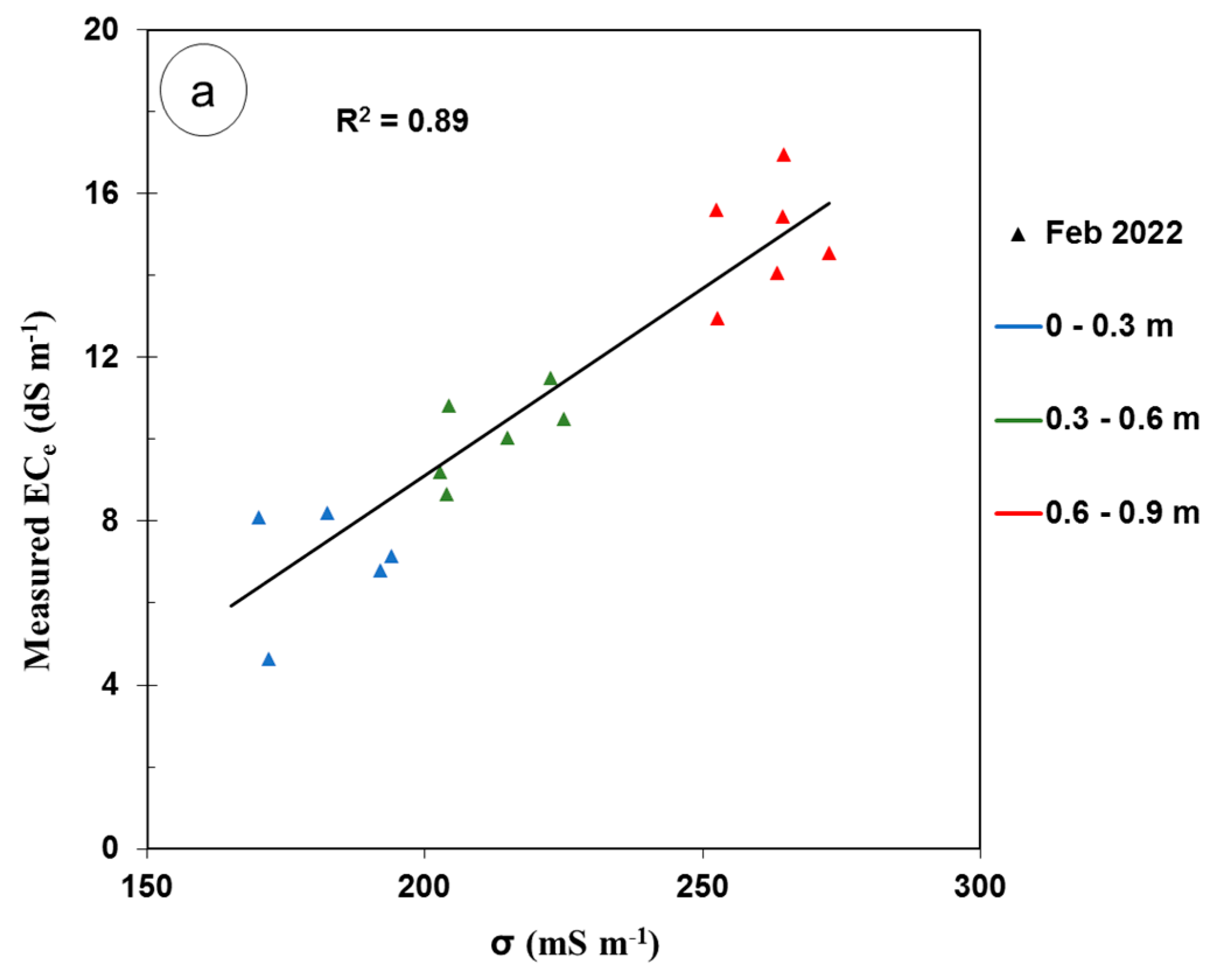
3.1. ECe Data Analysis

Initially, the third survey was chosen as a calibration dataset based on the fact that this survey included both the minimum and maximum ECe values measured across all surveys (Table 2) and it had a wide range of ECe values (ECe range = 12.32 dS m−1). Moreover, the third survey was characterized by the largest number of soil samples collected during the surveys (i.e., n = 18). Table 3 summarizes descriptive statistics for the measured ECe values in the calibration dataset (i.e., n = 18; the third survey). In the first layer (0.0–0.3 m), the minimum ECe value was 4.63 dS m−1, which is classified as moderately saline (4–8 dS m−1). Both the mean (7.16 dS m−1) and the maximum (8.19 dS m−1) ECe values showed moderate and high salinity levels, respectively. The ECe in the second layer (0.3–0.6 m) was highly saline (8–16 dS m−1), with a minimum ECe value of 8.66 dS m−1, a maximum of 11.50 dS m−1, and a mean of 9.96 dS m−1. In the third layer (0.6–0.9 m), the minimum ECe value was 12.95 dS m−1 and the mean was 14.92 dS m−1, indicating high salinity, while the maximum ECe value was 16.95 dS m−1, which is classified as severely saline (16–32 dS m−1).
Table 3 summarizes the statistics of the measured ECe in the validation dataset (i.e., n = 57). In the first layer, the minimum and the mean ECe values were 5.29 and 7.47 dS m−1, respectively, and was moderately saline, while the maximum ECe value was 11.8 dS m−1 and was highly saline. In the second layer, the validation ECe data had minimum, mean, and maximum ECe values of 8.00, 10.89, and 12.59 dS m−1, respectively. These values were slightly higher than the calibration data, except for the minimum. The validation ECe data for the third layer demonstrated lower minimum, mean, and maximum values in comparison to the calibration dataset.
The statistics for all layers in the calibration samples fell within the same salinity classes, with only a difference in the maximum value of the third layer. This high level of consistency enhances confidence in the calibration model’s ability to provide accurate estimations for ECe values.
By comparing the calibration and the validation datasets, it can be noted that the mean ECe value (i.e., 10.68 dS m−1) was slightly higher for the calibration dataset. The standard deviation (SD) was also slightly higher for the calibration ECe dataset and was equal to 3.52 dS m−1 as compared to 2.94 dS m−1 corresponding to the validation ECe dataset, indicating greater variability in the calibration ECe data. Both the minimum and the maximum values were slightly higher for the calibration ECe dataset. Furthermore, the coefficient of variation (CV) was higher for the calibration ECe dataset and was equal to 32.9% as compared to 27.9% for the validation ECe dataset, suggesting that the calibration ECe data exhibited relatively higher variability with their mean.

3.2. Determination of the Optimal Inversion Parameters and Inversion Technique

After the analysis of determining the optimal parameter configuration for individual inversion and establishing a calibration relationship between σ and the measured ECe, the best sets of inversion parameters were assessed. These were obtained using the S2 inversion algorithm, FS forward modeling, and λ = 0.4. The calibration equation developed from the individual inversion was as follows with an R2 value of 0.88:
ECe = 0.3084 + 0.05039 × σ
Likewise, to determine the optimal parameter configuration for time-lapse inversion and to develop a calibration relationship between σ and the measured ECe, various EMCIs were generated. These were created by using ECa data from all EMI survey dates; employing inversion algorithms (S1 and S2); and varying the initial model conductivity, λ, and α values as described in Section 2.3.
Firstly, it is worth mentioning that the model derived using λ values exceeding one is not shown here. Using λ values higher than one led to a considerable misfit error between the predicted and measured ECa. Therefore, opting for a high λ is not advisable, especially when expecting sharp vertical conductivity contrasts in the field. Regarding the impact of the temporal smoothing parameter (α), various values were investigated (results not presented here). It was observed that values exceeding 0.10 overly smoothed the anticipated temporal changes, making it challenging to resolve detailed variations. Hence, for this study, a value of 0.10 was determined to be the optimal choice for α in addressing the temporal variation of σ.
An analysis for the time-lapse inversion technique was conducted using the best-selected sets of inversion parameters. These parameters were achieved when using the S2 inversion algorithm, α = 0.10, and λ = 0.90. The calibration equation developed from TL inversion was as follows with an R2 value of 0.89:
ECe = −9.1485 + 0.0910 × σ
Table 4 presents the R2 values between σ and the measured ECe for both the individual (IN) and time-lapse (TL) inversion techniques. Moreover, it shows the RMSE, ME, and LCCC between the measured and predicted ECe values for all data calculated by using site-specific calibration equations for both techniques (i.e., Equations (3) and (4)). These estimates were assessed by considering survey 3 (i.e., n = 18) as the calibration dataset and the remaining surveys (i.e., n = 57) as the validation dataset. The R2 values were strong for all surveys (i.e., R2 > 0.70) using both techniques, with R2 values of 0.81 and 0.77 for time-lapse and individual inversion, respectively. This suggests that the time-lapse technique may offer a slightly more accurate calibration for the measured ECe.
Considering the mean error (ME) between the measured and predicted ECe values for all surveys, it was clear that the least biased (i.e., closest to zero) inversion technique was the time-lapse inversion as it represented an ME value of 0.17 dS m−1 compared to 0.85 dS m−1 for the individual inversion.
According to Singh et al. [58], a satisfactory prediction RMSE should be half the standard deviation (SD) of the measured ECe. As the SD of the ECe for all the validation data was 2.94 dS m−1, as shown in Table 3, the RMSE should be 1.47 dS m−1 or lower to achieve satisfactory prediction. As the RMSE was equal to 1.45 dS m−1 in the time-lapse inversion as compared to 2.10 dS m−1 in the individual inversion, the time-lapse inversion is considered the optimal inversion technique.
The LCCC between the measured and predicted ECe values for all surveys is displayed in Table 4. The analysis of the LCCC reinforced the superiority of the time-lapse inversion technique, with a stronger agreement between the measured and predicted ECe (LCCC = 0.90) compared to that in the individual inversion (LCCC = 0.84), indicating the effectiveness of time-lapse inversion in making predictions. Based on the results, time-lapse inversion is recommended compared to individual inversion as it showed improved accuracy and effectiveness in ECe prediction. Therefore, the time-lapse inversion technique was applied in this study and used for monitoring and mapping soil salinity, as shown below.

3.3. Time-Lapse EMCIs

Figure 4 displays the obtained EMCIs from the time-lapse inversion of EMI surveys. The figure shows that σ increases with depth, consistent with the previously established soil salinity distribution. Across multiple EMI surveys conducted at the same location, the temporal variations in σ were monitored for one agricultural season spanning from August 2021 to June 2022. In August 2021, the σ values fluctuated between a minimum value of 138.4 mS m−1 and a maximum value of 352.5 mS m−1. This wide range indicated significant variability in σ compatible with the large measured ECe within this timeframe.
In September 2021, the σ values ranged from 142.7 to 343.7 mS m−1. The recorded σ ranges for both dates can be attributed to fertilizer application, irrigation water salinity (ECw = 4 dS m−1), and the existence of shallow saline groundwater with a depth level of 0.85 m below the soil surface and a salinity of 14 dS m−1. In arid climates and under evaporation, an important solute up-flow from the shallow and salty groundwater (capillarity rise processes) could be the main cause of soil salinization [59].
In February 2022, the maximum σ values decreased compared to those in August and September 2021. The σ values in February 2022 ranged from 142.7 to 323.7 mS m−1. April 2022 exhibited a similar pattern, with σ values ranging from 145.4 to 318.1 mS m−1. This reduction in the maximum σ values can be attributed to the winter rains, as shown in Figure 2. This resulted in a corresponding decrease in the measured ECe which agreed with the reduction in σ values in the subsoil, as shown in Figure 4. In June 2022, a slight increase in the minimum σ values was noted and the σ values ranged from 152.17 to 322.21 mS m−1.
Finally, in April 2023, another agricultural season one year later, the σ values ranged from 157.0 to 329.8 mS m−1, maintaining an almost consistent pattern as observed during the antecedent four surveys. This pattern involves a decrease in σ values within the subsoil as compared to those in February 2022 as shown in Figure 4. This trend was also reflected in the measured ECe values in the subsoil. The ECe values decreased in the subsoil.

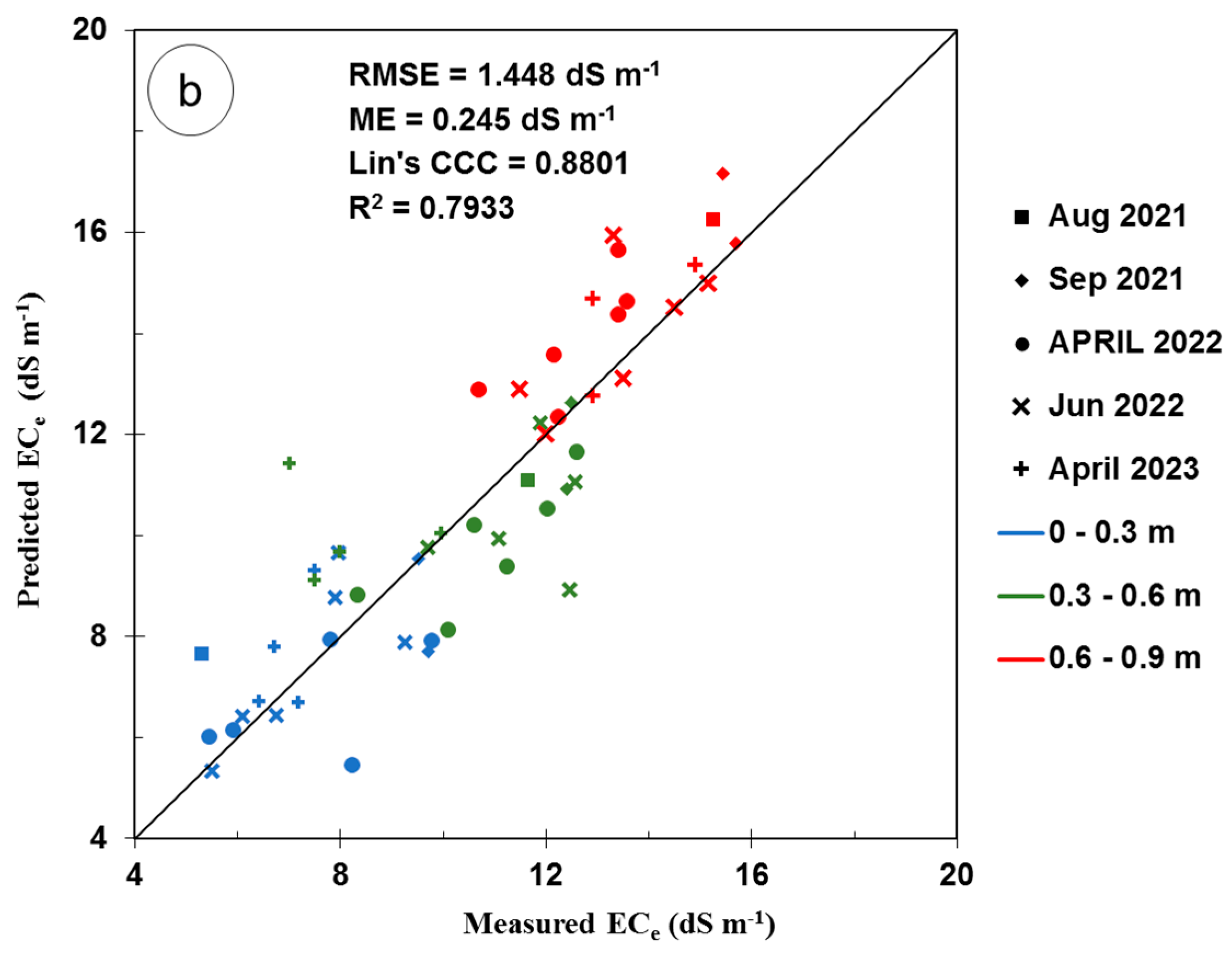
3.4. Prediction of ECe Using Site-Specific Calibration

Figure 5a displays the calibration relationship between the ECe and σ using the calibration equation developed from survey 3 using the time-lapse technique and the best inversion parameters (i.e., the S2 inversion algorithm, α = 0.10, and λ = 0.90). The best LR equation gave an R2 equal to 0.89, expressed as
ECe = −9.1485 + 0.0910 × σ
Figure 5b shows the predicted ECe plotted versus the measured ECe and the 1:1 line using the calibration equation developed using the time-lapse for different measurement dates and different measurement depths.
The validation of the calibration equation using time-lapse inversion resulted in an RMSE of 1.45 dS m−1 and a strong R2 of 0.79, indicating acceptable predictive capability given the wide ECe range (10.41 dS m−1). These results concur with the findings of Zare et al. [60], who observed a larger RMSE (5.28 dS m−1) in an irrigated cotton field under a wider ECe range (68.4 dS m−1). However, in the current study, the predictive bias (ME) was small and equal to 0.24 dS m−1, indicating a slight tendency for overestimation of the ECe. This level of bias was slightly higher than the ME reported by Zare et al. [60], which was 0.03 dS m−1. However, it can be considered well within acceptable limits. A high LCCC of 0.88 indicates a strong agreement between the measured and predicted ECe values during validation.
Figure 5b displays variations in the predictive accuracy of the validation data for all EMI survey dates. The figure shows that the predicted ECe was generally slightly overestimated in the subsoil, particularly in April 2022. This result is unsurprising, given that the soil in April 2022 had the lowest maximum measured ECe among other survey dates, as shown in Table 2. Also, these results could be explained by the spatial variation in the soil properties (such as the soil texture and cation exchange capacity) and the temporal spatial variation in the soil water content and shallow ground water properties (depth and salinity).
In contrast, the predicted ECe in the subsurface was generally slightly underestimated except for that in April 2023. This discrepancy is likely due to April 2023 having the lowest ECe among other survey dates. The greater variations in the measured ECe values during survey 3 had a considerable impact on the calibration equation, limiting its ability to monitor the smaller variations observed in April 2022 and 2023. For the topsoil layer across all observation dates, the data points exhibit a dispersed distribution around the unity line (Figure 5b).
Generally, the statistical indicators presented in Table 4 for the validation data, segregated by measurement date, indicate that the prediction ability remained relatively consistent across all five dates. These results indicate that the spatial variability of the data had a much stronger influence on the prediction ability of the site calibration than the temporal variability. To improve the spatial sensitivity of the site calibration, observation times can be extended, the number of EMI surveys can be also increased, and a different EM device with a shallow effective depth, like the CMD mini explorer, can be used. Paz et al. [9] recommended soil sampling and continuous monitoring of the volumetric water content (θ), soil temperature, groundwater level, and salinity to improve the spatial sensitivity of the site calibration.

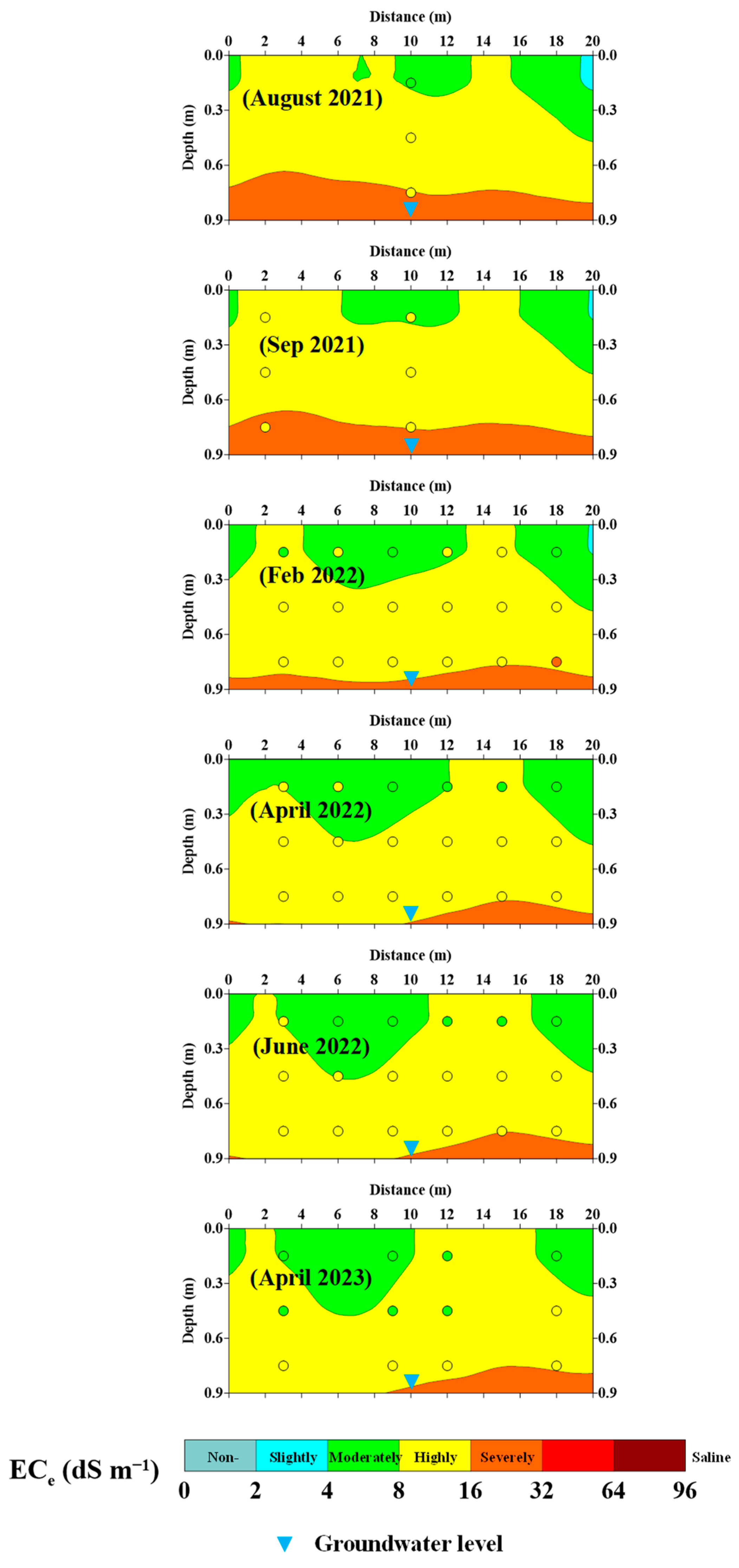
3.5. Generation of Soil Salinity Cross-Sections from Time-Lapse EMC

Figure 6 shows the soil salinity cross-sections for each EMI survey date. Consequently, the figure tracks the salinity dynamics over time. The cross-sections were generated by using the site-specific calibration equation to predict the ECe, which was classified into three salinity classes ranging from moderately to severely saline. The measured ECe values for each EMI survey’s sampling site and groundwater level are also displayed.
Furthermore, the elevated ECgr reached a high saline level of 14 dS m−1 during the dry period of the year (i.e., the summer of 2021). Higher groundwater salinity levels can be attributed to the absence of rainfall and the use of moderately saline irrigation water. However, the degree of salinity overestimation tended to subside during the winter surveys, due to rainfall which reduced the groundwater salinity to a relatively lower level (ECgr = 10 dS m−1). Figure 6 depicts soil salinity fluctuations for all surveyed dates. The soil salinity at the subsurface layer was accurately predicted in most sampling sites on all dates. In contrast, soil salinity predictions for the topsoil tended to be slightly overestimated.
During September 2021, the salinity cross-section revealed a larger portion of high salinity within the topsoil layer. In February and April 2022, many soil sample sites reached a moderately saline level as indicated by the measured ECe. In April 2023, the measured ECe at all sampling sites within the top and the subsurface soils showed a moderate saline level (ECe = 4–8 dS m−1). However, the salinity cross-sections for the topsoil estimated by CMD2 did not accurately reveal changes in soil salinity and tended to be overestimated. This inconsistency may be attributed to the weak correlation between the responses of the CMD2 device and the topsoil layer, as demonstrated in similar results obtained with an EMI device with an effective depth of 2.0 m [61]. The CMD2 has an effective depth of 1.5 m for horizontal (ECah) and 3 m for vertical (ECav) receiver arrays according to the manufacturer’s guide. This exploration depth was significantly larger than the depth of the topsoil, which makes it challenging to resolve ECe changes in the topsoil [62].
Considering the circumstances of elevated initial soil salinity, active water movement, salt conveyance, and the presence of a shallow groundwater table, salts migrated upward through capillary action and accumulated within the root zone. This phenomenon was particularly notable during the dry season of summer 2021. However, the use of slightly saline irrigation water (after canal lining) led to a gradual reduction in soil salinity, particularly within the topsoil, proven by subsequent EMI survey dates.
Using the information obtained from time-lapse spatial distribution maps, the classification of soil salinity becomes a valuable tool for rational crop allocation within the investigated agricultural field. The primary objective of this allocation strategy is to effectively maximize crop yield in salt-affected soils. This approach involves the cultivation of crops renowned for their high salt tolerance, such as cotton, barley, and sorghum, even in soils exhibiting moderate to heavy salinity levels. The results of the current study can help local farmers monitor soil salinity more accurately, allowing them to develop customized soil management strategies and make informed decisions in agriculture.

4. Discussions

It is worth noting that the minimum ECe at all depths, excluding the topsoil, indicated highly saline conditions. The higher salinity values in the study area can be attributed to climate change, leading to sea-level rise [63,64]. Consequently, this phenomenon impacts the groundwater, causing an increase in saltwater intrusion from El Manzala Lake, located near the study area [65]. Although Sorghum Sudanese is generally moderately salt-tolerant, the grain yields of two cultivations decreased by 16% per unit increase in ECe values above 6.8 dS m−1 [66]. Sorghum is soil- and water-salinity tolerant up to 6.8 and 4.5 dS m−1, respectively [67], in the investigated agricultural field. The crop yield was high, which is consistent with the results of Almodares and Sharif [68]. Additionally, the extended trials conducted at the Turkmen Agricultural Institute demonstrated the feasibility of achieving a substantial Sorghum Sudanese yield, even in the presence of highly saline soils [40]. A higher Sorghum Sudanese yield in the investigated plot can also be attributed to the use of organic and mineral fertilizers during the cultivation season.
The reduction in σ and measured ECe values within the subsoil can be attributed to the decrease in irrigation water salinity due to the canal lining and the continued cultivation of Sudanese Sorghum. Although the decrease in irrigation water salinity resulted in a reduction in measured ECe within the topsoil layer during the last survey, no corresponding decrease was observed in σ. This can be attributed to the lower sensitivity of the CMD2 to soil salinity within the root zone due to the existence of shallow groundwater which considerably affects the readings and the high temporal variation in soil moisture at the topsoil under evapotranspiration demand and water apply events [6]. Also, according to McNeill [69], part of the salts present in surface soils may not be in solution due to low water contents and therefore will not affect the CMD2 readings. Moreover, a smoothness constraint was imposed in the modeling to stabilize the inversion and smooth conductivity variations over short depth increments [54,70]. Consequently, the ability to predict salinity from σ in the topsoil was diminished, as discussed earlier in Section 3.5. To improve the prediction of soil salinity in topsoil, other EMI multi-coil sensors such as the CMD Mini Explorer can be used. These sensors are designed for detailed investigation of the topsoil as they feature multiple receivers situated closely to the transmitter, thus providing more detailed ECa data for the topsoil. In the absence of such a sensor, multi-height ECa measurements [71] might also help to better resolve topsoil conductivity variations in short depth increments. Furthermore, obtaining additional soil information, particularly related to water content and soil texture, could facilitate a more comprehensive assessment of the influence of other soil properties on the EMI signal for a more precise evaluation of topsoil salinity.
The salinity cross-sections revealed that the salinity levels tended to increase with depth, starting from a moderately saline level in the topsoil to a highly saline level in the subsoil. Severe saline zones were found at the bottom of the subsoil layer across every surveyed date. These saline zones overestimated soil salinity compared to the measured ECe values. The observed overestimation can be attributed to the proximity of groundwater to the root zone. Shallow groundwater can affect CMD2 measurements because water is a significantly better conductor of electricity than soil. Consequently, this situation can lead to an overestimation of soil salinity.
The increase in salinity at the topsoil layer during September 2021 can be primarily attributed to the application of fertigation practices and the use of saline irrigation water (ECw of 4.0 dS m−1). Subsequently, with the arrival of the winter and rainy seasons, which represented 66% of the year 2021’s total annual rainfall, the salinity levels decreased. It is worth mentioning that the initiation of canal lining in January 2022 led to a considerable reduction in irrigation water salinity. The salinity of irrigation water decreased to 1.0 dS m−1 by April 2023. This reduction in water salinity notably contributed to lower soil salinity levels.
The adoption of Sorghum Sudanese cultivation may be another factor for soil salinity reduction during the successive surveys. Worku et al. [72] investigated the effect of Sudanese Sorghum cultivation for eighteen months on the changes in soil ECe. The results showed a remarkable improvement in soil salinity with a reduction in ECe of 52.60% (from 9.81 to 4.65 dS m−1) in the upper 0–30 cm soil layer and of 54.76% (from 7.67 to 3.47 dS m−1) in the lower 30–60 cm. Mirsharipova et al. [42] stated that Sorghum Sudanese can absorb salts from the soil and thereby decrease the soil salinity. The yield of Sorghum Sudanese in the investigated agricultural plot increased by more than 10% during the year 2023, which can be attributed to the reduction in soil salinity.
Challenges in generating soil-salinity predictive maps at the field-scale were faced due to the following reasons: (i) a lack of repeated field-scale EMI surveys across the entire field and only having data from a single measurement; (ii) the absence of soil sample collection on the day of the field-scale EMI survey, preventing the upscaling of our approach for predictive maps, even on that single day; and (iii) limited EMI measurements in a single orientation during the field-scale investigation, rendering them unsuitable for the inversion modeling that was presented for quantitative investigation.

5. Conclusions

This study employed EMI surveys and soil sampling to estimate soil salinity distribution across a 20 m transect within a highly utilized agricultural plot in the risk-prone Port Said region, Egypt. Through time-lapse inversion and site-specific calibration, the EMI data were transformed into soil salinity cross-sections, enabling the assessment of soil salinity dynamics. The developed soil salinity cross-sections showed how soil salinity responds to inputs such as salts and water, whether through irrigation, rainfall, or changes in shallow groundwater salinity. This method can assess suitable agricultural management practices for salinity reduction. Notably, the study revealed that cultivating Sudanese Sorghum contributed to a reduction in soil salinity, while canal lining also played a role in lowering soil salinity due to its direct impact on ECw.
The outlined methodology showcased reliable predictions of soil salinity over time, underscoring the suitability of the CMD2 device for monitoring soil salinity. However, it revealed a limitation in accuracy for the topsoil layer (0–0.3 m). This limitation is primarily attributed to the CMD2’s lack of resolution for topsoil characterization, compounded by the substantial variability of other soil properties, notably water content. The latter significantly impact the EMI signal and soil salinity assessment. To address this limitation and enhance topsoil salinity monitoring, the use of sensors specifically designed for shallow investigations, such as the CMD Mini Explorer, is recommended.
Addressing irrigation water and soil salinity management challenges is often complex, particularly in fields and at large scales. The EMI method offers a non-invasive, rapid, and cost-effective solution for soil salinity dynamic monitoring that can cover expansive areas quickly. Although our study focused on a small transect, there is potential for scaling up from small-scale to field assessments due to the method’s ability for rapid data collection. Our attempt is now towards securing additional funding to facilitate this undertaking in the near future. It is important to highlight that such applications have been very rare in Egypt, despite many lands facing issues with soil salinity and degradation. We consider this study as a proof of concept to demonstrate how EMI can be applied in this region for quantitative monitoring of soil salinity. This lays the foundation for further research to explore the efficacy of EMI sensors and incorporate them into broader 4D investigations for monitoring soil salinity in fields and at large scales.

Author Contributions

Conceptualization, M.G.E., M.F., M.E. and T.S.; Data curation, A.A. and M.F.; Formal analysis, M.G.E., A.A., M.F. and T.S.; Funding acquisition, M.G.E., M.E. and T.S.; Investigation, M.G.E., A.A. and T.S.; Methodology, M.G.E., A.A., M.F., F.B., M.E. and T.S.; Project administration, M.G.E., M.E. and T.S.; Resources, M.E. and T.S.; Software, A.A. and M.F.; Supervision, M.G.E., M.F., M.E. and T.S.; Validation, A.A. and M.F.; Visualization, M.G.E., M.F., M.E. and T.S.; Writing—original draft, A.A., M.F. and T.S.; Writing—review and editing, M.G.E., M.F., F.B., M.E. and T.S. All authors have read and agreed to the published version of the manuscript.

Funding

This research received no specific grant from any funding agency in the public, commercial, or not for profit sectors.

Data Availability Statement

Data is contained within the article.

Acknowledgments

This study was supported by the Egyptian Academy of Scientific Research and Technology through the SALTFREE project (ARIMNET2/0005/2015, Coordination of Agricultural Research in the Mediterranean Area).

Conflicts of Interest

The authors declare no conflicts of interest.

References

  1. Stavi, I.; Thevs, N.; Priori, S. Soil salinity and sodicity in drylands: A review of causes, effects, monitoring, and restoration measures. Front. Environ. Sci. 2021, 9, 330. [Google Scholar] [CrossRef]
  2. FAO. Global Symposium on Salt-Affected Soils: Outcome Document; FAO: Rome, Italy, 2022. [Google Scholar]
  3. Shrivastava, P.; Kumar, R. Soil salinity: A serious environmental issue and plant growth promoting bacteria as one of the tools for its alleviation. Saudi J. Biol. Sci. 2015, 22, 123–131. [Google Scholar] [CrossRef]
  4. Machado, R.M.A.; Serralheiro, R.P. Soil salinity: Effect on vegetable crop growth. Management practices to prevent and mitigate soil salinization. Horticulturae 2017, 3, 30. [Google Scholar] [CrossRef]
  5. Gorji, T.; Sertel, E.; Tanik, A. Monitoring soil salinity via remote sensing technology under data-scarce conditions: A case study from Turkey. Ecol. Indic. 2017, 74, 384–391. [Google Scholar] [CrossRef]
  6. Bouksila, F.; Persson, M.; Bahri, A.; Berndtsson, R. Electromagnetic induction prediction of soil salinity and groundwater properties in a Tunisian Saharan oasis. Hydrol. Sci. J. 2012, 57, 1473–1486. [Google Scholar] [CrossRef]
  7. Li, X.-M.; Yang, J.-S.; Liu, M.-X.; Liu, G.-M.; Yu, M. Spatio-temporal changes of soil salinity in arid areas of south Xinjiang using electromagnetic induction. J. Integr. Agric. 2012, 11, 1365–1376. [Google Scholar] [CrossRef]
  8. Li, H.; Shi, Z.; Webster, R.; Triantafilis, J. Mapping the three-dimensional variation of soil salinity in a rice-paddy soil. Geoderma 2013, 195, 31–41. [Google Scholar] [CrossRef]
  9. Li, H.; Webster, R.; Shi, Z. Mapping soil salinity in the Yangtze delta: REML and universal kriging (E-BLUP) revisited. Geoderma 2015, 237, 71–77. [Google Scholar] [CrossRef]
  10. Paz, M.C.; Farzamian, M.; Paz, A.M.; Castanheira, N.L.; Gonçalves, M.C.; Santos, F.M. Assessing soil salinity dynamics using time-lapse electromagnetic conductivity imaging. Soil 2020, 6, 499–511. [Google Scholar] [CrossRef]
  11. Akça, E.; Aydin, M.; Kapur, S.; Kume, T.; Nagano, T.; Watanabe, T.; Çilek, A.; Zorlu, K. Long-term monitoring of soil salinity in a semi-arid environment of Turkey. Catena 2020, 193, 104614. [Google Scholar] [CrossRef]
  12. Visconti, F.; De Paz, J.M. A semi-empirical model to predict the EM38 electromagnetic induction measurements of soils from basic ground properties. Eur. J. Soil Sci. 2021, 72, 720–738. [Google Scholar] [CrossRef]
  13. Visconti, F.; de Paz, J.M. Sensitivity of soil electromagnetic induction measurements to salinity, water content, clay, organic matter, and bulk density. Precis. Agric. 2021, 22, 1559–1577. [Google Scholar] [CrossRef]
  14. Petsetidi, P.A.; Kargas, G. Assessment and Mapping of Soil Salinity Using the EM38 and EM38MK2 Sensors: A Focus on the Modeling Approaches. Land 2023, 12, 1932. [Google Scholar] [CrossRef]
  15. Auken, E.; Christiansen, A.V.; Kirkegaard, C.; Fiandaca, G.; Schamper, C.; Behroozmand, A.A.; Binley, A.; Nielsen, E.; Effersø, F.; Christensen, N.B. An overview of a highly versatile forward and stable inverse algorithm for airborne, ground-based, and bore-hole electromagnetic and electric data. Explor. Geophys. 2015, 46, 223–235. [Google Scholar] [CrossRef]
  16. Santos, F.A.M. 1-D laterally constrained inversion of EM34 profiling data. J. Appl. Geophys. 2004, 56, 123–134. [Google Scholar] [CrossRef]
  17. Dakak, H.; Huang, J.; Zouahri, A.; Douaik, A.; Triantafilis, J. Mapping soil salinity in 3-dimensions using an EM38 and EM4Soil inversion modelling at the reconnaissance scale in central Morocco. Soil Use Manag. 2017, 33, 553–567. [Google Scholar] [CrossRef]
  18. Corwin, D.L.; Yemoto, K. Measurement of soil salinity: Electrical conductivity and total dissolved solids. Soil Sci. Soc. Am. J. 2019, 83, 1–2. [Google Scholar] [CrossRef]
  19. Wang, F.; Yang, S.; Wei, Y.; Shi, Q.; Ding, J. Characterizing soil salinity at multiple depth using electromagnetic induction and remote sensing data with random forests: A case study in Tarim River Basin of southern Xinjiang, China. Sci. Total Environ. 2021, 754, 142030. [Google Scholar] [CrossRef]
  20. Xie, W.; Yang, J.; Yao, R.; Wang, X. Spatial and temporal variability of soil salinity in the Yangtze River estuary using electromagnetic induction. Remote Sens. 2021, 13, 1875. [Google Scholar] [CrossRef]
  21. Gómez Flores, J.L.; Ramos Rodríguez, M.; González Jiménez, A.; Farzamian, M.; Herencia Galán, J.F.; Salvatierra Bellido, B.; Cermeño Sacristan, P.; Vanderlinden, K. Depth-Specific Soil Electrical Conductivity and NDVI Elucidate Salinity Effects on Crop Development in Reclaimed Marsh Soils. Remote Sens. 2022, 14, 3389. [Google Scholar] [CrossRef]
  22. Khongnawang, T.; Zare, E.; Srihabun, P.; Khunthong, I.; Triantafilis, J. Digital soil mapping of soil salinity using EM38 and quasi-3d modelling software (EM4Soil). Soil Use Manag. 2022, 38, 277–291. [Google Scholar] [CrossRef]
  23. Brogi, C.; Huisman, J.; Pätzold, S.; Von Hebel, C.; Weihermüller, L.; Kaufmann, M.; Van Der Kruk, J.; Vereecken, H. Large-scale soil mapping using multi-configuration EMI and supervised image classification. Geoderma 2019, 335, 133–148. [Google Scholar] [CrossRef]
  24. Ding, J.; Yang, S.; Shi, Q.; Wei, Y.; Wang, F. Using apparent electrical conductivity as indicator for investigating potential spatial variation of soil salinity across seven oases along Tarim River in Southern Xinjiang, China. Remote Sens. 2020, 12, 2601. [Google Scholar] [CrossRef]
  25. Shi, X.; Wang, H.; Song, J.; Lv, X.; Li, W.; Li, B.; Shi, J. Impact of saline soil improvement measures on salt content in the abandonment-reclamation process. Soil Tillage Res. 2021, 208, 104867. [Google Scholar] [CrossRef]
  26. Ben Slimane, A.; Bouksila, F.; Selim, T.; Joumada, F. Soil salinity assessment using electromagnetic induction method in a semi-arid environment—A case study in Tunisia. Arab. J. Geosci. 2022, 15, 1031. [Google Scholar] [CrossRef]
  27. Utili, S. Monitoring of earthen long linear embankments by geophysical tools integrated with geotechnical probes. In Proceedings of the E3S Web of Conferences, Lisbon, Portugal, 24–26 June 2020; p. 01031. [Google Scholar]
  28. Apostolopoulos, G.; Kapetanios, A. Geophysical investigation, in a regional and local mode, at Thorikos Valley, Attica, Greece, trying to answer archaeological questions. Archaeol. Prospect. 2021, 28, 435–452. [Google Scholar] [CrossRef]
  29. Koganti, T.; Narjary, B.; Zare, E.; Pathan, A.L.; Huang, J.; Triantafilis, J. Quantitative mapping of soil salinity using the DUA-LEM-21S instrument and EM inversion software. Land Degrad. Dev. 2018, 29, 1768–1781. [Google Scholar] [CrossRef]
  30. Yao, R.; Yang, J.; Wu, D.; Xie, W.; Gao, P.; Jin, W. Digital mapping of soil salinity and crop yield across a coastal agricultural landscape using repeated electromagnetic induction (EMI) surveys. PLoS ONE 2016, 11, e0153377. [Google Scholar] [CrossRef]
  31. Yao, R.; Yang, J. Quantitative evaluation of soil salinity and its spatial distribution using electromagnetic induction method. Agric. Water Manag. 2010, 97, 1961–1970. [Google Scholar] [CrossRef]
  32. Corwin, D.; Scudiero, E. Review of soil salinity assessment for agriculture across multiple scales using proximal and/or remote sensors. Adv. Agron. 2019, 158, 1–130. [Google Scholar]
  33. USDA. Soil survey manual. In Soil Survey Division Staff; Soil Conservation Service Volume Handbook 18; U.S. Department of Agriculture: Washington, DC, USA, 2017; Chapter 3. [Google Scholar]
  34. Geiger, R. Classification of Climates after W. Köppen. Landolt-Börnstein-Zahlenwerte und Funktionen aus Physik, Chemie, Astronomie, Geophysik und Technik, alte Serie; Springer: Berlin/Heidelberg, Germany, 1954; pp. 603–607. [Google Scholar]
  35. Aziz, A.; Berndtsson, R.; Attia, T.; Hamed, Y.; Selim, T. Noninvasive Monitoring of Subsurface Soil Conditions to Evaluate the Efficacy of Mole Drain in Heavy Clay Soils. Water 2022, 15, 110. [Google Scholar] [CrossRef]
  36. Available online: https://en.tutiempo.net/ (accessed on 6 October 2023).
  37. Between Clay and Cement: Is Egypt’s Canal Lining a Solution or Dilemma for Farmers? Available online: https://infonile.org/en/2023/01/is-egypts-canal-lining-a-solution-or-dilemma-for-farmers/ (accessed on 11 September 2023).
  38. Rhoades, J.; Kandiah, A.; Mashali, A. The Use of Saline Waters for Crop Production-FAO Irrigation and Drainage Paper 48; FAO: Rome, Italy, 1992; p. 133. [Google Scholar]
  39. Ayers, R.S.; Westcot, D.W. Water Quality for Agriculture; Food and Agriculture Organization of the United Nations: Rome, Italy, 1985; Volume 29. [Google Scholar]
  40. Yollybayev, A.; Gurbanov, A. Cultivation of Sorghum and Sudan Grass on Saline Areas. Available online: https://tohi.edu.tm/usuly-gollanma/en/file/21.pdf (accessed on 10 November 2023).
  41. Clark, A. Managing Cover Crops Profitably; Diane Publishing: Darby, PA, USA, 2008. [Google Scholar]
  42. Mirsharipova, G.; Mustafakulov, D. Planting rate of Sudan grass photosynthetic activity and dependence on the period of harvest. In Proceedings of the IOP Conference Series: Earth and Environmental Science, Online, 13–16 October 2023; p. 012062. [Google Scholar]
  43. Richards, L.A. Diagnosis and Improvement of Saline and Alkali Soils; US Government Printing Office: Washington, DC, USA, 1954.
  44. Barrett-Lennard, E.; Bennett, S.J.; Colmer, T. Standardising terminology for describing the level of salinity in soils in Australia. In Proceedings of the 2nd International Salinity Forum: Salinity, Water and Society: Global Issues, Local Action, Adelaide, Australia, 31 March–3 April 2005. [Google Scholar]
  45. EMTOMO. EMTOMO Manual for EM4Soil, A Program for 1-D Laterally Constrained Inversion of EM Data; EMTOMO: Lisbon, Portugal, 2018. [Google Scholar]
  46. Monteiro Santos, F.; Triantafilis, J.; Bruzgulis, K.; Roe, J. Inversion of multiconfiguration electromagnetic (DUALEM-421) profiling data using a one-dimensional laterally constrained algorithm. Vadose Zone J. VZJ 2010, 9, 117–125. [Google Scholar] [CrossRef]
  47. Monteiro Santos, F.A.; Triantafilis, J.; Bruzgulis, K. A spatially constrained 1D inversion algorithm for quasi-3D conductivity imaging: Application to DUALEM-421 data collected in a riverine plain. Geophysics 2011, 76, B43–B53. [Google Scholar] [CrossRef]
  48. Kaufman, A.A.; Keller, G.V. Frequency and transient soundings methods in geochemistry and geophysics. Geophys. J. Int. 1983, 77, 935–937. [Google Scholar] [CrossRef]
  49. Sasaki, Y. Two-dimensional joint inversion of magnetotelluric and dipole-dipole resistivity data. Geophysics 1989, 54, 254–262. [Google Scholar] [CrossRef]
  50. Sasaki, Y. Full 3-D inversion of electromagnetic data on PC. J. Appl. Geophys. 2001, 46, 45–54. [Google Scholar] [CrossRef]
  51. deGroot-Hedlin, C.; Constable, S. Occam’s inversion to generate smooth, two-dimensional models from magnetotelluric data. Geophysics 1990, 55, 1613–1624. [Google Scholar] [CrossRef]
  52. Triantafilis, J.; Santos, F.M. Electromagnetic conductivity imaging (EMCI) of soil using a DUALEM-421 and inversion modelling software (EM4Soil). Geoderma 2013, 211, 28–38. [Google Scholar] [CrossRef]
  53. Zare, E.; Li, N.; Khongnawang, T.; Farzamian, M.; Triantafilis, J. Identifying Potential Leakage Zones in an Irrigation Supply Channel by Mapping Soil Properties Using Electromagnetic Induction, Inversion Modelling and a Support Vector Machine. Soil Syst. 2020, 4, 25. [Google Scholar] [CrossRef]
  54. Farzamian, M.; Autovino, D.; Basile, A.; De Mascellis, R.; Dragonetti, G.; Monteiro Santos, F.; Binley, A.; Coppola, A. Assessing the dynamics of soil salinity with time-lapse inversion of electromagnetic data guided by hydrological modelling. Hydrol. Earth Syst. Sci. 2021, 25, 1509–1527. [Google Scholar] [CrossRef]
  55. Moore, D.S.; Kirkland, S. The Basic Practice of Statistics; WH Freeman: New York, NY, USA, 2007; Volume 2. [Google Scholar]
  56. James, G.; Witten, D.; Hastie, T.; Tibshirani, R. An Introduction to Statistical Learning; Springer: Berlin/Heidelberg, Germany, 2013; Volume 112. [Google Scholar]
  57. Lawrence, I.; Lin, K. A concordance correlation coefficient to evaluate reproducibility. Biometrics 1989, 45, 255–268. [Google Scholar] [CrossRef]
  58. Singh, J.; Knapp, H.V.; Arnold, J.; Demissie, M. Hydrological modeling of the Iroquois River watershed using HSPF and SWAT 1. JAWRA J. Am. Water Resour. Assoc. 2005, 41, 343–360. [Google Scholar] [CrossRef]
  59. Bouksila, F. Sustainability of Irrigated Agriculture under Salinity Pressure—A Study in Semiarid Tunisia; Lund University Publications: Lund, Sweden, 2011. [Google Scholar]
  60. Zare, E.; Huang, J.; Santos, F.M.; Triantafilis, J. Mapping salinity in three dimensions using a DUALEM-421 and electromagnetic inversion software. Soil Sci. Soc. Am. J. 2015, 79, 1729–1740. [Google Scholar] [CrossRef]
  61. Khongnawang, T.; Zare, E.; Srihabun, P.; Triantafilis, J. Comparing electromagnetic induction instruments to map soil salinity in two-dimensional cross-sections along the Kham-rean Canal using EM inversion software. Geoderma 2020, 377, 114611. [Google Scholar] [CrossRef]
  62. Ramos, T.B.; Oliveira, A.R.; Darouich, H.; Gonçalves, M.C.; Martínez-Moreno, F.J.; Rodríguez, M.R.; Vanderlinden, K.; Farzamian, M. Field-scale assessment of soil water dynamics using distributed modeling and electromagnetic conductivity imaging. Agric. Water Manag. 2023, 288, 108472. [Google Scholar] [CrossRef]
  63. Dawoud, M.A. Design of national groundwater quality monitoring network in Egypt. Environ. Monit. Assess. 2004, 96, 99–118. [Google Scholar] [CrossRef]
  64. Salem, Z.E.; Elsaiedy, G.; ElNahrawy, A. Assessment of the groundwater quality for drinking and irrigation purposes in the Central Nile Delta Region, Egypt. In Groundwater in the Nile Delta; Springer: Berlin/Heidelberg, Germany, 2019; pp. 647–684. [Google Scholar] [CrossRef]
  65. Mabrouk, M.; Jonoski, A.; Solomatine, D.; Uhlenbrook, S. A review of seawater intrusion in the Nile Delta groundwater system–the basis for assessing impacts due to climate changes and water resources development. Hydrol. Earth Syst. Sci. Discuss. 2013, 10, 10873–10911. [Google Scholar] [CrossRef]
  66. Francois, L.E.; Donovan, T.; Maas, E.V. Salinity effects on seed yield, growth and germination of grain sorghum. Agron. J. 1984, 76, 741–744. [Google Scholar] [CrossRef]
  67. Calone, R.; Sanoubar, R.; Lambertini, C.; Speranza, M.; Vittori Antisari, L.; Vianello, G.; Barbanti, L. Salt tolerance and Na allocation in Sorghum bicolor under variable soil and water salinity. Plants 2020, 9, 561. [Google Scholar] [CrossRef]
  68. Almodares, A.; Sharif, M. Effects of irrigation water qualities on biomass and sugar contents of sugar beet and sweet sorghum cultivars. J. Environ. Biol. 2007, 28, 213–218. [Google Scholar]
  69. McNeill, J.D. Electromagnetic Terrain Conductivity Measurement at Low Induction Numbers; Technical note TN-6; Geonics Limited: Mississauga, ON, Canada, 1980. [Google Scholar]
  70. Dragonetti, G.; Farzamian, M.; Basile, A.; Monteiro Santos, F.; Coppola, A. In situ estimation of soil hydraulic and hydrodisper-sive properties by inversion of electromagnetic induction measurements and soil hydrological modeling. Hydrol. Earth Syst. Sci. 2022, 26, 5119–5136. [Google Scholar] [CrossRef]
  71. Farzamian, M.; Bouksila, F.; Paz, A.M.; Santos, F.A.; Zemin, N.; Salma, F.; Ben Slimane, A.; Selimi, T.; Triantafilis, J. Landscape-scale mapping of soil salinity with multi-height electromagnetic induction and quasi-3D inversion (Saharan Oasis, Tunisia). Agric. Water Manag. 2023, 284, 108330. [Google Scholar] [CrossRef]
  72. Worku, A.; Nekir, B.; Mamo, L.; Bekele, T. Comparative Advantage of Forage Grasses for Salt Tolerance and Ameliorative Effect under Salt Affected Soil of Amibara, Afar. Results of Natural Resources Management Research 2020. Available online: https://www.researchgate.net/publication/347468684_Comparative_Advantage_of_Forage_Grasses_for_Salt_Tolerance_and_Ameliorative_Effect_under_Salt_Affected_Soil_of_Amibara_Afar (accessed on 10 November 2023).
Figure 1. (a) Location of the study area in southern Port Said City; (b) location of the plot (CMD2 transect marked with orange lines and soil sampling sites with black dots) and location of the drainage water and irrigation water system (irrigation and drainage directions marked with blue and green lines, respectively.
Land 13 00225 g001
Figure 2. Distribution of daily rainfall (mm/day) and mean temperature (°C/day) recorded at the meteorological station located in the study area during the study period, including the dates of irrigation events, the corresponding irrigation water amounts (mm/day), and EMI survey dates.
Land 13 00225 g002
Figure 3. The spatial distribution of the apparent electrical conductivity (ECa, mS m−1) of the CMD2 data obtained from a pilot survey using the horizontal dipole (ECah) orientation at a height of 1.00 m.
Land 13 00225 g003
Figure 4. Time-lapse electromagnetic conductivity images (EMCIs) for the experimental plot.
Land 13 00225 g004
Figure 5. Plots of (a) soil electrical conductivity (σ, mS m−1), the measured electrical conductivity of the saturated soil paste extract (ECe, dS m−1), and the linear regression (LR) of the calibration equation using survey #3 and time-lapse inversion; (b) validation results of the LR calibration equation using other surveys excluding survey #3.
Land 13 00225 g005aLand 13 00225 g005b
Figure 6. Predicted soil salinity maps along vertical transects for the plot with representations of the measured ECe (in circles) and groundwater level (blue triangles) at the sampling sites located in the middle of each transect for all surveying campaigns.
Land 13 00225 g006
Table 1. Detailed information regarding the dates of measurements, agricultural state, number of drilled boreholes in each survey, and survey utilization.
CampaignDate of MeasurementState of AgricultureNumber of BoreholesSurvey Data Utilization
1stAugust 2021Before cultivation1Validation
2ndSeptember 2021After fertilization and sowing2
3rdFebruary 2022After second harvesting6Calibration
4thApril 2022After fourth harvesting6Validation
5thJune 2022After the last harvesting6
6thJune 2023One year later4
Table 2. Measured ECe values for each surveying campaign, all surveys, and validation surveys.
SurveysECe Min
(dS m−1)
ECe Max
(dS m−1)
ECe Range *Number of Soil Samples
First survey5.2915.249.953
Second survey9.5115.706.196
Third (calibration) survey4.6316.9512.3218
Fourth survey5.4513.588.1318
Fifth survey6.1015.169.0618
Sixth survey6.4014.908.5012
All surveys4.6316.9512.3275
Validation surveys (all surveys except the 3rd survey)5.2915.7010.4157
* ECe range = ECe max − ECe min.
Table 3. Descriptive statistics of the measured electrical conductivity of the saturated soil paste extract (ECe in dS m−1) at various depths, including the topsoil (0.0–0.3 m), subsurface (0.3–0.6 m), and subsoil (0.6–0.9 m), in the calibration (n = 18) and validation (n = 57) soil samples. SD and Cv are the standard deviation and variation coefficient, respectively.
ECe Calibration Data (dS m−1)
Soil Layer (m)NMinMaxMeanSDCv
All soil layers 184.6316.9510.683.5232.92
0.0–0.364.638.197.161.3719.11
0.3–0.668.6611.509.961.0610.65
0.6–0.9612.9516.9514.921.399.30
ECe Validation Data (dS m−1)
Soil Layer (m)NMinMaxMeanSDCv
All soil layers575.2915.7010.552.9427.87
0.0–0.3195.2911.807.471.8224.39
0.3–0.6198.0012.5910.891.5514.23
0.6–0.91910.9015.7013.381.4610.91
Table 4. Statistical indicators for measured ECe: RMSE, ME, LCCC, and R2 for all data types using both individual (IN) and time-lapse (TL) inversion techniques.
SurveysType of InversionRMSE
(dS m−1)
ME
(dS m−1)
Lin’s CCCR2
All surveysIN1.910.850.840.77
TL1.380.170.900.81
Validation surveys (all surveys except third survey)IN2.101.150.810.77
TL1.450.240.880.79
First surveyIN1.480.040.930.87
TL1.520.950.920.93
Second surveyIN3.653.480.550.96
TL1.24−0.260.900.92
Third (calibration) surveyIN1.150.000.940.88
TL1.140.000.940.89
Fourth surveyIN1.940.630.790.69
TL1.580.060.840.73
Fifth surveyIN1.620.570.860.79
TL1.35−0.070.890.80
Sixth surveyIN1.961.810.810.94
Disclaimer/Publisher’s Note: The statements, opinions and data contained in all publications are solely those of the individual author(s) and contributor(s) and not of MDPI and/or the editor(s). MDPI and/or the editor(s) disclaim responsibility for any injury to people or property resulting from any ideas, methods, instructions or products referred to in the content.

