Article

Estimation of Above-Ground Forest Biomass in Nepal by the Use of Airborne LiDAR, and Forest Inventory Data

1
School of Forestry, Beijing Forestry University, Haidian District, Beijing 100107, China
2
Institute of Forestry, Tribhuvan University, Hetauda 44107, Nepal
3
College of Forestry, Agricultural, and Natural Resources, University of Arkansas at Monticello, Monticello, AR 71656, USA
4
Department of Geosciences and Geography, University of Helsinki, P.O. Box 64, FI-00014 Helsinki, Finland
5
Forest Nepal, Amar Marg 88, C3534, Butwal 32907, Nepal
*
Authors to whom correspondence should be addressed.
Land 2024, 13(2), 213; https://doi.org/10.3390/land13020213
Submission received: 20 December 2023 / Revised: 2 February 2024 / Accepted: 5 February 2024 / Published: 8 February 2024

Abstract

:
Forests play a significant role in sequestering carbon and regulating the global carbon and energy cycles. Accurately estimating forest biomass is crucial for understanding carbon stock and sequestration, forest degradation, and climate change mitigation. This study was conducted to estimate above-ground biomass (AGB) and compare the accuracy of the AGB estimating models using LiDAR (light detection and ranging) data and forest inventory data in the central Terai region of Nepal. Airborne LiDAR data were collected in 2021 and made available by Nepal Ban Nigam Limited, Government of Nepal. Thirty-two metrics derived from the laser-scanned LiDAR point cloud data were used as predictor variables (independent variables), while the AGB calculated from field data at the plot level served as the response variable (dependent variable). The predictor variables in this study were LiDAR-based height and canopy metrics. Two statistical methods, the stepwise linear regression (LR) and the random forest (RF) models, were used to estimate forest AGB. The output was an accurate map of AGB for each model. The RF method demonstrated better precision compared to the stepwise LR model, as the R2 metric increased from 0.65 to 0.85, while the RMSE values decreased correspondingly from 105.88 to 60.9 ton/ha. The estimated AGB density varies from 0 to 446 ton/ha among the sample plots. This study revealed that the height-based LiDAR metrics, such as height percentile or maximum height, can accurately and precisely predict AGB quantities in tropical forests. Consequently, we confidently assert that substantial potential exists to monitor AGB levels in forests effectively by employing airborne LiDAR technology in combination with field inventory data.

1. Introduction

Forests play a crucial role in the global carbon cycle by sequestering carbon and regulating the earth’s climate [1]. They contribute significantly to terrestrial carbon stocks and sequestrate atmospheric carbon as biomass, making them vital for climate change mitigation [2,3,4,5]. Forest carbon storage accounts for 82.5% of terrestrial vegetation carbon storage, which is the main component of the vegetation carbon sink [6,7]. Tropical forests store approximately 55% of the total carbon and contribute 70% of the global forest carbon sink [1,8]. Carbon stored in forests is basically woody biomass (roots, trunks, and branches). Estimating the forest biomass and carbon stocks contributes to the REDD (Reducing Emissions from Deforestation and Forest Degradation) framework to protect forests, reduce emissions, and enhance forest carbon stocks through sustainable management [9]. There are five carbon pools in the terrestrial ecosystem involving above-ground biomass, below-ground biomass, the dead mass of litter, woody debris, and soil organic matter [10]. The above-ground biomass of a tree constitutes the majority of the carbon pool. This is the most essential and visible carbon reserve in terrestrial forest ecosystems. Any changes in land-use systems, such as forest degradation and deforestation, directly impact this component of the carbon sink. Accurate assessment of biomass estimates in a forest is essential for many applications, such as timber extraction, tracking changes in the carbon stocks of forests, and monitoring the global carbon cycle. The above-ground biomass is the most dynamic and variable among all carbon pools, quickly reflecting management-related changes and climate change-related impacts [11,12].
Two major approaches for estimating forest above-ground biomass (AGB), viz. field -based destructive and remote sensing non-destructive, are available. The first is the most accurate and reliable method of estimating AGB estimation. However, field measurements and destructive sampling can be commonly laborious, costly, and time consuming [4]. This is impractical for communities dominated by high trees with large tree cover [13,14]. Therefore, the second is the most accepted approach for estimating AGB using allometric equations [15,16]. Over the past two decades, remote-sensing (RS) technology has become the most preferred approach, allowing researchers to obtain a large-scale, real-time synoptic view of vegetation conditions [17,18]. Remote sensing integrated with forest inventory data has become a powerful technique for estimating AGB [19]. Based on information captured by remote sensors, and using an allometric equation, the estimated AGB has been correlated with ground truth to determine the efficiency and accuracy of biomass estimation models [17].
Remote-sensing data, such as light detection and ranging (LiDAR) data, are beneficial in determining forest attributes such as tree height, which are directly related to forest biomass [20,21]. In recent years, airborne laser scanning (ALS), also known as light detection and ranging (LiDAR), has established itself as the standard technology for capturing high-precision topographic data and has been widely used for mapping vegetation and forest inventory data [22]. Unlike multi-spectral satellite imagery or aerial photography, ALS data represent the horizontal and vertical distribution of the forest canopies and do not saturate the spectral response to dense canopies with high biomass [23]. The area-based approach is the most commonly used method to estimate AGB from remote sensing [24]. The area-based approach aims to derive a prediction model that relates LiDAR metrics (independent variables) to measured target attributes (dependent variable, e.g., AGB) at a specific ground location. This integrated approach tries to solve four critical issues of biomass estimation models from remote-sensing data: (i) number of sampling plots, (ii) metrics selection, (iii) adaptive algorithm appropriate, and (iv) model accuracy. The approach combines considerations of optimal sampling, relevant metrics, and algorithm adaptability to enhance the overall accuracy of the AGB estimation model. Conventional regression techniques are commonly used to estimate AGB from remote sensing. However, in recent years, machine-learning techniques have been increasingly used [25], as they can generally achieve a higher accuracy than traditional methods and have a better ability to identify the relationships between predictors and the AGB from field data [26]. Among these machine-learning methods, the random forest (RF) machine-learning algorithm stands out and has been used in several studies [27,28].
Various studies, including those by [29], Kankare et al. [30], Luo et al. [31], and Rana et al. [32], have widely applied LiDAR data for estimating vegetation biomass and carbon stocks in forests. ALS data provides accurate and dense measurements across various forest types, providing extensive spatial coverage [33,34]. ALS data are collected over small to moderate extents and at a high resolution, thus making it possible to estimate forest biomass more accurately [35]. Studies by Li et al. [36] and Garcia et al. [4] have highlighted the relevance of variables derived from LiDAR, focusing on canopy height and intensity, showing their strong correlations with biomass. The incorporation of these variables into biomass estimation models has been proven to be effective. However, the effects of factors such as topography, vegetation complexity, and spatial coverage extent on LiDAR data outcomes have been recognized [8,37,38]. Furthermore, combining LiDAR with hyperspectral data and using machine-learning (ML) models showed a better performance than traditional linear regression models in AGB estimation [39]. This highlights the evolving role of advanced techniques and integrated datasets in improving the accuracy of biomass estimates.
Forests cover approximately 45% of Nepal [40], indicating the presence of significant above-ground carbon stocks. Accurate estimates of AGB are critical to quantify the amount of carbon stored in forests, which is needed to implement REDD+ initiatives and create carbon credit opportunities to promote forest conservation in the region. However, there are very few studies that demonstrate the potential of LiDAR-based approaches for AGB estimation in the subtropical and tropical parts of Nepal (e.g., [41,42,43,44]). Hence, the country urgently needs to develop robust biomass and carbon stock estimation approaches. The present study aims to estimate the AGB and compare the accuracy of the estimated model using field inventory and LiDAR data in the Terai region of Nepal. The following questions are the focus of the study: (1) What are the suitable predictor variables used in this study to estimate forest AGB? (2) Which is the better fitting statistical model that shows a better performance and higher accuracy in estimating AGB, and what are the corresponding R2 and RMSE values? What is the estimated density range of AGB in the central Terai region of Nepal based on the LiDAR and field inventory data? This approach can help to fill these knowledge gaps by providing a scientific basis for estimating forest AGB for the present study area and developing a reliable approach that can be used to map and monitor forest carbon stock nationwide.

2. Materials and Methods

2.1. Study Area

The study area covers forest areas within the Sagarnath Forestry Development Project (SFDP), located in the central Terai region of Nepal (85°67′49″ E to 26°99′74″ N; Figure 1). The SFDP was established in 1985 on pre-existing natural forest land and is under the government of Nepal. It is in the lowland region of Nepal (Terai region) and spans three districts: Rautahat, Sarlahi, and Mahottarai. The SFDP covers a total area of 13,512 ha, with plantations comprising 11,796 ha, natural forest covering 395 ha, protected forest spanning 707 ha, and water bodies occupying 615 ha. Since its establishment, the SFDP has implemented extensive plantations of Eucalyptus (Eucalyptus camaldulensis) and Teak (Tectona grandis). The native forest type in the study area consists of mixed hardwood tropical forest with about 90% of Sal (Shorea robusta) as a dominant species. The altitude of the Terai region ranges from 60 to 330 m above mean sea level. The region experiences hot summers, with temperatures ranging from 35 °C to 45 °C in April and May, while winters are dry, with temperatures ranging from 10 °C to 15 °C in January, accompanied by excess rainfall. The annual precipitation in the region ranges from 1130 mm to 2680 mm [45].

2.2. Field Data Collection

Fieldwork was conducted in January 2021, utilizing 110 circular inventory plots randomly located within the forest. Each plot had a radius of 9 m, equivalent to 0.02 ha. Within each plot, individual trees were measured for their diameter at breast height (DBH) and height (H). Tree height was measured using a Vertex III hypsometer (Haglöf Sweden AB, Långsele, Sweden), while DBHs were determined using diameter tapes. The global positioning system (GPS) coordinates were also recorded at the center of each plot. During the sampling process, seven plots were excluded due to their proximity to roads or being situated inside riverbeds.
Additionally, 13 plots were not included in the measurement phase as they lacked trees with a DBH of at least 5 cm. Only trees with a DBH greater than or equal to 5 cm were measured, resulting in a total of 1138 trees being assessed. Sharma and Pukkala [46] Equation (1) was employed to calculate the stem volume of each tree.
ln v = a + b × ln D B H + c × l n ( H )
where
‘ln’ is the natural logarithm with base 2.71828;
v’ is the volume per hectare (m3/ha);
DBH’ diameter of the trees at breast height (cm);
H is the height of trees (m).
Furthermore, a, b, and c are coefficients depending on species.
The estimated volume is then divided by 1000 to obtain the volume in cubic meters (m3). After obtaining the stem volume, stem biomass was calculated by multiplying the stem volume by air-dried wood density (kg/m3). Species-specific wood-density values were obtained from [46]. Branch biomass and foliage biomass of the trees were calculated using branch-to-stem and foliage-to-stem ratios, respectively, based on tree species and three classes of the size of the stem (small = <28 cm, medium = 28–53 cm, and large = >53 cm) at diameter at breast height [47]. Finally, each tree’s total above-ground biomass was calculated by summing the stem, branch, and foliage biomass.

2.3. LiDAR Data and Processing

ALS LiDAR data were collected by a local vendor, Geo3dModeling, using a helicopter in January 2021. Nepal Ban Nigam Limited, Government of Nepal, provided the recorded data with a LiDaR point density of at least 15 points per square meter. LiDAR data were processed using LiDAR R 4.3.0 software [48]. The LiDAR data were normalized using a 1 m2 resolution digital terrain model to eliminate the elevation of the ground from the height of returns. The point cloud data were then clipped to the extent of the field inventory plots. Canopy density, or tree canopy cover, is the ratio of vegetation to ground seen from the air. Canopy height is the measure of how far above the ground the top of the canopy is. Canopy height and canopy density metrics were calculated based on the normalized point cloud and the clipped plots. Field inventory data from the plots were combined with LiDaR metrics for modeling. The LiDAR metrics were calculated at 1 m2 resolution. Table 1 describes the LiDAR predictor variables used in the modeling of AGB.

2.4. Above-Ground Biomass Modeling and Accuracy Assessment

Metrics extracted from LiDAR point cloud data can serve as potential predictor variables, also known as independent variables. These metrics can be further correlated with the above-ground biomass (AGB) estimated through field data at the plot level, which serves as the dependent variable. Statistical techniques like stepwise linear regression (LR) and random forest (RF) models can be employed to establish this correlation.
Stepwise linear regression, a conventional statistical approach, was utilized to develop the top five models by selecting a maximum of five variables with the highest coefficient of determination (R2) and the lowest root mean square error (RMSE). A log transformation was applied to each variable to address the non-normal distribution of the response variable, as determined by a Breusch–Pagan test [49]. In order to examine the relationship between the field-based above-ground biomass (AGB) and LiDAR metrics, a pairwise Pearson’s product-moment correlation analysis was conducted. To mitigate the presence of multi-collinearity, we calculated variance inflation factors (VIF) in each model, and any predictor variable’s VIF exceeding ten were eliminated [50]. A significance level of 0.05 was employed to determine the significance of variables and select the model.
Random forest (RF) is a robust non-parametric machine-learning algorithm that can be used for both regression and classification. For regression, RF generates an arbitrary number of simple trees (a subset of independent variables- point cloud-derived metrics) used to estimate the dependent variable (AGB). RF regression does not require the assumption that the data are normally distributed [51]. RF regression can accurately describe the complex, non-linear relationships between LiDAR metrics and forest biomass and can determine the variables’ importance. The “RF” function in the ModelMap, a package in R [52], was used for AGB estimation. It is a machine-learning tool that uses bootstrap aggregation to develop models with improved predictive capability. It is based on two parameters, i.e., the number of predictor variables (Mtry) and the number of decision trees (Ntree). The Mtry parameter is the number of randomly selected variables at each node and was automatically optimized. The Ntree parameter is the number of trees grown in the model, which was set to 500. In this context, the RF algorithm was applied to predict the AGB from 32 point-derived metrics obtained from ALS LiDAR. RF also calculates the relevance of the predictor variables (important variable selection) using %IncMSE (percent increase in mean squared error) and IncNodePurity (increase in node purity), assigning a score, a dependency score to show changes in the error when a particular variable is varied. %IncMSE refers to the effect of the variable when it is removed from the model, and IncNodePurity describes how pure the node is when that variable is in the model. The larger the %IncMSE and the IncNodePurity of a variable, the more important the variable is.
The 90 inventory plots were randomly split into a training dataset and a validation dataset in a ratio of 70:30, using the createDataPartion function of the “caret” package [53]. Modeling and accuracy assessment of AGB estimations were conducted by applying the stepwise linear regression and RF algorithms in the R studio [54]. We calculated R2, RMSE, and mean absolute error (MAE) to compare the performance of the two algorithms [55,56]. The formulas are as follows:
R 2 = 1 Y o b s , i Y ^ m o d , i 2 Y o b s ,   i Y ¯ o b s 2    
R M S E = 1 n i = 1 n ( Y o b s , i Y ^ m o d , i ) 2    
M A E = 1 n i = 1 n Y o b s , i Y ^ m o d , i
where
R2 is the coefficient of determination;
Y o b s ,   i is the measured value;
Y ^ m o d ,   i is the model predicted value;
Y ¯ o b s is the average value;
n is the number of samples;
RMSE is the root mean square error;
and MAE is the mean absolute error.
The final model was selected for the AGB mapping based on the model evaluations. The ‘raster’ package of R was used for the spatial prediction of the AGB for the study site. The ‘predict()’ function was used for this purpose, for which the raster dataset and the finalized model were provided as inputs.
The AGB raster was saved for further processing. Spatial grids of ALS metrics for the study site were generated at a spatial resolution of 30 × 30 m. The AGB map was prepared with a spatial resolution of 30 × 30 m based on LiDAR-derived variables derived from ALS returns using R 4.3.0 software.

3. Results

3.1. Field Based AGB Estimates

Forest stand variables (DBH and height) were measured for each sampled tree and aggregated for every sampling plot to generate the biomass of the study area. At the plot level, the DBH ranged from 6 to 101 cm, with an average value of 24 cm, while the tree height ranged from 2 to 28 m, with an average value of 17 m. The field-based estimate of AGB for the 90 sample plots ranged from 1 to 640 ton/ha, with an average value of 131 ton/ha and a standard deviation of 137 ton/ha (Table 2). Although numerous species were recorded during the study, the analysis revealed the presence of six dominant species in the study area. These species included Masala (Eucalyptus camaldulensis), Teak (Tectona grandis), Sal (Shorea robusta), Saj (Terminalia tomentosa), Bot Dhainyaro (Lagerstroemia parvifora), and Sindure (Mallotus philippinensis).

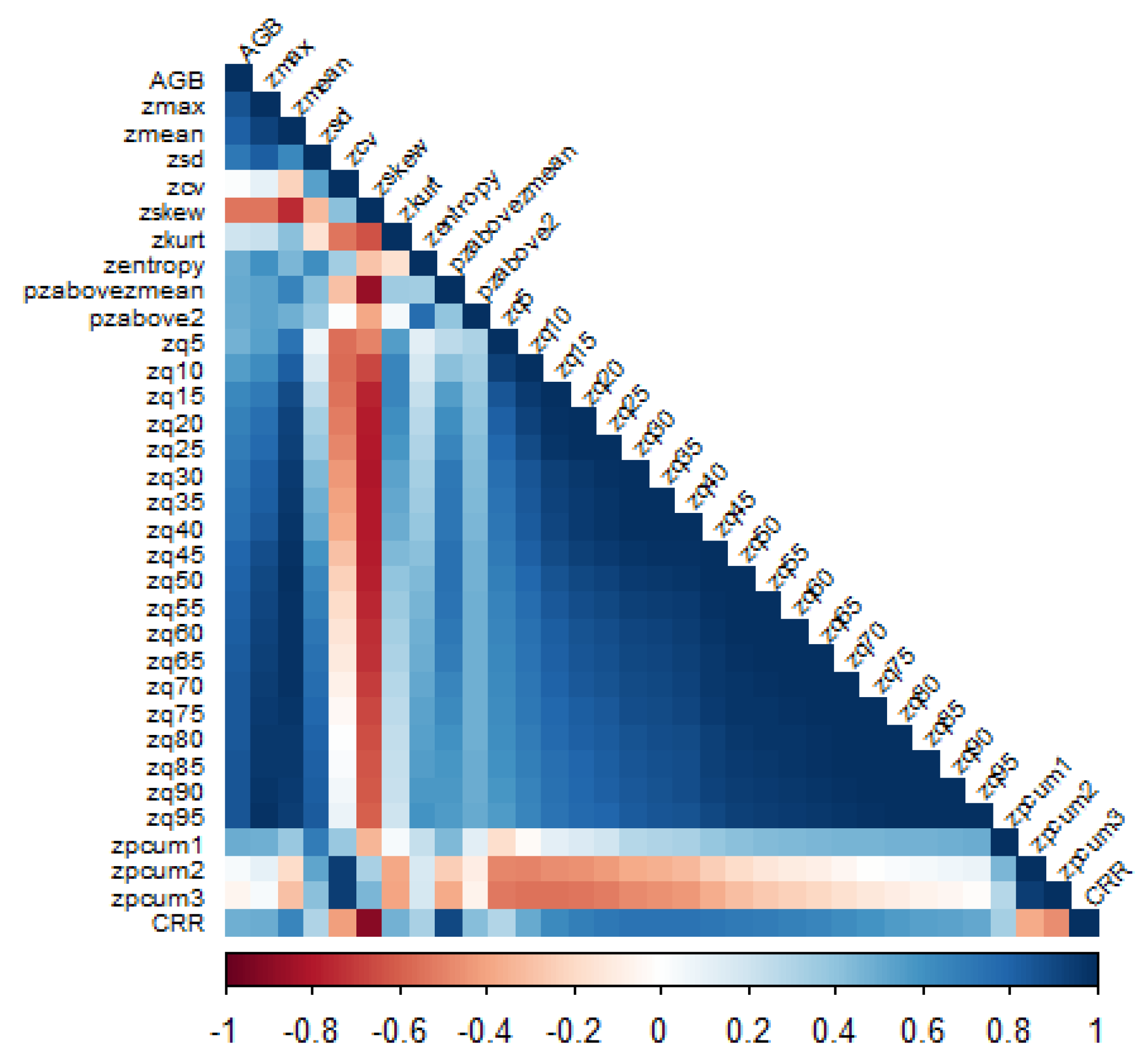
3.2. Correlation between AGB and Predictor Variables

Figure 2 displays the Pearsons’s correlation test (r) between AGB (the dependent variable) and various predictor variables. The result showed that AGB is positively associated with height-related metrics, density-related metrics, and the relative shape of the canopy, and the value ranged from 0.01 to 0.85. However, the higher correlation coefficients (>0.6) between the height metrics and AGB indicated a stronger positive relationship between the percentile height predictor variables and AGB. On the other hand, AGB has a negative relationship with zskew and zcum3, with a correlation coefficient of (≤−0.53), indicating that the increase in height variability would influence the AGB estimation. Predictor variables having moderate (≥0.5 and <0.7) to high (≥7) positive correlations with AGB were selected to fit with the models. The variables with strong positive correlations included zq25 to zq95, zmax, zmean, zsd, and zcv, while the variables with moderate positive correlations included pzabovezmean, pzabove2, zq10 to zq20, zpcum1, CRR, and zentropy, repectively. In summary, the predictor variables that positively correlate with AGB, especially those showing stronger correlations, are better suited as predictor variables for modeling AGB.

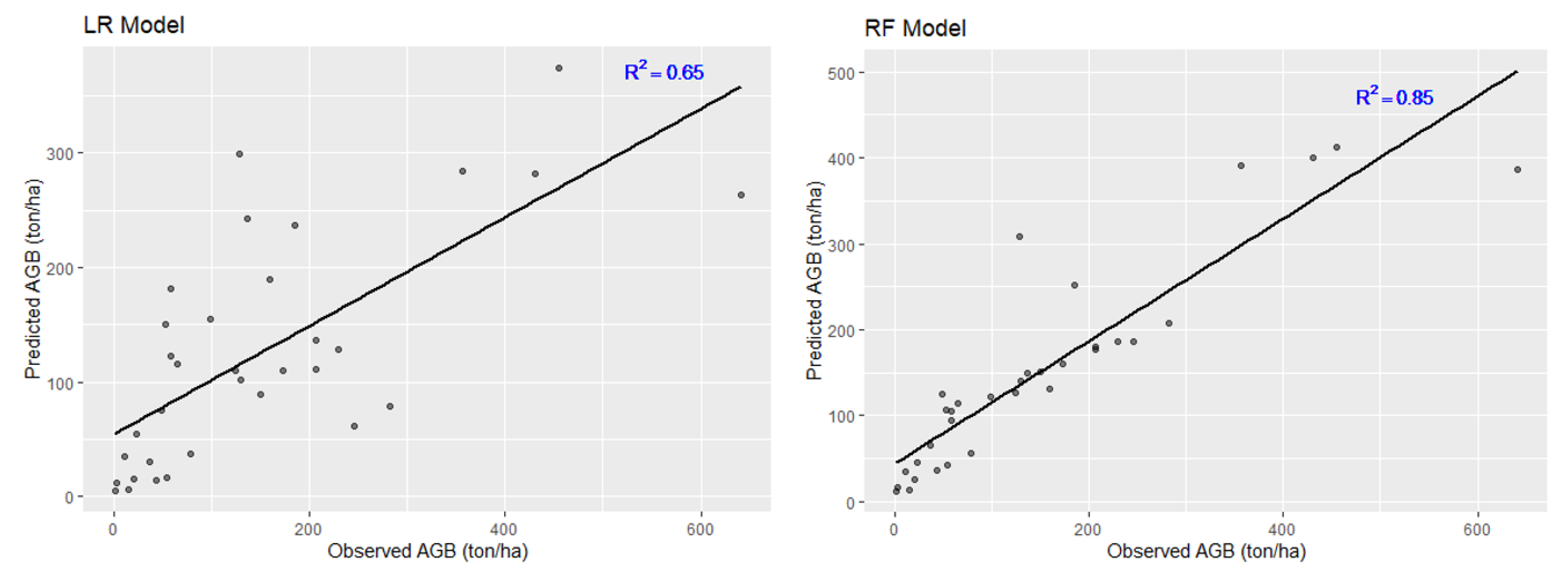
3.3. Linear Regression (LR) Method for Biomass Estimation

The single and multivariable regression models were created to examine the relationship between the log-transformed above-ground biomass (ln(AGB)) as the dependent variable and the LiDAR metrics as the independent variable. Stepwise variable selection determined that the forward selection approach produced the most accurate models, followed by backward selection. The five best models for each response variable are presented in Table 3. Consequently, the model AGB1 was chosen to predict the AGB due to its highest training accuracy (Table 3). As indicated by the calculated VIFs, the assessment of multicollinearity revealed that no variables in any of the models contributed to multicollinearity (VIF < 5).
Furthermore, the p-values indicated that all competitive models were significant; however, the height percentile zq95 was only the significant variable (p < 0.05) in all models (p < 0.05). The values of R2 and RMSE varied across the models, ranging from 0.715 to 0.721 and 85.91 ton/ha to 91.67 ton/ha, respectively. Based on the significant effect of a coefficient and the variability explained by the model, the best model was AGB1, utilizing the height 95th percentile (zq95) variable (R2 = 0.721). Among the LiDAR metrics considered, the height 95th percentile (zq95) was the most effective for estimating AGB.
The model was validated using test data, with an R2 value of 0.65 and RMSE of 105.88 ton/ha (Table 4). The predicted AGB map at 30 × 30 m resolution from the best linear regression model is shown in Figure 3. The values of AGB ranged from 0 to 442 ton/ha, with the mean value of 130 ton/ha.

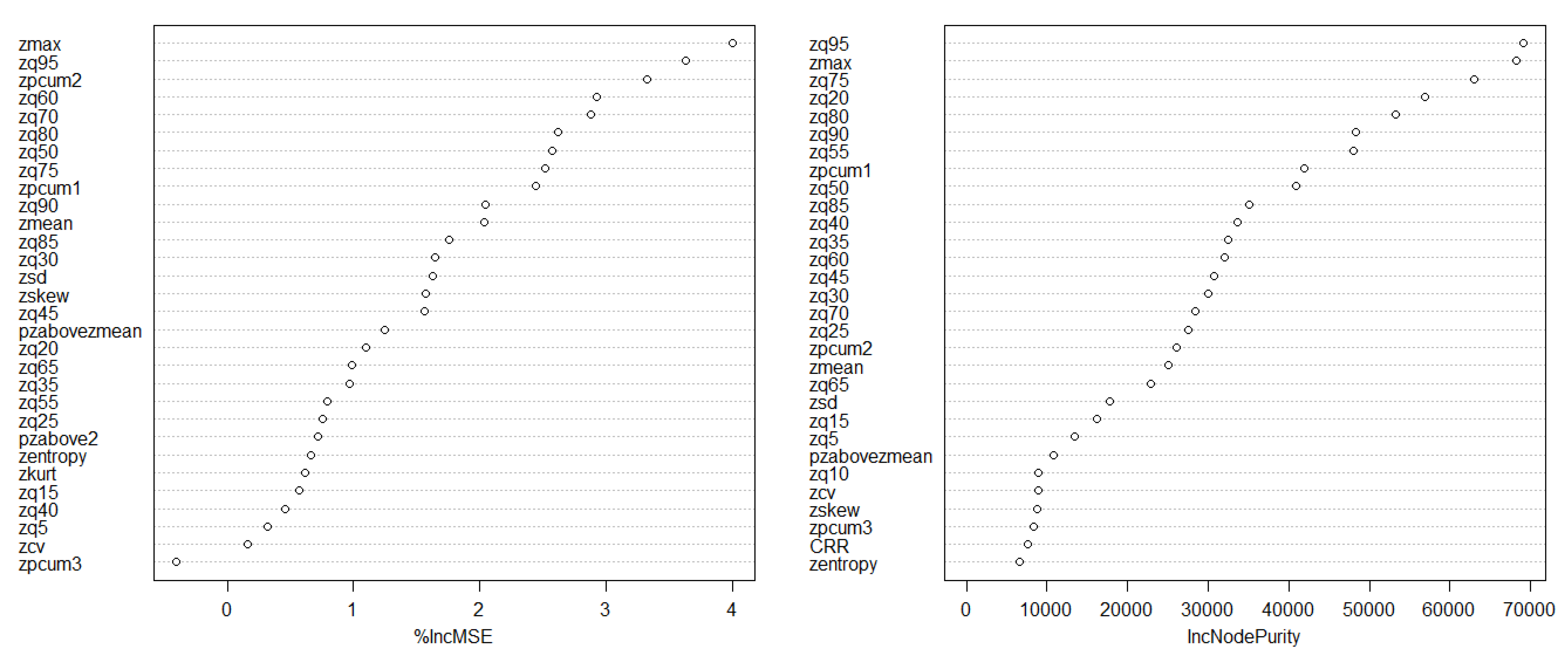
3.4. Random Forest Method for Biomass Estimation

The second approach applied the RF model to estimate the AGB based on LiDAR point metrics. The RF algorithm calculated and plotted the importance of the variables, showing the top variables for predicting AGB are shown in Figure 4.
All the predictor variables were used in the model. However, among them, height-related variables like zmax, zmean, zq75, zq80, zq90, zq95, and density-based variables, zpcum1, and zpcum2, showed relatively higher %IncMSE and IncNodePurity values. The zq95 and zmax are the most essential LiDAR metrics among the top selected variables in the RF model. The following training accuracy was achieved for RF model estimation with an R2 of 0.92 and an RMSE of 41.53 ton/ha. The model was validated with test data and had an accuracy of R2 of 0.85 and RMSE of 60.9 ton/ha (Table 4). The predicted AGB map at 30 × 30 m resolution from the RF model is displayed in Figure 5. The values of AGB ranged from 0 to 446 ton/ha, with the mean value of 120 ton/ha.
The performance of the models was expressed by scatter plots, which showed the relationship between the predicted and observed AGB values for the test data (Figure 6). The RF model showed a higher accuracy than the LR model (Table 4, Figure 6). The R2 increased from 0.65 to 0.85, and the RMSE and MAE values decreased from 105.88 to 60.9 ton/ha and from 75 to 39.7 ton/ha, respectively (Table 4). The random forest AGB model (R2 = 0.85, RMSE = 60.9 ton/ha, and MAE = 39.7 ton/ha), was more effective than the one using a linear regression model (R2 = 0.65, RMSE = 105.88 ton/ha, MAE = 75 ton/ha). As for the RF model, the fitting slope was close to 1, and the scattered points were more evenly distributed around the 1:1 line. The scatter plot features for the RF model revealed more accurate and evenly distributed fit predictions compared to the LR model in ton/ha.

4. Discussion

Selecting suitable remote-sensing variables is critical in AGB estimation [57]. The study used Pearson’s correlation analysis to determine the best predictors. The correlations between the AGB and the predictor variables were mostly positively correlated and positively associated with height percentiles, as shown in Figure 2. Height percentiles are commonly used for AGB estimation since they are highly correlated with AGB [58], yet there is a functional difference between the lower and upper percentiles. The upper percentile is usually used to detect forest growth, and it is better than using maximum height since the latter is less reliable with its low point density [59]. The stepwise variable selection model selected zq95, which was the upper height percentile, which could be due to the canopy that started high above the ground, known as crown base height. Therefore, AGB was more correlated with the upper percentile since it was more representative of the AGB of the study area.
This study used two different modeling methods to estimate the forest AGB: the LR and RF models. Although there were differences in predicting accuracy results between the two methods, their accuracy results indicated that both methods could be used to estimate AGB using ALS data in the study area. The RF model’s accuracy result was better than the LR approach (R2 of 0.85 vs. R2 of 0.65, RMSE of 60.9 ton/ha vs. RMSE of 105.88 ton/ha). These results are consistent with those found by He et al. [60] in a coniferous forest (R2 = 0.73 in the regression model) and by Feng et al. [61] in a mixed forest (R2 = 0.95 with the RF model). Another study conducted by Sung et al. [62] in a tropical forest demonstrated the strong ability of RF to yield better AGB estimation than multiple linear regression. The RF model has been popular and represented to produce a better accuracy than the linear regression model [63].
In the study area, the predicted AGB ranged from 0 to 446 ton/ha with a mean of 120 ton /ha (Figure 5), close to the mean AGB of the field plots. In a study by the Department of Forest Research and Survey (DFRS), Nepal [40], in the forest of the Terai region of Nepal, an estimated average AGB of 190 ton/ha was reported, which is higher than the mean AGB found in the current study using the RF model (120 ton/ha). This difference in estimates might be because the samples represent the entire Terai region and possibly a more mature forest with a more varied species composition than in our study site. Although our study site has a higher number of field sample plots than the DFRS study [40] when considering the area, the representative sample mainly represents the mixed stands of young plantations with natural forest species. In our study area, we found that, within natural stands, Shorea robusta had a higher DBH, height, and AGB than other species, but the stem density was not different. As expected, there was no difference between Eucalpytus and Tectona grandis in stand-level characteristics and AGB. The natural stand had a higher average AGB than the plantation stands, which could be due to the higher stem density and DBH of the associated species. Although incorporating species differences and stand stratification are essential for improving the accuracy of AGB estimates, the optimal AGB estimation models based on the careful selection of data, modeling algorithm, specific forest types, and AGB ranges have been proven to be effective in improving estimation accuracy [55,61,62]. Prediction without stratification could either overestimate at the lower AGB and underestimate at the higher AGB than stratification. However, Zhao et al. [64] did not report any significant difference in the mean AGB estimation between non-stratification and stratification in subtropical forests.
Stand-level AGB estimation often varies with the remote-sensing data acquisition approach [58,65,66]. A study by Singh et al. [65] in the Western Terai Sal Forest of Nepal using an RF model with Sentinel 2 data found that AGB ranged from 118.34 to 425.97 ton/ha. This study provides a reference point for the range of AGB estimates in a similar region. Another study by Rana et al. [40] in a dense tropical forest in Nepal compared AGB estimation techniques. The study showed that ALS prediction techniques had an R2 of 0.73 and RMSE of 62.9 ton/ha, respectively, outperforming RapidEye and Landsat data. Compared to ALS predictors, RapidEye/Landsat predictors have little beneficial effect on increasing accuracy or precision [66,67]. Moreover, the RF non-parametric model was better for estimating AGB than the regression parametric model. Feng et al. [65] observed that LiDAR data provided stable and better AGB estimations than RapidEye in the moist tropical region, and the stratification of vegetation types was not needed for LiDAR data to improve AGB estimation. Likewise, the RF algorithm provides better AGB estimation without classifying forest types, while the LR approach is better with the stratification of forest types [56,62,63,64]. Pandit et al. [68] used two statistical approaches, multiple linear regression (MLR) and RF, to estimate the AGB in the sub-tropical buffer zone community forests of Nepal using Sentinel 2 data. The RF algorithm produced better results (R2 = 0.95 and RMSE = 13.3 ton/ha) than the MLR model (R2 = 0.56 and RMSE = 37.01 ton/ha). The results of the current study are comparable to the findings of the previous studies. However, the choice of prediction methods has a considerable effect on the prediction quality [28,62,63]. The variations in AGB estimates across different studies, can be influenced by factors such as data sources, modeling techniques, and forest characteristics [63,66,67].
Numerous studies have emphasized that the linear regression method’s lower performance is based on the complexity and non-linearity between remote-sensing-based variables and AGB [69,70,71]. Another reason is that the linear regression method is less flexible when facing non-linear problems [28] and cannot adequately handle the multicollinearity problem [72]. One of the advantages of using RF is that it can determine the importance of variables. Variable selection allows the prediction algorithm to focus on relevant variables while ignoring the contribution of irrelevant variables that can be misleading [73]. In the RF model, nine important variables showed a strong relationship with the AGB. Among these variables, the height based metric zq95 and zmax emerged as the most critical features in the RF model, and these were consistent variables found in other studies in predicting AGB [74,75,76]. These variables significantly contributed to reducing errors and enhancing the purity of decision trees within RF models compared to other predictors [77,78]. The other LiDAR metrics, such as density and crown-based predictor variables, were found to be less essential variables in predicting AGB using the RF model. Incorporating the stand attributes such as age with LiDAR-based metrics could better explain the variability in AGB prediction in even-aged managed forests [79]. Although the RF model provides a better selection of features, the LR algorithm cannot effectively delineate the nonlinear and complex relationships between the forest attributes and the AGB [28,34]. When the number of sample plots is insufficient, the LR approach is better than the RF approach, and a sufficient number of samples with relatively low and high AGB must be collected for the RF approach to reduce the over- and under-estimation problems [19,58].
There are some limitations to our study to consider. The LiDAR data used in the study were collected in 2021; thus, the results may not reflect current conditions or changes in forest biomass over time. Moreover, the below-ground forest biomass has been ignored, and further study is required to determine how different forest types influence the AGB distributions. This study did not discuss the potential impact of forest disturbance or management practices on AGB estimation. Although these results are informative, they should be understood within these limitations, and future studies should focus on these limitations in order to gain a more thorough understanding of the matter.
In summary, the RF prediction technique is promising for estimating AGB, as it has often been used in estimating forest parameters. The above-ground biomass maps produced quantify biomass inside the SFDP and can help to estimate ecosystem services such as carbon stock, canopy status, and forest health. This study holds immense potential for facilitating sustainable forest management, climate change mitigation, biodiversity conservation, and land-use planning in the Terai region of Nepal.

5. Conclusions

From the results of this study, it can be concluded that the RF model provided a more significant prediction accuracy than the LR model. This study prepared a 30 m resolution and wall-to-wall forest AGB of the study area by combining field and airborne LiDAR data. The height 95th percentile (zq95) and height maximum (zmax) appeared to be the most significant LiDAR metrics in the RF model for estimating AGB. This study showed that AGB stocks in tropical forests can be predicted with acceptable precision and accuracy using the LiDAR metrics. Therefore, we conclude that airborne LiDAR and field data have significant potential for forest AGB monitoring. This method can be applied to map and monitor forest biomass and carbon stocks in the Terai region of Nepal. The model’s prediction accuracy can be further improved by obtaining dependent variables from extensive sample sizes, combining the use of ALS with multiple remotely sensed data, and using the new methods (e.g., deep learning) in the AGB model.

Author Contributions

Y.B.K. performed research design, data acquisition, data analysis, and manuscript drafting. Q.L. contributed to the conceptualization and supervision. P.S. contributed to the data analysis, review, and editing. D.G. contributed to the visualization and proofreading. H.A. contributed to conceiving research ideas, data analysis, review, and editing. All authors have read and agreed to the published version of the manuscript.

Funding

The China Scholarship Council (CSC 2020SLJ017262) provided funding for this research project.

Data Availability Statement

The data are not publicly available due to the data is designed to be used in other ongoing research and should be protected before official publication.

Acknowledgments

We sincerely thank the Government of Nepal, Ministry of Forests and Environment, Nepal Ban Nigam Limited for generously providing valuable data. Additionally, we would like to thank Arbonaut Ltd., Finland, for their kind support in making these data accessible to us. We thank the Institute of Forestry, Tribhuvan University, Hetauda, Nepal. Furthermore, we are immensely grateful to the Key Laboratory for Silviculture and Conservation of the Ministry of Education, Beijing Forestry University, and the International College of Forestry, Beijing Forestry University, China, for ensuring optimal research conditions for us. Their unwavering commitment to fostering an environment conducive to scientific inquiry has been instrumental in the success of our research endeavor. Hari Adhikari would like to thank Jussi Rasinmäki, Ismo Hippi, and Janne Sarkeala from AFRY OY for their support.

Conflicts of Interest

The authors declare no conflict of interest.

References

  1. Pan, Y.; Birdsey, R.A.; Fang, J.; Houghton, R.; Kauppi, P.E.; Kurz, W.A.; Phillips, O.L.; Shvidenko, A.; Lewis, S.L.; Canadell, J.G.; et al. A large and persistent carbon sink in the world’s forests. Science 2011, 333, 988–993. [Google Scholar] [CrossRef] [PubMed]
  2. Estornell, J.; Ruiz, L.A.; Velázquez-Martí, B.; Fernández-Sarría, A. Estimation of shrub biomass by airborne LiDAR data in small forest stands. For. Ecol. Manag. 2011, 262, 1697–1703. [Google Scholar] [CrossRef]
  3. Frazer, G.W.; Magnussen, S.; Wulder, M.A.; Niemann, K.O. Simulated impact of sample plot size and co-registration error on the accuracy and uncertainty of LiDAR-derived estimates of forest stand biomass. Remote Sens. Environ. 2011, 115, 636–649. [Google Scholar] [CrossRef]
  4. García, M.; Riaño, D.; Chuvieco, E.; Danson, F.M. Estimating biomass carbon stocks for a Mediterranean forest in central Spain using LiDAR height and intensity data. Remote Sens. Environ. 2010, 114, 816–830. [Google Scholar] [CrossRef]
  5. Singh, K.K.; Chen, G.; McCarter, J.B.; Meentemeyer, R.K. Effects of LiDAR point density and landscape context on estimates of urban forest biomass. ISPRS J. Photogramm. Remote Sens. 2015, 101, 310–322. [Google Scholar] [CrossRef]
  6. Cusack, D.F.; Axsen, J.; Shwom, R.; Hartzell-Nichols, L.; White, S.; Mackey, K.R.M. An interdisciplinary assessment of climate engineering strategies. Front. Ecol. Environ. 2014, 12, 280–287. [Google Scholar] [CrossRef] [PubMed]
  7. Kauranne, T.; Joshi, A.; Gautam, B.; Manandhar, U.; Nepal, S.; Peuhkurinen, J.; Hämäläinen, J.; Junttila, V.; Gunia, K.; Latva-Käyrä, P.; et al. LiDAR-Assisted Multi-Source Program (LAMP) for measuring above ground biomass and forest carbon. Remote Sens. 2017, 9, 154. [Google Scholar] [CrossRef]
  8. Urbazaev, M.; Thiel, C.; Cremer, F.; Dubayah, R.; Migliavacca, M.; Reichstein, M.; Schmullius, C. Estimation of forest aboveground biomass and uncertainties by integration of field measurements, airborne LiDAR, and SAR and optical satellite data in Mexico. Carbon Balance Manag. 2018, 13, 5. [Google Scholar] [CrossRef]
  9. Hussin, Y.A.; Gilani, H.; Van Leeuwen, L.; Murthy, M.S.R.; Shah, R.; Baral, S.; Tsendbazar, N.E.; Shrestha, S.; Shah, S.K.; Qamer, F.M. Evaluation of object-based image analysis techniques on very high-resolution satellite image for biomass estimation in a watershed of hilly forest of Nepal. Appl. Geomat. 2014, 6, 59–68. [Google Scholar] [CrossRef]
  10. IPCC. AR4 Climate Change 2007: Impacts, Adaptation, and Vulnerability; IPCC: New York, NY, USA, 2007. [Google Scholar]
  11. Duncanson, L.; Disney, M.; Armston, J.; Nickeson, J.; Minor, D. Committee on Earth Observation Satellites Working Group on Calibration and Validation Land Product Validation Subgroup Aboveground Woody Biomass Product Validation Good Practices Protocol. In Good Practices for Satellite Derived Land Product Validation; Land Product Validation Subgroup (WGCV/CEOS): Washington, DC, USA, 2021; p. 236. [Google Scholar] [CrossRef]
  12. Houghton, R.A.; Hall, F.; Goetz, S.J. Importance of biomass in the global carbon cycle. J. Geophys. Res. Biogeosci. 2009, 114, 1–13. [Google Scholar] [CrossRef]
  13. Qureshi, A.; Pariva; Badola, R.; Hussain, S.A. A review of protocols used for assessment of carbon stock in forested landscapes. Environ. Sci. Policy 2012, 16, 81–89. [Google Scholar] [CrossRef]
  14. Stovall, A.E.L.; Vorster, A.G.; Anderson, R.S.; Evangelista, P.H.; Shugart, H.H. Non-destructive aboveground biomass estimation of coniferous trees using terrestrial LiDAR. Remote Sens. Environ. 2017, 200, 31–42. [Google Scholar] [CrossRef]
  15. Brown, S.; Lugo, A.E. Aboveground biomass estimates for tropical moist forests of the Brazilian Amazon. Interciencia. Caracas 1992, 17, 8–18. [Google Scholar]
  16. Chave, J.; Andalo, C.; Brown, S.; Cairns, M.A.; Chambers, J.Q.; Eamus, D.; Fölster, H.; Fromard, F.; Higuchi, N.; Kira, T.; et al. Tree allometry and improved estimation of carbon stocks and balance in tropical forests. Oecologia 2005, 145, 87–99. [Google Scholar] [CrossRef] [PubMed]
  17. Du, L.; Zhou, T.; Zou, Z.; Zhao, X.; Huang, K.; Wu, H. Mapping forest biomass using remote sensing and national forest inventory in China. Forests 2014, 5, 1267–1283. [Google Scholar] [CrossRef]
  18. Tang, X.; Kleinn, C.; Guan, F.; Forrester, D.I.; Guisasola, R. Inventory-based estimation of forest biomass in Shitai County, China: A comparison of five methods. Ann. For. Res. 2016, 59, 269–280. [Google Scholar] [CrossRef]
  19. Dang, A.T.N.; Nandy, S.; Srinet, R.; Luong, N.V.; Ghosh, S.; Senthil Kumar, A. Forest aboveground biomass estimation using machine learning regression algorithm in Yok Don National Park, Vietnam. Ecol. Inform. 2019, 50, 24–32. [Google Scholar] [CrossRef]
  20. Mura, M.; McRoberts, R.E.; Chirici, G.; Marchetti, M. Estimating and mapping forest structural diversity using airborne laser scanning data. Remote Sens. Environ. 2015, 170, 133–142. [Google Scholar] [CrossRef]
  21. Sačkov, I.; Santopuoli, G.; Bucha, T.; Lasserre, B.; Marchetti, M. Forest inventory attribute prediction using lightweight aerial scanner data in a selected type of multilayered deciduous forest. Forests 2016, 7, 307. [Google Scholar] [CrossRef]
  22. Hyyppä, J.; Hyyppä, H.; Xiaowei, Y.; Kaartinen, H.; Kukko, A.; Holopainen, M. Topographic Laser Ranging and Scanning: Principles and Processing; CRC Press Taylor & Francis Group: Boca Raton, FL, USA, 2009; pp. 335–370. [Google Scholar]
  23. Zhao, K.; Popescu, S. Lidar-based mapping of leaf area index and its use for validating GLOBCARBON satellite LAI product in a temperate forest of the southern USA. Remote Sens. Environ. 2009, 113, 1628–1645. [Google Scholar] [CrossRef]
  24. Hawryło, P.; Tompalski, P.; Wȩzyk, P. Area-based estimation of growing stock volume in Scots pine stands using ALS and airborne image-based point clouds. Forestry 2017, 90, 686–696. [Google Scholar] [CrossRef]
  25. Maxwell, A.E.; Warner, T.A.; Fang, F. Implementation of machine-learning classification in remote sensing: An applied review. Int. J. Remote Sens. 2018, 39, 2784–2817. [Google Scholar] [CrossRef]
  26. Chen, L.; Ren, C.; Zhang, B.; Wang, Z.; Xi, Y. Estimation of forest above-ground biomass by geographically weighted regression and machine learning with sentinel imagery. Forests 2018, 9, 582. [Google Scholar] [CrossRef]
  27. Hudak, A.T.; Crookston, N.L.; Evans, J.S.; Hall, D.E.; Falkowski, M.J. Nearest neighbor imputation of species-level, plot-scale forest structure attributes from LiDAR data. Remote Sens. Environ. 2008, 112, 2232–2245. [Google Scholar] [CrossRef]
  28. Liu, K.; Wang, J.; Zeng, W.; Song, J. Comparison and evaluation of three methods for estimating forest above ground biomass using TM and GLAS data. Remote Sens. 2017, 9, 341. [Google Scholar] [CrossRef]
  29. Gobakken, T.; Næsset, E.; Nelson, R.; Bollandsås, O.M.; Gregoire, T.G.; Ståhl, G.; Holm, S.; Ørka, H.O.; Astrup, R. Estimating biomass in Hedmark County, Norway using national forest inventory field plots and airborne laser scanning. Remote Sens. Environ. 2012, 123, 443–456. [Google Scholar] [CrossRef]
  30. Kankare, V.; Räty, M.; Yu, X.; Holopainen, M.; Vastaranta, M.; Kantola, T.; Hyyppä, J.; Hyyppä, H.; Alho, P.; Viitala, R. Single tree biomass modelling using airborne laser scanning. ISPRS J. Photogramm. Remote Sens. 2013, 85, 66–73. [Google Scholar] [CrossRef]
  31. Luo, S.; Wang, C.; Xi, X.; Pan, F.; Peng, D.; Zou, J.; Nie, S.; Qin, H. Fusion of airborne LiDAR data and hyperspectral imagery for aboveground and belowground forest biomass estimation. Ecol. Indic. 2017, 73, 378–387. [Google Scholar] [CrossRef]
  32. Rana, P.; Korhonen, L.; Gautam, B.; Tokola, T. Effect of field plot location on estimating tropical forest above-ground biomass in Nepal using airborne laser scanning data. ISPRS J. Photogramm. Remote Sens. 2014, 94, 55–62. [Google Scholar] [CrossRef]
  33. Wu, B.; Yu, B.; Yue, W.; Shu, S.; Tan, W.; Hu, C.; Huang, Y.; Wu, J.; Liu, H. A voxel-based method for automated identification and morphological parameters estimation of individual street trees from mobile laser scanning data. Remote Sens. 2013, 5, 584–611. [Google Scholar] [CrossRef]
  34. White, J.C.; Coops, N.C.; Wulder, M.A.; Vastaranta, M.; Hilker, T.; Tompalski, P. Remote Sensing Technologies for Enhancing Forest Inventories: A Review. Can. J. Remote Sens. 2016, 42, 619–641. [Google Scholar] [CrossRef]
  35. Zolkos, S.G.; Goetz, S.J.; Dubayah, R. A meta-analysis of terrestrial aboveground biomass estimation using lidar remote sensing. Remote Sens. Environ. 2013, 128, 289–298. [Google Scholar] [CrossRef]
  36. Li, M.; Im, J.; Quackenbush, L.J.; Liu, T. Forest biomass and carbon stock quantification using airborne LiDAR data: A case study over huntington wildlife forest in the Adirondack park. IEEE J. Sel. Top. Appl. Earth Obs. Remote Sens. 2014, 7, 3143–3156. [Google Scholar] [CrossRef]
  37. Lefsky, M.A.; Harding, D.J.; Keller, M.; Cohen, W.B.; Carabajal, C.C.; Del Bom Espirito-Santo, F.; Hunter, M.O.; de Oliveira, R. Estimates of forest canopy height and aboveground biomass using ICESat. Geophys. Res. Lett. 2005, 32, 1–4. [Google Scholar] [CrossRef]
  38. Gopalakrishnan, R.; Thomas, V.A.; Coulston, J.W.; Wynne, R.H. Prediction of canopy heights over a large region using heterogeneous lidar datasets: Efficacy and challenges. Remote Sens. 2015, 7, 11036–11060. [Google Scholar] [CrossRef]
  39. de Almeida, C.T.; Galvão, L.S.; de Oliveira Cruz e Aragão, L.E.; Ometto, J.P.H.B.; Jacon, A.D.; de Souza Pereira, F.R.; Sato, L.Y.; Lopes, A.P.; de Alencastro Graça, P.M.L.; de Jesus Silva, C.V.; et al. Combining LiDAR and hyperspectral data for aboveground biomass modeling in the Brazilian Amazon using different regression algorithms. Remote Sens. Environ. 2019, 232, 111323. [Google Scholar] [CrossRef]
  40. DFRS. STATE of NEPAL’s FORESTS; Department of Forest Research and Survey: Kathmandu, Nepal, 2015; ISBN 9789937889636.
  41. Kandel, P.N. Estimation of above Ground Forest Biomass and Carbon Stock by Integrating Lidar, Satellite Image and Field Measurement in Nepal. J. Nat. Hist. Mus. 2015, 28, 160–170. [Google Scholar] [CrossRef]
  42. Karna, Y.K.; Hussin, Y.A.; Gilani, H.; Bronsveld, M.C.; Murthy, M.S.R.; Qamer, F.M.; Karky, B.S.; Bhattarai, T.; Aigong, X.; Baniya, C.B. Integration of WorldView-2 and airborne LiDAR data for tree species level carbon stock mapping in Kayar Khola watershed, Nepal. Int. J. Appl. Earth Obs. Geoinf. 2015, 38, 280–291. [Google Scholar] [CrossRef]
  43. Murthy, M.S.R.; Wesselman, S.; Gilani, H. Multi-Scale Forest Biomass Assessment and Monitoring in the Hindu Kush Himalayan Region: A Geospatial Perspective; International Centre for Integrated Mountain Development (ICIMOD): Kathmandu, Nepal, 2015. [Google Scholar]
  44. Rana, P.; Popescu, S.; Tolvanen, A.; Gautam, B.; Srinivasan, S.; Tokola, T. Estimation of tropical forest aboveground biomass in Nepal using multiple remotely sensed data and deep learning. Int. J. Remote Sens. 2023, 44, 5147–5171. [Google Scholar] [CrossRef]
  45. FRA/DFRS. Forest Resource Assessment Nepal Project/Department of Forest Research and Survey; FRA/DFRS: Kathmandu, Nepal, 2014. [Google Scholar]
  46. Sharma, E.R.; Pukkala, T. Volume Equations and Biomass Prediction of Forest Trees in Nepal; MoFSC: Kathmandu, Nepal, 1990; Available online: https://www.worldcat.org/title/volume-equations-and-biomass-prediction-of-forest-trees-in-nepal/oclc/49714635 (accessed on 5 February 2024).
  47. MoFSC. Master Plan for the Forestry Sector in Nepal; MoFSC: Kathmandu, Nepal, 1988. [Google Scholar]
  48. Roussel, J.R.; Auty, D.; Coops, N.C.; Tompalski, P.; Goodbody, T.R.H.; Meador, A.S.; Bourdon, J.F.; de Boissieu, F.; Achim, A. lidR: An R package for analysis of Airborne Laser Scanning (ALS) data. Remote Sens. Environ. 2020, 251, 112061. [Google Scholar] [CrossRef]
  49. Breusch, A.R.; Pagan, T.S. A Simple Test for Heteroscedasticity and Random Coefficient Variation. Econometrica 1979, 47, 1287–1294. [Google Scholar] [CrossRef]
  50. Sheridan, R.D.; Popescu, S.C.; Gatziolis, D.; Morgan, C.L.S.; Ku, N.W. Modeling Forest Aboveground Biomass and Volume Using Airborne LiDAR Metrics and Forest Inventory and Analysis Data in the Pacific Northwest. Remote Sens. 2015, 7, 229–255. [Google Scholar] [CrossRef]
  51. Belgiu, M.; Csillik, O. Sentinel-2 cropland mapping using pixel-based and object-based time-weighted dynamic time warping analysis. Remote Sens. Environ. 2018, 204, 509–523. [Google Scholar] [CrossRef]
  52. Freeman, E.A.; Frescino, T.S.; Moisen, G.G. ModelMap: An R Package for Model Creation and Map Production. 2023. Available online: https://cran.r-project.org/web/packages/ModelMap/vignettes/VModelMap.pdf (accessed on 5 February 2024).
  53. Kuhn, M. Building Predictive Models in R Using the caret Package. J. Stat. Softw. 2008, 28. [Google Scholar] [CrossRef]
  54. R Core Team. A Language and Environment for Statistical Computing; R Foundation for Statistical Computing: Vienna, Austria, 2020; Available online: www.R-project.org (accessed on 5 February 2024).
  55. Vafaei, S.; Soosani, J.; Adeli, K.; Fadaei, H.; Naghavi, H.; Pham, T.D.; Bui, D.T. Improving accuracy estimation of Forest Aboveground Biomass based on incorporation of ALOS-2 PALSAR-2 and Sentinel-2A imagery and machine learning: A case study of the Hyrcanian forest area (Iran). Remote Sens. 2018, 10, 172. [Google Scholar] [CrossRef]
  56. Jiang, X.; Li, G.; Lu, D.; Chen, E.; Wei, X. Stratification-Based Forest Aboveground Biomass Estimation in a Subtropical Region Using Airborne Lidar Data. Remote Sens. 2020, 12, 1101. [Google Scholar] [CrossRef]
  57. Lu, D. The Potential and Challenge of Remote Sensing—Based Biomass Estimation. Int. J. Remote Sens. 2006, 27, 1297–1328. [Google Scholar] [CrossRef]
  58. Lim, K.S.; Treitz, P.M. Estimation of above ground forest biomass from airborne discrete return laser scanner data using canopy-based quantile estimators. Scand. J. For. Res. 2004, 19, 558–570. [Google Scholar] [CrossRef]
  59. Cao, L.; Coops, N.C.; Innes, J.L.; Sheppard, S.R.J.; Fu, L.; Ruan, H.; She, G. Estimation of forest biomass dynamics in subtropical forests using multi-temporal airborne LiDAR data. Remote Sens. Environ. 2016, 178, 158–171. [Google Scholar] [CrossRef]
  60. He, Q.; Chen, E.; An, R.; Li, Y. Above-ground biomass and biomass components estimation using LiDAR data in a coniferous forest. Forests 2013, 4, 984–1002. [Google Scholar] [CrossRef]
  61. Feng, Y.; Lu, D.; Chen, Q.; Keller, M.; Moran, E.; dos-Santos, M.N.; Bolfe, E.L.; Batistella, M. Examining effective use of data sources and modeling algorithms for improving biomass estimation in a moist tropical forest of the Brazilian Amazon. Int. J. Digit. Earth 2017, 10, 996–1016. [Google Scholar] [CrossRef]
  62. Sun, X.; Li, G.; Wang, M.; Fan, Z. Analyzing the uncertainty of estimating forest aboveground biomass using optical imagery and spaceborne LiDAR. Remote Sens. 2019, 11, 722. [Google Scholar] [CrossRef]
  63. Gao, Y.; Lu, D.; Li, G.; Wang, G.; Chen, Q.; Liu, L.; Li, D. Comparative analysis of modeling algorithms for forest aboveground biomass estimation in a subtropical region. Remote Sens. 2018, 10, 627. [Google Scholar] [CrossRef]
  64. Zhao, P.; Lu, D.; Wang, G.; Wu, C.; Huang, Y.; Yu, S. Examining spectral reflectance saturation in landsat imagery and corresponding solutions to improve forest aboveground biomass estimation. Remote Sens. 2016, 8, 469. [Google Scholar] [CrossRef]
  65. Singh, B.; Verma, A.K.; Tiwari, K.; Joshi, R. Above ground tree biomass modeling using machine learning algorithms in western Terai Sal Forest of Nepal. Heliyon 2023, 9, e21485. [Google Scholar] [CrossRef] [PubMed]
  66. Cao, L.; Pan, J.; Li, R.; Li, J.; Li, Z. Integrating airborne LiDAR and optical data to estimate forest aboveground biomass in arid and semi-arid regions of China. Remote Sens. 2018, 10, 532. [Google Scholar] [CrossRef]
  67. Hou, Z.; Xu, Q.; Tokola, T. Use of ALS, Airborne CIR and ALOS AVNIR-2 data for estimating tropical forest attributes in Lao PDR. ISPRS J. Photogramm. Remote Sens. 2011, 66, 776–786. [Google Scholar] [CrossRef]
  68. Pandit, S.; Tsuyuki, S.; Dube, T. Estimating above-ground biomass in sub-tropical buffer zone community forests, Nepal, using Sentinel 2 data. Remote Sens. 2018, 10, 601. [Google Scholar] [CrossRef]
  69. Baccini, A.; Friedl, M.A.; Woodcock, C.E.; Warbington, R. Forest biomass estimation over regional scales using multisource data. Geophys. Res. Lett. 2004, 31. [Google Scholar] [CrossRef]
  70. Foody, G.M.; Boyd, D.S.; Cutler, M.E.J. Predictive relations of tropical forest biomass from Landsat TM data and their transferability between regions. Remote Sens. Environ. 2003, 85, 463–474. [Google Scholar] [CrossRef]
  71. Muukkonen, P.; Heiskanen, J. Estimating biomass for boreal forests using ASTER satellite data combined with standwise forest inventory data. Remote Sens. Environ. 2005, 99, 434–447. [Google Scholar] [CrossRef]
  72. Ju, C.; Cai, T.; Yang, X. Topography-based modeling to estimate percent vegetation cover in semi-arid Mu Us sandy land, China. Comput. Electron. Agric. 2008, 64, 133–139. [Google Scholar] [CrossRef]
  73. Li, Y.; Li, C.; Li, M.; Liu, Z. Influence of variable selection and forest type on forest aboveground biomass estimation using machine learning algorithms. Forests 2019, 10, 1073. [Google Scholar] [CrossRef]
  74. Woodcock, C.; Song, C. Mapping Forest Aboveground Biomass Using Multisource Remotely Sensed Data. Remote Sens. 2022, 14, 1115. [Google Scholar]
  75. Hong, Y.; Xu, J.; Wu, C.; Pang, Y.; Zhang, S.; Chen, D.; Yang, B. Combining Multisource Data and Machine Learning Approaches for Multiscale Estimation of Forest Biomass. Forests 2023, 14, 2248. [Google Scholar] [CrossRef]
  76. Zhang, L.; Zhang, X.; Shao, Z.; Jiang, W.; Gao, H. Integrating Sentinel-1 and 2 with LiDAR data to estimate aboveground biomass of subtropical forests in northeast Guangdong, China. Int. J. Digit. Earth 2023, 16, 158–182. [Google Scholar] [CrossRef]
  77. Varo-martinez, M.A.; Rachid-casnati, C. Stand Characterization of Eucalyptus spp. Plantations in Uruguay Using Airborne Lidar Scanner Technology. Remote Sens. 2020, 12, 3947. [Google Scholar]
  78. Yan, M.; Xia, Y.; Yang, X.; Wu, X.; Yang, M.; Wang, C.; Hou, Y.; Wang, D. Biomass Estimation of Subtropical Arboreal Forest at Single Tree Scale Based on Feature Fusion of Airborne LiDAR Data and Aerial Images. Sustainability 2023, 15, 1676. [Google Scholar] [CrossRef]
  79. Soriano-Luna, M.; de Los, Á.; Ángeles-Pérez, G.; Guevara, M.; Birdsey, R.; Pan, Y.; Vaquera-Huerta, H.; Valdez-Lazalde, J.R.; Johnson, K.D.; Vargas, R. Determinants of above-ground biomass and its spatial variability in a temperate forest managed for timber production. Forests 2018, 9, 490. [Google Scholar] [CrossRef]
Figure 1. Study area location and forest sample plots. (a) Nepal, (b) the study area.
Land 13 00213 g001
Figure 2. Pearson’s correlation coefficients between AGB and LiDAR metric variables. The number represents the strength, while the color of a square represents the direction (+/−) of the correlation between variables. Negative (red) numbers indicate that the corresponding variables are negatively correlated and are colored in red, whereas positive (blue) numbers represent positive correlations.
Land 13 00213 g002
Figure 3. Forest above-ground biomass map from the linear regression model: (a) western cluster and (b) eastern cluster of the study area.
Land 13 00213 g003
Figure 4. Importance of variables, percentage of the increase in mean squared error (%lncMSE, left panel), and the increase in node purity (IncNodePurity, right panel) for AGB estimation in the random forest model.
Land 13 00213 g004
Figure 5. Forest above-ground biomass map from the random forest model: (a) western cluster and (b) eastern cluster of the study area.
Land 13 00213 g005
Figure 6. The scatter plot shows the field-observed forest AGB (ton/ha) versus predicted forest AGB (ton/ha) using the test data in the RF and LR models.
Land 13 00213 g006
Table 1. Predictors variables used in modeling.
LiDAR MetricsMetricsDescription
Height-related metricsPercentile height zq5, zq10, zq15, zq20, zq25, zq30, zq35, zq40, zq45, zq50, zq55, zq60, zq65, zq70, zq75, zq80, zq85, zq90, zq95The percentiles of the height distributions (5th, 10th, 15th, 20th, 25th, 30th, 35th, 40th, 45th, 50th, 55th, 60th, 65th, 70th, 75th, 80th, 85th, 90th, 95th) of all points above 2 m
Maximum height (zmax)The maximum height above 2 m of all points
Mean height (zmean)The mean height above 2 m of all points
The coefficient of variation in height (zcv)The coefficient of variation in heights of all points above 2 m
Standard deviation (zsd)The standard deviation of heights of all points above 2 m
zskewThe skewness of heights of all points above 2 m
zkurtThe kurtosis of the heights of all points above 2 m
zentropyThe entropy of height distribution
Density-related metricspzabove2Percentages of first returns above 2 m
pzabovezmeanPercentage of returns > mean returns height
zpcum1Cumulative percentage of first returns in the lower 10% of maximum elevation
zpcum2Cumulative percentage of first returns in the lower 20% of maximum elevation
zpcum3Cumulative percentage of first returns in the lower 30% of maximum elevation
The relative shape of the canopyCRRCanopy relief ratio = (Height.mean − Height.min)/(Height.max − Height.min)
Table 2. Descriptive statistics of plot-level inventory plots.
AttributesMeanMinimumMaximumStandard Deviation
Density (trees/ha)462392122343
DBH (cm)24610114
Height (m)172287
Basal area (m2)120.24710
Volume (m3/ha)1080.6519112
AGB (ton/ha)1311640137
Table 3. Different linear regression models and training accuracy.
ModelEquationR2RMSE (ton/ha)
AGB1ln(AGB) = 0.321 + 0.205 × zq950.72191.67
AGB2ln(AGB) = 0.3211 + 0.205 × zq95 + 0.002 × zsd0.71691.59
AGB3ln(AGB) = −0.073 + 0.197 × zq95 + 0.008 × zsd + 0.009 × pzabovezmean0.71290.63
AGB4ln(AGB) = 0.520 +0.215 × Zq95 − 0.129 × zsd + 0.000 × pzabovezmean +0.186 × zpcum10.71786.15
AGB5ln(AGB) = 0.623 + 0.207 × zq95 − 0.091 × zsd − 0.029 × pzabovezmean + 0.183 × zpcum1 + 2.609 × CRR0.71585.91
Table 4. Training and testing accuracy of the RF and LR models.
ModelTraining Data Test Data
R2RMSEMAER2RMSE (ton/ha)MAE
(ton/ha)
Linear regression0.7291.7563.20.65105.8875
Random forest0.9241.5325.270.8560.939.7
Disclaimer/Publisher’s Note: The statements, opinions and data contained in all publications are solely those of the individual author(s) and contributor(s) and not of MDPI and/or the editor(s). MDPI and/or the editor(s) disclaim responsibility for any injury to people or property resulting from any ideas, methods, instructions or products referred to in the content.

