Article

An Enhanced Algorithm for Active Fire Detection in Croplands Using Landsat-8 OLI Data

1
School of Earth Science and Resources, Chang’an University, 126 Yanta Road, Xi’an 710054, China
2
School of Geological Engineering and Geomatics, Chang’an University, 126 Yanta Road, Xi’an 710054, China
*
Author to whom correspondence should be addressed.
Land 2023, 12(6), 1246; https://doi.org/10.3390/land12061246
Submission received: 9 May 2023 / Revised: 11 June 2023 / Accepted: 15 June 2023 / Published: 18 June 2023
(This article belongs to the Section Land – Observation and Monitoring)

Abstract

:
Burning biomass exacerbates or directly causes severe air pollution. The traditional active fire detection (AFD) methods are limited by the thresholds of the algorithms and the spatial resolution of remote sensing images, which misclassify some small-scale fires. AFD for burning straw is interfered with by highly reflective buildings around urban and rural areas, resulting in high commission error (CE). To solve these problems, we developed a multicriteria threshold AFD for burning straw (SAFD) based on Landsat-8 imagery in the context of croplands. In solving the problem of the high CE of highly reflective buildings around urban and rural areas, the SAFD algorithm, which was based on the LightGBM machine learning method (SAFD-LightGBM), was proposed to differentiate active fires from highly reflective buildings with a sample dataset of buildings and active fires and an optimal feature combining spectral features and texture features using the ReliefF feature selection method. The results revealed that the SAFD-LightGBM method performed better than the traditional threshold method, with CE and omission error (OE) of 13.2% and 11.5%, respectively. The proposed method could effectively reduce the interference of highly reflective buildings for active fire detection, and it has general applicability and stability for detecting discrete, small-scale fires in urban and rural areas.

1. Introduction

Biomass burning because of human activities has become one of the main sources of emissions in air pollution management [1,2]. China has the largest agricultural enterprise worldwide with an estimated 1.4 million km2 of area for crop production [3,4]. Agricultural burning in China was estimated to contribute ~3–6% to global agricultural fires [5]. The agricultural burning component is mainly straw, which creates fires different from forest fires. The average forest fire burns more than 104 m2 and sometimes more than 106 m2. Since the average cultivated area of a farming household is very limited in China (around 104 m2), each agricultural fire burns within a small extent [6]. Straw burning usually occurs during the harvest season, with specific regularity that is more frequent than forest fires. Crop straw burning constitutes a major portion of biomass burning by releasing a large amount of particulate matter (PM) and gaseous pollutants into the atmosphere [7]. Therefore, it is of great significance to study the burning of straw around rural areas in China.
Most traditional field methods for monitoring burning biomass use a bottom-up ground survey approach, which requires extensive human and material resources and can only be achieved through point monitoring. There is significant uncertainty in estimating the spatial distribution of burning biomass at the macroscopic scale, and it is difficult to obtain accurate spatiotemporal information about active fires [8]. Remote sensing technology has become an effective method, with its fast, simple, and macroscopic advantages for monitoring burning fires. Applying remote sensing technology to small-scale AFD can provide strong support for environmental improvement and management [9] and is of critical importance for practical research.
Satellite sensors have been widely used for monitoring the spatiotemporal distribution of regional and global active fires [10,11,12]. Most of the existing AFD algorithms are based on sensors with moderate or low spatial resolutions [13,14,15,16]. Moreover, the existing global monitoring systems for active fires mainly utilize polar-orbiting satellites (1 km) or geostationary satellite data with mid-infrared (3–4 μm) and thermal infrared (10–12 μm) bands [14,17,18]. These satellites can be used for near real-time monitoring of large-scale active fires with rapid response capabilities [19]. However, their spatial resolution may not meet the requirements for detecting small-scale fires, resulting in many small-scale fires being missed [2]. Detecting small-scale fires remains challenging and requires more time-consistent satellite data with higher resolution than simple observations of burned areas.
With the development of moderate and high-resolution satellite sensors with SWIR bands, for instance, Landsat-8 and Sentinel-2 (2A, 2B), multispectral images are available for active fire detection. The Landsat-8 OLI sensor has a 16-day revisit period with 30-m spatial resolution, and 15 m resolution can be obtained after image fusion [20]. The Sentinel-2 MSI sensor is also available, with revisit periods of 5 days or less and resolutions of 10 m, 20 m, and 60 m in the visible (VIS) to short-wave infrared (SWIR) bands [21]. It has been established that a suitable spatiotemporal resolution for AFD can be achieved by integrating the available sensors with moderate and high spatial resolution [22,23,24].
Previous studies have established a variety of AFD algorithms based on the reflectance difference of Landsat-8 data, including threshold methods (single threshold, multithreshold, dynamic threshold) and contextual algorithms [10,19,25,26,27,28]. Schroeder et al. [28] developed daytime and nighttime AFD algorithms based on the proposed threshold algorithms using ASTER and Landsat-7 ETM data, and they improved the CE using a multitemporal analytical method [25,27]. Murphy et al. [19] proposed an improved Landsat-8 Temporal Contextual Analysis (CA) algorithm based on the algorithms established by Giglio et al. [25] and Schroeder et al. [27,28]. Kumar and Roy [26] proposed a Landsat-8 AFD algorithm (GOLI) using fixed reflectance thresholds, and its results had lower CE compared with the algorithms proposed by Murphy et al. [19] and Schroeder et al. [28]. A U-Net deep learning AFD algorithm of Landsat-8 data revealed better accuracy than the traditional threshold model [29]. These AFD algorithms use images with higher spatial resolution, and they are capable of detecting smaller-scale fires, reducing the CE and improving the accuracy compared with traditional methods.
However, Landsat-8′s reflectance-based threshold and deep learning AFD algorithms may still be interfered with by potential false detections. Interference from highly reflective buildings is a considerable problem for AFD in urban and rural areas [26,28,30,31]. These persistent effects of highly reflective buildings have generally been solved by multitemporal analytical methods or by fixing thresholds [19,28]. The multitemporal analytical method proposed by Schroeder et al. [28] was applied to urban areas, and they found that the CE reached 34.6%. The CA (Contextual Analysis) algorithm was used for AFD in urban areas using single-view Landsat-8 imagery, generating an average of more than 500 false pixels and up to 3400 false pixels [19]. Some algorithms avoid potential misclassification by not selecting urban areas as the study area [26]. Researchers have tried to improve the problem of highly reflective buildings being misclassified as active fires, but it has still not been well resolved [22,30].
Machine learning methods have been widely used for classification via remote sensing because of its advantages of encoding more complex rules with more accurate weights, coefficients, and threshold settings [32]. Using a weighted support vector machine (SVM) method for AFD with an unbalanced dataset framework achieved a compromise between accuracy and CE [33,34]. Machine learning methods are capable of enhancing the problems of CE and OE that may be caused by slight changes in the threshold settings [29].
In summary, most research objectives have mainly focused on detecting active fires in specific areas that are far from urban areas, and there has been less research on detecting burning fires in urban and rural areas. Here, we propose a burning fire algorithm for urban and rural areas based on a machine learning method (SAFD-LightGBM) using Landsat-8 images. In particular, we used the ReliefF feature selection method to select the spectral and texture features, and we obtained the optimal combination of features based on the LightGBM method to improve the problem of mixing between burning fires and highly reflective buildings. The accuracy and robustness of the burning fire algorithm were analyzed and validated in each study region.

2. Materials and Methods
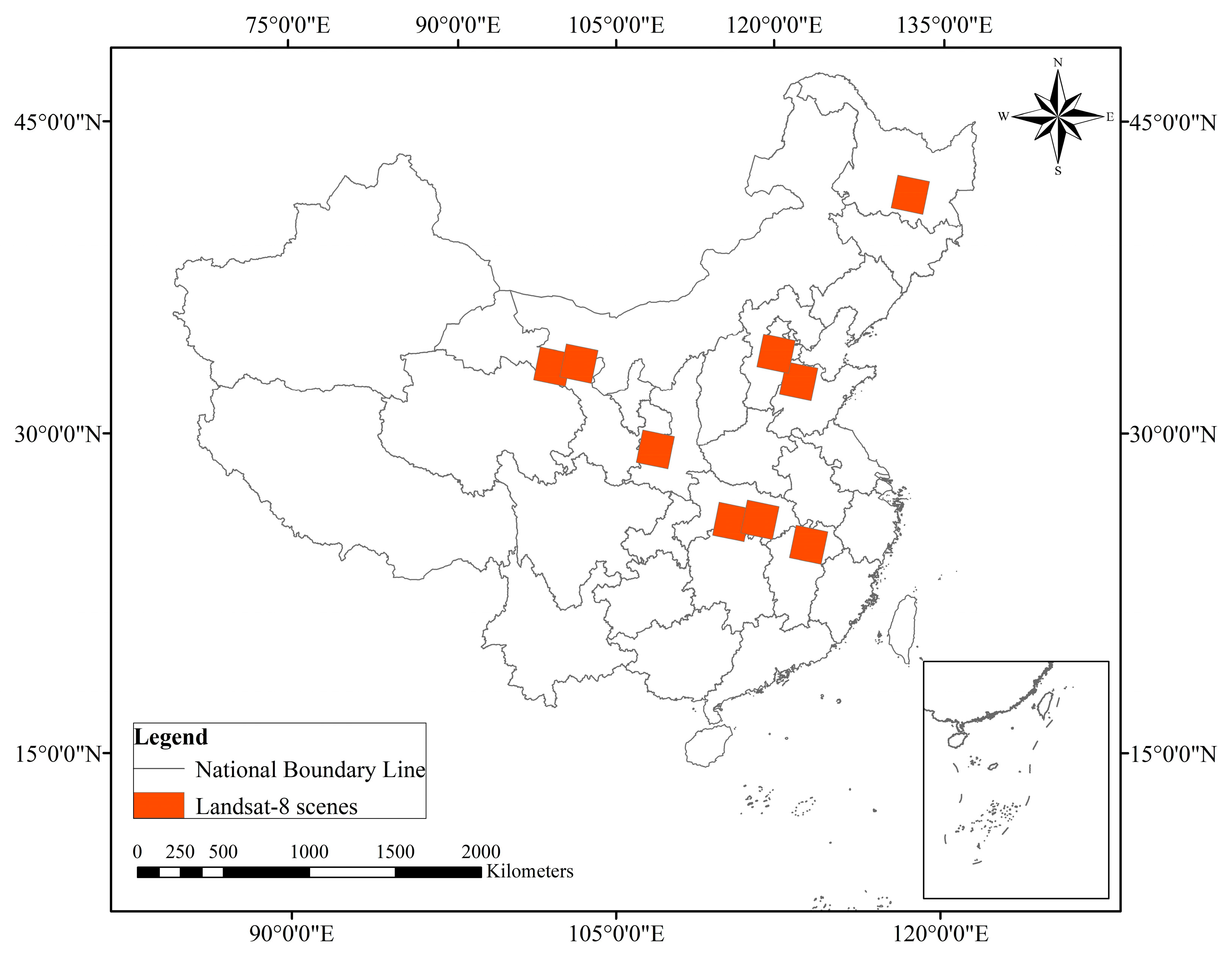
2.1. Study Areas

The study areas were located in northeast, north, central, southeast, and northwest China (Figure 1), where typical crops are grown. Three major crops (rice, wheat, and corn) are the principal resources regarding crop straw, and they comprise ~75% of the total straw production in China [35]. The areas of burning fires were identified according to the major grain-growing subregions. In line with the types and phenological characteristics of crops in the administrative subregions in China, the study areas were divided into three different types: “spring–autumn dominant”, “autumn–winter dominant”, and “summer–autumn dominant”.
Three areas of burning fires mainly occur during the crop harvesting season, which is from February to October, from September to March, from June to July, and from October to December, respectively, for the northeast, north, central, southeast, and northwest. The “spring–autumn dominant” areas are mainly in central and southeast China, the “autumn–winter dominant” areas are mainly in northern and northeast China, and the “summer–autumn dominant” areas are mainly in northwest China. The crops grown in these areas are mainly rapeseed in spring, rice in summer, and wheat in winter; corn and wheat in spring; or corn in summer and wheat in winter.

2.2. Data

2.2.1. Landsat-8 Images

The Landsat-8 satellite was designed by NASA and launched on 11 February 2013 into a sun-synchronous orbit at an altitude of 705 km with a 16-day revisit period. The Landsat-8 satellite carries the Operational Land Imager (OLI) and the Thermal Infrared Sensor (TRIS), and the OLI sensor has 30-m spatial resolution for Bands 1–7 and 9 and resolution of 15 m for the panchromatic band (Band 8) [36]. In this study, Landsat-8 OLI (L1T) data corrected for standard topography and geometry were converted to top-of-atmosphere (TOA) spectral reflectance using L1T calibration coefficients in the metadata (MTL) file.
Table 1 summarizes the acquisition time for and information about the nine chosen Landsat-8 images, which included three scenes each for “spring–autumn dominant”, “autumn–winter dominant”, and “summer–autumn dominant” areas. Figure 1 shows the locations of the selected Landsat-8 imagesin study areas, in which the images’ features include burning fires, burning areas, croplands, urban and rural buildings, etc. This image dataset contained image patches of 500 × 500 pixels, excluding the patches of the images covered with clouds, and it was extracted from Landsat-8 images between March 2016 and December 2018.

2.2.2. Burning Fires and Non-Fire Datasets

The dataset included burning fires and non-fire datasets, with the non-fire dataset including cropland vegetation, buildings, highly reflective buildings, and water. Table 2 shows the type and quantity of samples in the datasets. The ground truth (GT) data were composed of visual interpretations of 15-m images based on a fusion of Landsat-8 images, the locations of historically active fires, and information from a comparison based on Google Earth images acquired before and after the fires occurred. The locations and information of historically active fires were derived from the Satsee-Fire active fire detection system (http://satsee.radi.ac.cn:8080/index.html) of the Institute of Remote Sensing and Digital Earth Research, Chinese Academy of Sciences.
The ground truth (GT) dataset comprised 480 burning fires, 360 of which were used for training and testing and 120 for model validation. A burning fire was defined as a true active fire characterized by noticeable smoke from burning or a burning area. We determined and manually labeled burning fires in the Landsat-8 images from a combination of Band 7 (SWIR: 2.20 μm), Band 6 (SWIR: 1.61μm), and Band 4 (red: 0.66 μm) [26,36], combined with the true color B4–B3–B2 bands to form the ground truth ROI (region of interest). The coordinates of the burning fires were then saved for training and testing.

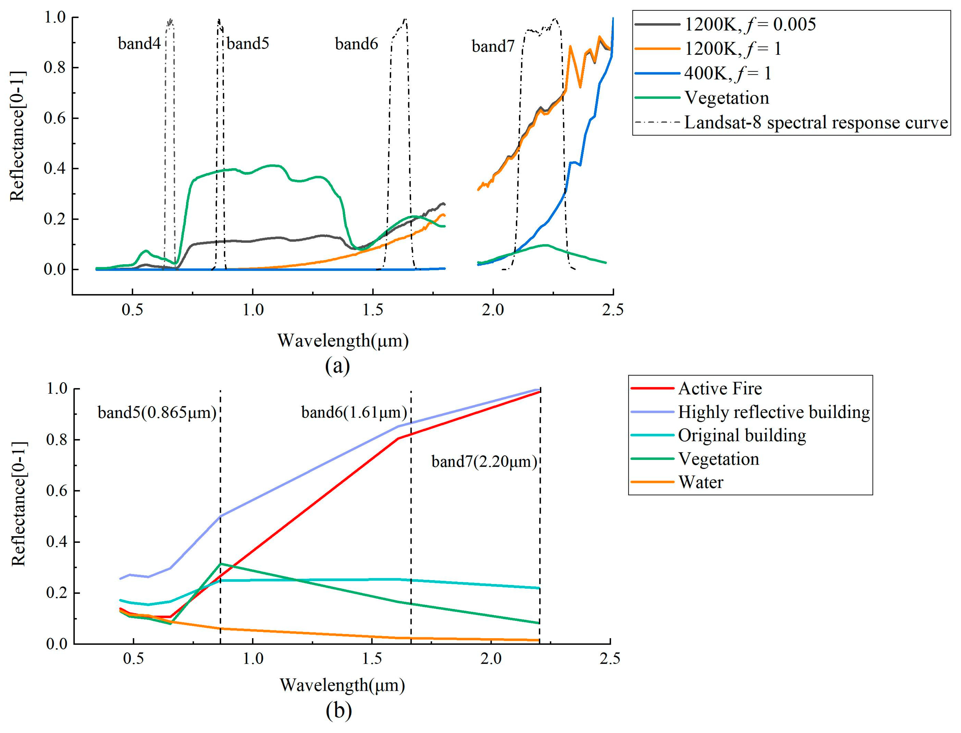
2.3. Spectral Analysis of Burning Fires

Planck’s law, the blackbody radiation law, is the basic theory behind active fire detection [25], and it defines the blackbody spectral emissivity on the basis of the blackbody temperature. The spectral radiance of the satellite observations of active fires is related to the temperature and size of the non-fire components [37]. When an active fire is smaller than the size of Landsat-8 pixels (30 m), the spectral radiance includes the non-fire component and the burning fire component. Planck’s law is defined as follows
B B ( λ , T ) = 2 h c 2 λ 5 · 1 ( e h c / λ k T 1 )
where B(λ, T) is the blackbody emitted radiance (W/sr/(m2∙m)), h (J∙s) is Planck’s constant, c (m/s) is the speed of light in a vacuum, and T (K) is the thermodynamic temperature.
Active fires were divided into smoldering and flaming phases. The typical temperatures of smoldering and flaming fires are about 400–500 K and 800–1200 K, respectively, with the specific temperature depending on the actual environmental conditions and components being burned [25,37]. The components of burning straw are dominated by crop straw. Typically, the areas of crop burn-offs are scattered and smaller than those of forest fires, and the intensity of burning may be smaller than the 30-m pixel dimension of Landsat-8 images [26].
Planck’s radiation equation allows us to simulate the spectral radiance and determine the spectral reflectance based on active fires with different temperatures and different pixel sizes, assuming that an active fire is an ideal blackbody (spectral emissivity = 1), neglecting the atmospheric conditions. The reflectivity of an active fire is negligible, and the spectral reflectance profile of an active fire can be simulated for different temperatures and sizes according to Equation (2) [26]
ρ s i m , λ = ( 1 f ) · ρ v e g , λ + f · B B ( λ , T ) E 0 , λ
where ρsim,λ is the simulated spectral reflectance corresponding to the wavelength λ, f is the spatial fraction [0–1] of the burning pixels, ρveg,λ is the spectral reflectance of the background vegetation, and E0,λ (W/sr/(m2∙m)) is the surface-level solar irradiance.
Figure 2a shows the simulated spectral reflectance profile [17,26] using typical spectra of vegetation as non-fire spectra. The spectral reflectance of active fires was simulated with different spatial fractions of the pixels (f), namely f = 0.005 and f = 1, when the temperature was 1200 K and 400 K, respectively. We assumed that, when the temperature was 1200 K, the spatial fraction of the pixel was f = 0.005 for small-scale burning fires, and the actual burning area occupied about 4.5 m2 of the Landsat-8 image.
It can be seen that, at the same temperature (1200 K), the extent of burning fires mainly affected the near-infrared variation in the reflectance, and the smaller the area of combustion was (f = 0.005), the more it was correlated with the reflectance characteristics of the background value [38]. At the same extent of burning fires (f = 1), the temperature of the fire mainly affected the change in the reflectance of the SWIR band (1.61 μm to 2.5 μm), and the higher temperature (1200 K) was more sensitive. Temperature variations have a strong influence on SWIR bands; in particular, B6 (1.61μm) and B7 (2.2 μm) of Landsat-8 are the sensitive and crucial band features for constructing the burning fire model [39].
To further understand the distinction between burning fires and the spectral reflectance of other typical features (Figure 2b), spectral statistics were collected from 50 samples of burning fires, water, original buildings, vegetation, and highly reflective buildings in the Landsat-8 imagery for the study area. The reflectance of burning fires is significantly different from that of typical land features except for highly reflective buildings. The trend of the spectral reflectance of highly reflective buildings is basically the same as that of burning fires, especially in B6 and B7, for which it is difficult to set the threshold. The burning fires in the range of the NIR bands were similar to the trend of the reflectance of vegetation, consistent with the reflectance of active fires and vegetation simulated in Figure 2a.

2.4. Methods

2.4.1. The SAFD Multicriteria Threshold Algorithm in the Context of Croplands

A crucial aspect of constructing the SAFD algorithm is determining the threshold between burning fires and non-fires. This algorithm was based on the advantages of the Landsat-8 GOLI algorithm proposed by [26] and the AFD-S2 algorithm proposed by [22]. According to the spectral analysis of burning fires presented in Section 2.3, the SAFD algorithm constructed a relational equation based on the B4, B6, and B7 Landsat-8 images.
The algorithm was based on three criteria (Equations (3)–(5)) and was divided into two steps. First, potential active fires were detected in the context of croplands by Equations (3) and (4) with the objective of marking as many fire pixels as possible. An OLS (ordinary least squares) regression was established using the B4 and B7 bands based on the cropland samples to determine the threshold (Equation (3)). Second, Equation (5) was constructed to further differentiate burning fires from non-fire pixels. The improved threshold reduced the interference of highly reflective buildings for detecting burning fires. The specific threshold was as determined in Section 3.1.
ρ 0.66 a · ρ 2.20 b
ρ 2.20 c
where ρ0.66 and ρ2.20 represent the Landsat-8 TOA reflectance of B4 and B7, respectively; the thresholds of a, b, and c are determined by the probability intervals; a and b are determined by the predicted lower 3σ standard deviation; and the value of c is determined by the 0.99 quantile, which is greater than or equal to the corresponding threshold.
ρ 2.20 / ρ 1.61 d   O R   ρ 1.61 e
where d represents the fixed thresholds. Note that d takes the value statistically determined by the spectral reflectance values of active fires and non-fires calculated by Equations (3) and (4), and e takes a value with reference to [22].

2.4.2. Constructing the Algorithm to Consider the Interference of Highly Reflective Buildings

The LightGBM machine learning algorithm was constructed to improve the problem of the high CE of the threshold methods for detecting burning fires in urban and rural areas. The LightGBM (light gradient boosting machine) algorithm is a GBDT framework based on the decision tree algorithm proposed by Microsoft Research Asia (2017). That research used the GOSS (gradient-based one-side sampling) and EFB (exclusive feature bundling) methods to improve the limitations of the GBDT algorithm with the aims of reducing the samples and features, respectively. The LightGBM algorithm performs better with multidimensional features and can construct classification rules based on fewer samples. It is more suitable for models with smaller samples than neural networks or some other machine learning methods, and it was used to detect burning fires in this study.
This method focused on selecting the features of active fires and buildings using the ReliefF method for selecting a combination of features. We initially extracted 25 features of burning fires and buildings (Table 3), including the original bands (Band 1 to Band 7), a spectral index (NDBI) [40], NDVI, NBR [41], and the textural features (mean, variance, standard deviation, homogeneity, contrast, and correlation) of B4, B6, and B7.
The texture features were selected via the gray-level co-occurrence matrix (GLCM) [42]. The basic aim was to calculate the co-occurrence frequency of the pixel values in the sliding window and then to extract the characteristics of the co-occurrence matrix via various statistical measures. The texture features were calculated using a 3 × 3 sliding window, and the formula is shown in Table 3.

2.4.3. Evaluation Metrics

The algorithm’s detections were evaluated by their accuracy, based on the confusion matrix (Table 4) compared with the GT dataset. Five indicators of accuracy, namely precision (P), recall, commission errors (CE), omission errors (OE), and the evaluation index (F), were computed via Equations (6)–(10) [43]. Precision and recall are defined as the ratio of the correct targets detected to the number of detected targets and the ratio of correctly detected targets to the actual number of targets, respectively. The higher the precision and recall, the more accurate the detection.
P = T P T P + F P
R e c a l l = T P T P + F N
C E = F P T P + F P
O E = F N T P + F N
F = 2 P ( 1 O E ) 1 + P O E
where TP represents the true positive predictions of active fire pixels; TN represents the true negative predictions of active fire pixels, indicating correctly labeled non-fires; FP represents non-fire pixels that were predicted to be active fires; and FN represents active fire pixels incorrectly labeled as non-fires.

3. Results

3.1. Specifying the Threshold of the Multicriteria SAFD Algorithm

The threshold range of potential burning fires was specified on the basis of 1712 cropland samples using random sampling with 30-m landcover products (http://www.webmap.cn). The samples’ locations were uniformly distributed in the study area. Figure 3 shows the scatterplot of the range of potential burning fires. The scatterplots correspond to the Landsat-8 TOA reflectance in the B4 and B7 bands. The fitted curve (blue line) of the OLS regression for cropland samples showed a significant relationship, as the coefficient of determination (R2) was 0.56 due to the differences in the croplands’ vegetation types. The threshold range of potential active fires was determined by Equations (11) and (12). When a point was within this threshold range, it was considered to be a potential active fire.
B 4 0.4731 B 7 0.0147
B 7 0.267
The statistical histogram for the thresholds specified for d and e is displayed in Figure 4. Samples were selected on the basis of the threshold range of potential active fires, with totals of 960 and 480 active fire samples and non-fire samples, respectively. As shown in Figure 4, the red dashed line is the dividing line in the interval of 2–2.2. The correct rate of active fires showed a rapidly increasing trend of 77.78%, and the correct rate increased and tended to become stable after the interval of 2.2–2.4. In the algorithms proposed by [19,28], the ratios of ρ2.20 and ρ1.61 took values of 1.4 and 1.6, respectively, and these values had high CE in urban and rural areas. Therefore, the fixed threshold of burning fires in urban and rural areas was 2. Equation (13) is as follows
ρ 2.20 / ρ 1.61 2   OR   ρ 1.61 1

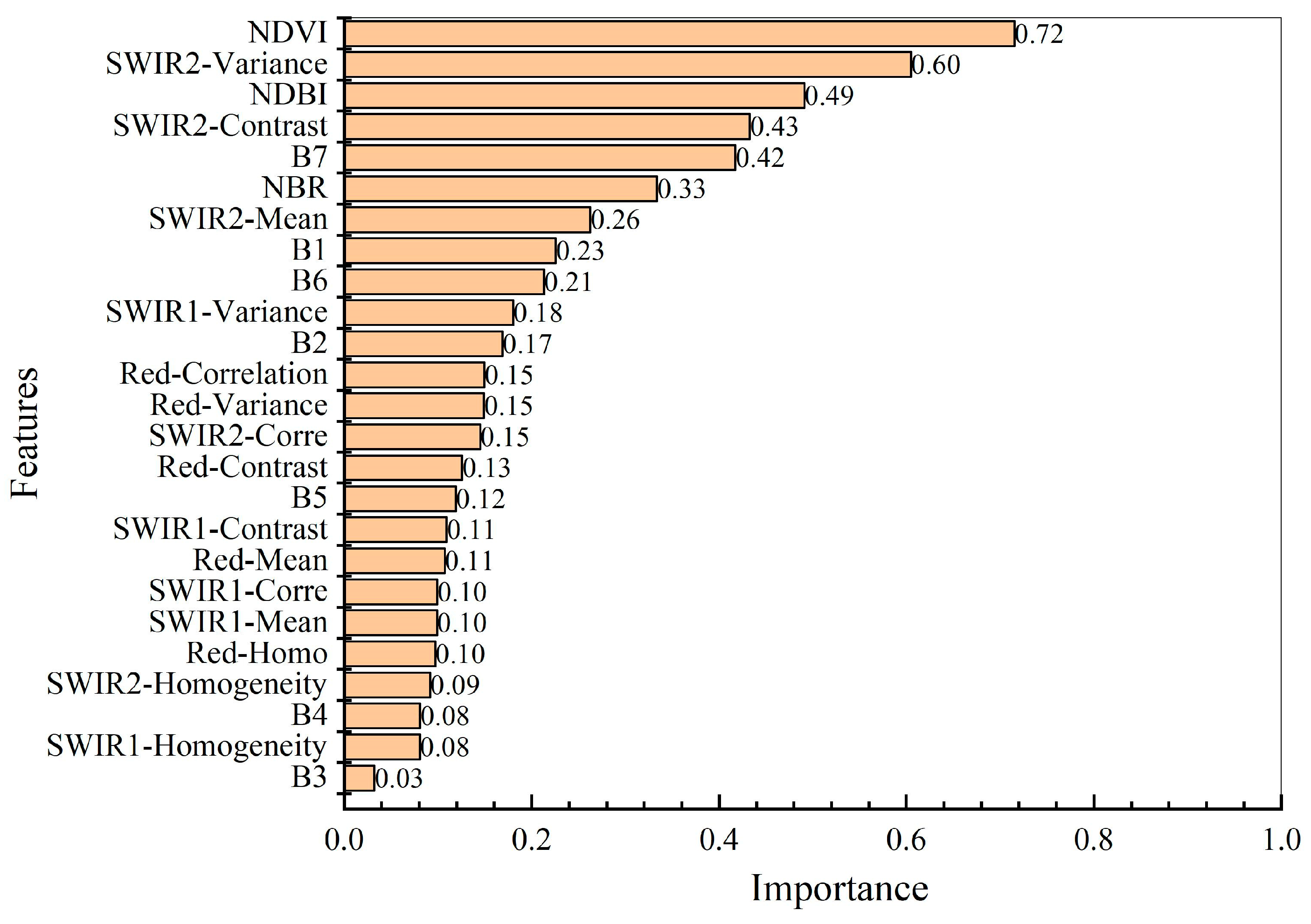
3.2. Selection of the Features’ Variables via the SAFD-LightGBM Model

To consider the effects of highly reflective buildings on the detection of burning fires, a total of 1580 training samples were used, of which 360 were positive samples of active fires, and 1220 buildings were misclassification samples. Regarding the imbalance between the samples of burning fires and non-fires [44], Logloss was used as the objective function, and the weight parameter scale_pos_weight was optimized by the GridSearch-CV hyperparameter selection method. The optimal weight parameter for constructing the SAFD-LightGBM model was 0.3.
Figure 5 shows the importance of the ReliefF method for each feature, where the spectral index features NDVI, NDBI, and NBR were ranked among the top 10 features. The NDVI index is a reference for burning fires that ranked first among all the features [45]. The texture features of the variance and contrast of B7 (SWIR2) contributed significantly to the detection of burning fires. The backward selection method was used to find the optimal combination of features. The optimal combination of features was 10 selected features. The recall and precision were 0.93 and 97%, respectively, and the F1 score was 0.95. The results of validating the model for various iterations are shown in Figure 6. In total, 100 iterations of model validation were performed, and it can be noted that the variation in Logloss appeared to be low and fluctuated slightly from Iterations 55 to 60.

3.3. Comparison of the SAFD and SAFD-LightGBM Algorithms

3.3.1. Analysis of the Results of Detecting Burning Fires

Figure 7 shows a comparison of the results with each algorithm for Scenes a and b. Scene a is a burning fire in a rural area, with more obvious smoke from burning. Scene b is a burning fire in an urban area, with which smoke is not apparent, and the burning area is prominent. Position a in Scenes a and b represents the location where the burning fire occurred, and Positions b to f indicate locations of false detections.
It can be seen that the results of SAFD for Scene a had five burning fire pixels, while the results for SAFD-LightGBM showed four fire pixels. SAFD identified six fire pixels in Scene b, and SAFD-LightGBM missed some fire pixels around the burning area because the smoke obscured the burning fire, resulting in weak penetration or affecting the ability to detect smoldering fires. Second, the scenes were analyzed against a mixed crop background spectrally due to the high-temperature burning fires with very small fractional areas (f < 0.01, that is, 9 m2). The spectra fitted well for pixels that contained a relatively larger fractional area of smoldering fire and cropland (Figure 2) [38]. Nevertheless, SAFD-LightGBM had little influence on the locations of burning fires or the information acquired.
On the other hand, highly reflective buildings interfere substantially with the process of detecting burning fires. The misclassified pixels are scattered in Scenes a and b, and the anomalies on the buildings’ rooftops significantly increased the CE of the SAFD, mainly due to the threshold, which mostly considered the relationship of the critical bands and could not completely differentiate the buildings from the burning fires. The results of SAFD-LightGBM showed that the pixels of highly reflective buildings were effectively eliminated in Scene a and reduced in Scene b.
The misclassified highly reflective buildings were divided into three categories to further discuss the algorithms’ results (Figure 8). Figure 8a shows the false flame that was generated during the production or operation of factories. Figure 8b shows that the false fire was on a stadium roof. Figure 8c shows the false detection of the rooftops of single or multiple discrete buildings. The SAFD algorithm in urban and rural areas generated a large CE, consistent with the findings of previous studies [19,26,28]. The results showed that SAFD-LightGBM performed better than SAFD, especially for the suspected flames generated by factories due to their operations.

3.3.2. Accuracy Validation

Three scenes (WRS: 117/28, 128/36, 121/40) (Table 1) with a total of 120 burning fires were used to evaluate the algorithms. Figure 9 shows the scatterplot of both algorithms’ results. This plot revealed that some misclassified pixels of highly reflective buildings in SAFD’s results were distributed on the threshold edge of  ρ 2.20 / ρ 1.61 2  in Figure 9c. The results of SAFD-LightGBM found that most of the misclassifications were eliminated, as shown in Figure 9e. Table 5 shows a comparison of the accuracy of the algorithms. In terms of CE and OE, SAFD had a low CE and a high OE of 8.9% and 29.0%, respectively. While the CE of the SAFD-LightGBM was 15.8% lower, the OE was higher relative to those of the SAFD algorithm. The SAFD-LightGBM algorithm had a better balance between the OE and the CE. The accuracy (P) was 86.8%, and the comprehensive evaluation index (F) was 87.6, which was 7.8% higher and better than that of the SAFD algorithm.

4. Discussion

4.1. Comparison of Commission Errors in Different Regions

The CEs of both algorithms were used to further analyze the applicability in study areas with different dominant seasons, as shown in Figure 10. The SAFD and SAFD-LightGBM algorithms had the lowest CE in the “summer–autumn dominant” regions. The highest CEs in the “spring–autumn dominant” regions were 38.7% and 24.5%, respectively, for SAFD and SAFD-LightGBM. A high CE was found for the “spring–autumn dominant” regions located in the eastern and central regions of China, where many major agricultural provinces have a high degree of rural agglomeration and rich cropland resources that may cause potential misclassifications of pixels during burning [46,47]. In contrast, the “summer–autumn dominated” areas are located in northwestern China, which has a dry climate, low vegetation cover, a single crop type, and a transparent partition between urban and rural areas and arable crop areas. The SAFD-LightGBM algorithm had a significantly improved CE in the “summer–autumn dominated” area, which was reduced by 16.81%. The algorithm could also be applied in similar areas, especially in “summer–autumn dominated” areas.

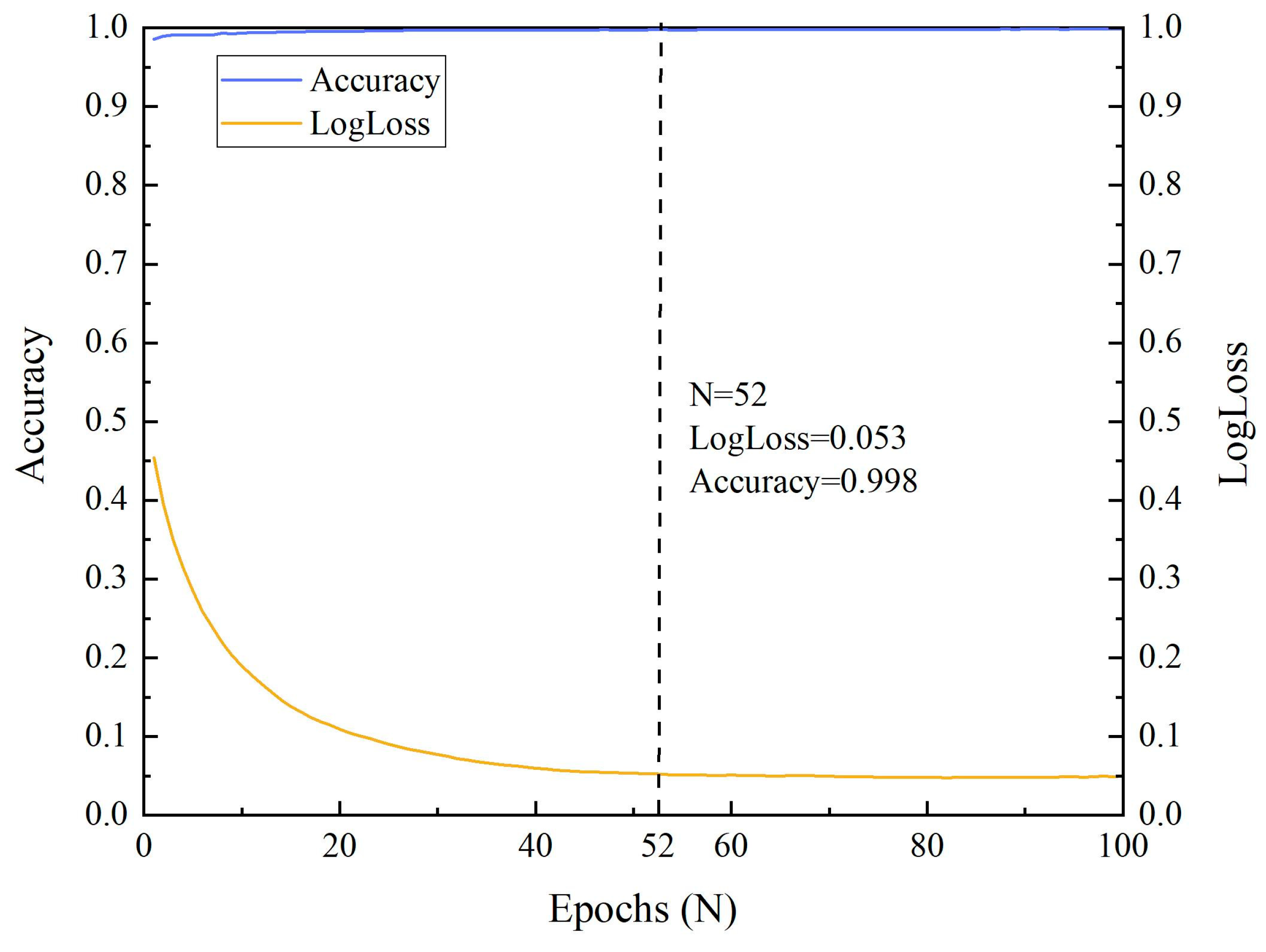
4.2. Influence of Hyperparameter Adjustment on the Model

To investigate the effect of parameter selection on the results, we performed hyperparameter optimization of the model. The key parameters of the model, namely learning rate, n_estimators and num_leaves, were selected, and their effects on the model were observed by setting different intervals (Table 6, Figure 6). It can be seen that the improvement in the model by setting different intervals of learning_rate is not obvious (Figure 11a). Further, the n_estimators and num_leaves parameters showed significant improvement. The model tended to be stable when n_estimators was in the range of 150–200, and the model performance was no longer significant when n_estimators ≥ 200. Meanwhile, the model performance was better when num_leaves was in the range of 25–45. The model results of optimized parameters showed that OE and CE were 11.5% and 13.2%, respectively.

4.3. Advantages and Limitations of the SAFD-LightGBM Algorithm

The influence of highly reflective buildings on the detection of active fires has been widely discussed by researchers [26,28,48]. Our method highlights the ability of machine learning to discriminate between highly reflective buildings and burning fires. One difficulty with the current methods of monitoring small-scale fires is that OEs are usually caused by small and cool fires, and CEs are likely to occur in soil-dominated pixels or the highly reflective rooftops of buildings [49,50]. A second difficulty is that the occurrence, location, and information of fire pixels are randomly changing and are disturbed by a large amount of background information during the period, and the proportions of the active fire and the background pixels are unbalanced [49]. The proposed statistics-based algorithm can consider burning fires as a linear process of removing the background information, leaving the potential fire information, which can improve the quality of the machine learning algorithm. However, the statistical approach has some limitations in its generalizability, and there have been studies showing that specific vegetation environments have different effects on active fires [51,52], so the statistics-based algorithm combined with machine learning method should mainly be used for detecting small-scale fires in croplands, which are of considerable significance.

5. Conclusions

We proposed the SAFD-LightGBM algorithm to improve the problem of the high CE of the threshold method in urban and rural areas. The SAFD-LightGBM algorithm is a feasible solution to the problem of reducing the influence of highly reflective buildings on the detection of burning fires. It can also reduce the false positives caused by buildings while ensuring the accuracy of detecting burning fires as much as possible. The algorithm has stability and applicability for discrete burning fires in urban and rural areas.
  • Based on the statistical samples, a multicriteria threshold method was constructed to eliminate the background pixels of the cropland. Burning fires were then accurately extracted from the dataset of potential fires and other non-fires. It was found that the proposed improved threshold model was mainly influenced by the buildings around urban and rural areas, with detection precision of 71%.
  • We used machine learning to accurately detect burning fires and found that the texture features of variance and contrast made a greater contribution to distinguishing fires from non-fires, and the precision of the algorithm in terms of the texture features was 86.8%. We ran the algorithm for different regions and found that the improved algorithm had the highest precision of 96.91% in summer–autumn dominant regions.
  • For detecting small burning fires, in most regions, the majority of false fire pixels were linked to clusters of true fire pixels, suggesting that most false fire pixels occur along the ambiguous boundaries of fires. This phenomenon occurred more in northeastern China.
The application of this method could be promoted by further experiments with more medium- and high-resolution sensors without thermal infrared bands and by combining the method with images from other satellites with different resolutions and periods (e.g., Landsat-8 combined with Sentinel-2 and Landsat-9 satellites). Presently, the pollutants emitted from burning fires remain the dominant source of air pollution. The next step will be a more targeted exploration of the construction of a high-quality and reliable sample set for detecting burning fires to improve the applicability and reliability of the algorithm.

Author Contributions

Conceptualization, J.K. and Y.J.; methodology, J.K. and Y.J.; software, Y.J.; validation, Y.J. formal analysis, J.K. and Y.J.; investigation, Y.J. and Q.Z.; resources, Y.J. and Y.Z.; data curation, Y.J. and Q.Z.; writing—original draft, Y.J. and Y.Z.; writing—review and editing, Y.J. and J.Z.; visualization, Y.J. and J.Z.; supervision, J.K.; project administration, J.K.; funding acquisition, J.K. All authors have read and agreed to the published version of the manuscript.

Funding

This work was supported by the Department of Science and Technology of Shaanxi Province’s key research and development projects (2020ZDLSF06-07).

Data Availability Statement

All data in this article can be obtained by contacting the corresponding author.

Acknowledgments

The authors thank the Institute of Remote Sensing and Digital Earth of the Chinese Academy of Sciences for the near real-time surface high temperature anomalies and information about active fires from the SatSee-Fire (Satellite See Fire) service system.

Conflicts of Interest

The authors declare no conflict of interest.

References

  1. Ayala-Carrillo, M.; Farfán, M.; Cárdenas-Nielsen, A.; Lemoine-Rodríguez, R. Are Wildfires in the Wildland-Urban Interface Increasing Temperatures? A Land Surface Temperature Assessment in a Semi-Arid Mexican City. Land 2022, 11, 2105. [Google Scholar] [CrossRef]
  2. Li, J.; Bo, Y.; Xie, S. Estimating Emissions from Crop Residue Open Burning in China Based on Statistics and MODIS Fire Products. J. Environ. Sci. 2016, 44, 158–170. [Google Scholar] [CrossRef] [PubMed]
  3. Frolking, S.; Xiao, X.; Zhuang, Y.; Salas, W.; Li, C. Agricultural Land-Use in China: A Comparison of Area Estimates from Ground-Based Census and Satellite-Borne Remote Sensing. Glob. Ecol. Biogeogr. 1999, 8, 407–416. [Google Scholar] [CrossRef] [Green Version]
  4. Xiao, X.; Liu, J.; Zhuang, D.; Frolking, S.; Boles, S.; Xu, B.; Liu, M.; Salas, W.; Moore, B., III; Li, C. Uncertainties in Estimates of Cropland Area in China: A Comparison between an AVHRR-Derived Dataset and a Landsat TM-Derived Dataset. Glob. Planet. Chang. 2003, 37, 297–306. [Google Scholar] [CrossRef]
  5. Streets, D.G.; Yarber, K.F.; Woo, J.-H.; Carmichael, G.R. Biomass Burning in Asia: Annual and Seasonal Estimates and Atmospheric Emissions. Glob. Biogeochem. Cycles 2003, 17, 1759–1768. [Google Scholar] [CrossRef] [Green Version]
  6. Liu, M.; Song, Y.; Yao, H.; Kang, Y.; Li, M.; Huang, X.; Hu, M. Estimating Emissions from Agricultural Fires in the North China Plain Based on MODIS Fire Radiative Power. Atmos. Environ. 2015, 112, 326–334. [Google Scholar] [CrossRef]
  7. Zhang, H.; Hu, J.; Qi, Y.; Li, C.; Chen, J.; Wang, X.; He, J.; Wang, S.; Hao, J.; Zhang, L.; et al. Emission Characterization, Environmental Impact, and Control Measure of PM2.5 Emitted from Agricultural Crop Residue Burning in China. J. Clean. Prod. 2017, 149, 629–635. [Google Scholar] [CrossRef]
  8. Prins, E.M.; Menzel, W.P. Geostationary Satellite Detection of Bio Mass Burning in South America. Int. J. Remote Sens. 1992, 13, 2783–2799. [Google Scholar] [CrossRef]
  9. Elvidge, C.; Ziskin, D.; Baugh, K.; Tuttle, B.; Ghosh, T.; Pack, D.; Erwin, E.; Zhizhin, M. A Fifteen Year Record of Global Natural Gas Flaring Derived from Satellite Data. Energies 2009, 2, 595–622. [Google Scholar] [CrossRef] [Green Version]
  10. Böhme, C.; Bouwer, P.; Prinsloo, M.J. Real-Time Stream Processing for Active Fire Monitoring on Landsat 8 Direct Reception Data. Int. Arch. Photogramm. Remote Sens. Spat. Inf. Sci. 2015, XL-7/W3, 765–770. [Google Scholar] [CrossRef] [Green Version]
  11. Jiang, L.; Du, W.; Yu, S. Estimation of Heat Released from Fire Based on Combustible Load in Inner Mongolian Grasslands. Land 2022, 11, 2099. [Google Scholar] [CrossRef]
  12. Elvidge, C.; Zhizhin, M.; Hsu, F.-C.; Baugh, K. VIIRS Nightfire: Satellite Pyrometry at Night. Remote Sens. 2013, 5, 4423–4449. [Google Scholar] [CrossRef] [Green Version]
  13. Giglio, L.; Schroeder, W.; Justice, C.O. The Collection 6 MODIS Active Fire Detection Algorithm and Fire Products. Remote Sens. Environ. 2016, 178, 31–41. [Google Scholar] [CrossRef] [Green Version]
  14. Stroppiana, D.; Pinnock, S.; Gregoire, J.-M. The Global Fire Product: Daily Fire Occurrence from April 1992 to December 1993 Derived from NOAA AVHRR Data. Int. J. Remote Sens. 2000, 21, 1279–1288. [Google Scholar] [CrossRef]
  15. Schroeder, W.; Oliva, P.; Giglio, L.; Csiszar, I.A. The New VIIRS 375 M Active Fire Detection Data Product: Algorithm Description and Initial Assessment. Remote Sens. Environ. 2014, 143, 85–96. [Google Scholar] [CrossRef]
  16. Wooster, M.J.; Xu, W.; Nightingale, T. Sentinel-3 SLSTR Active Fire Detection and FRP Product: Pre-Launch Algorithm Development and Performance Evaluation Using MODIS and ASTER Datasets. Remote Sens. Environ. 2012, 120, 236–254. [Google Scholar] [CrossRef]
  17. Giglio, L.; Descloitres, J.; Justice, C.O.; Kaufman, Y.J. An Enhanced Contextual Fire Detection Algorithm for MODIS. Remote Sens. Environ. 2003, 87, 273–282. [Google Scholar] [CrossRef]
  18. Wright, R.; Flynn, L.P.; Garbeil, H.; Harris, A.J.L.; Pilger, E. MODVOLC: Near-Real-Time Thermal Monitoring of Global Volcanism. J. Volcanol. Geotherm. Res. 2004, 135, 29–49. [Google Scholar] [CrossRef]
  19. Murphy, S.W.; de Souza Filho, C.R.; Wright, R.; Sabatino, G.; Correa Pabon, R. HOTMAP: Global Hot Target Detection at Moderate Spatial Resolution. Remote Sens. Environ. 2016, 177, 78–88. [Google Scholar] [CrossRef]
  20. USGS Landsat 8 Data Users Handbook. Available online: https://landsat.usgs.gov/documents/Landsat8DataUsersHandbook.pdf. (accessed on 27 November 2019).
  21. Drusch, M.; Del Bello, U.; Carlier, S.; Colin, O.; Fernandez, V.; Gascon, F.; Hoersch, B.; Isola, C.; Laberinti, P.; Martimort, P.; et al. Sentinel-2: ESA’s Optical High-Resolution Mission for GMES Operational Services. Remote Sens. Environ. 2012, 120, 25–36. [Google Scholar] [CrossRef]
  22. Hu, X.; Ban, Y.; Nascetti, A. Sentinel-2 MSI Data for Active Fire Detection in Major Fire-Prone Biomes: A Multi-Criteria Approach. Int. J. Appl. Earth Obs. Geoinf. 2021, 101, 102347. [Google Scholar] [CrossRef]
  23. Li, J.; Roy, D.P. A Global Analysis of Sentinel-2A, Sentinel-2B and Landsat-8 Data Revisit Intervals and Implications for Terrestrial Monitoring. Remote Sens. 2017, 9, 902. [Google Scholar] [CrossRef] [Green Version]
  24. Csiszar, I.A.; Schroeder, W. Short-Term Observations of the Temporal Development of Active Fires from Consecutive Same-Day ETM+ and ASTER Imagery in the Amazon: Implications for Active Fire Product Validation. IEEE J. Sel. Top. Appl. Earth Observ. Remote Sens. 2008, 1, 248–253. [Google Scholar] [CrossRef]
  25. Giglio, L.; Csiszar, I.; Restás, Á.; Morisette, J.T.; Schroeder, W.; Morton, D.; Justice, C.O. Active Fire Detection and Characterization with the Advanced Spaceborne Thermal Emission and Reflection Radiometer (ASTER). Remote Sens. Environ. 2008, 112, 3055–3063. [Google Scholar] [CrossRef]
  26. Kumar, S.S.; Roy, D.P. Global Operational Land Imager Landsat-8 Reflectance-Based Active Fire Detection Algorithm. Int. J. Digit. Earth 2017, 11, 154–178. [Google Scholar] [CrossRef] [Green Version]
  27. Schroeder, W.; Prins, E.; Giglio, L.; Csiszar, I.; Schmidt, C.; Morisette, J.; Morton, D. Validation of GOES and MODIS Active Fire Detection Products Using ASTER and ETM+ Data. Remote Sens. Environ. 2008, 112, 2711–2726. [Google Scholar] [CrossRef]
  28. Schroeder, W.; Oliva, P.; Giglio, L.; Quayle, B.; Lorenz, E.; Morelli, F. Active Fire Detection Using Landsat-8/OLI Data. Remote Sens. Environ. 2016, 185, 210–220. [Google Scholar] [CrossRef] [Green Version]
  29. De Almeida Pereira, G.H.; Fusioka, A.M.; Nassu, B.T.; Minetto, R. Active Fire Detection in Landsat-8 Imagery: A Large-Scale Dataset and a Deep-Learning Study. ISPRS J. Photogramm. Remote Sens. 2021, 178, 171–186. [Google Scholar] [CrossRef]
  30. Wooster, M.J.; Roberts, G.J.; Giglio, L.; Roy, D.; Freeborn, P.; Boschetti, L.; Justice, C.; Ichoku, C.; Schroeder, W.; Davies, D.; et al. Satellite Remote Sensing of Active Fires: History and Current Status, Applications and Future Requirements. Remote Sens. Environ. 2021, 267, 112694. [Google Scholar] [CrossRef]
  31. Rostami, A.; Shah-Hosseini, R.; Asgari, S.; Zarei, A.; Aghdami-Nia, M.; Homayouni, S. Active Fire Detection from Landsat-8 Imagery Using Deep Multiple Kernel Learning. Remote Sens. 2022, 14, 992. [Google Scholar] [CrossRef]
  32. Corradino, C.; Amato, E.; Torrisi, F.; Del Negro, C. Data-Driven Random Forest Models for Detecting Volcanic Hot Spots in Sentinel-2 MSI Images. Remote Sens. 2022, 14, 4370. [Google Scholar] [CrossRef]
  33. Huang, Y.F.; Xu, J.; Li, Z.H.; Zhang, J. A Fire Detection Algorithm Based on Machine Learning. Sci. Surv. Mapping 2020, 45, 64–70. [Google Scholar] [CrossRef]
  34. Mateo-García, G.; Laparra, V.; López-Puigdollers, D.; Gómez-Chova, L. Transferring Deep Learning Models for Cloud Detection between Landsat-8 and Proba-V. ISPRS J. Photogramm. Remote Sens. 2020, 160, 1–17. [Google Scholar] [CrossRef]
  35. Chen, J.; Li, C.; Ristovski, Z.; Milic, A.; Gu, Y.; Islam, M.S.; Wang, S.; Hao, J.; Zhang, H.; He, C.; et al. A Review of Biomass Burning: Emissions and Impacts on Air Quality, Health and Climate in China. Sci. Total Environ. 2017, 579, 1000–1034. [Google Scholar] [CrossRef] [Green Version]
  36. Roy, D.P.; Wulder, M.A.; Loveland, T.R.; Woodcock, C.E.; Allen, R.G.; Anderson, M.C.; Helder, D.; Irons, J.R.; Johnson, D.M.; Kennedy, R.; et al. Landsat-8: Science and Product Vision for Terrestrial Global Change Research. Remote Sens. Environ. 2014, 145, 154–172. [Google Scholar] [CrossRef] [Green Version]
  37. Elvidge, C.D.; Zhizhin, M.; Hsu, F.-C.; Baugh, K.; Khomarudin, M.R.; Vetrita, Y.; Sofan, P.; Suwarsono; Hilman, D. Long-Wave Infrared Identification of Smoldering Peat Fires in Indonesia with Nighttime Landsat Data. Environ. Res. Lett. 2015, 10, 065002. [Google Scholar] [CrossRef] [Green Version]
  38. Waigl, C.F.; Prakash, A.; Stuefer, M.; Verbyla, D.; Dennison, P. Fire Detection and Temperature Retrieval Using EO-1 Hyperion Data over Selected Alaskan Boreal Forest Fires. Int. J. Appl. Earth Obs. Geoinf. 2019, 81, 72–84. [Google Scholar] [CrossRef]
  39. Kato, S.; Miyamoto, H.; Amici, S.; Oda, A.; Matsushita, H.; Nakamura, R. Automated Classification of Heat Sources Detected Using SWIR Remote Sensing. Int. J. Appl. Earth Obs. Geoinf. 2021, 103, 102491. [Google Scholar] [CrossRef]
  40. Sánchez Sánchez, Y.; Martínez Graña, A.; Santos-Francés, F. Remote Sensing Calculation of the Influence of Wildfire on Erosion in High Mountain Areas. Agronomy 2021, 11, 1459. [Google Scholar] [CrossRef]
  41. Stankova, N.; Nedkov, R. Monitoring Forest Regrowth with Different Burn Ssverity Using Aerial and Landsat Data. IEEE Int. Geosci. Remote Sens. Symp. 2015, 6, 26–31. [Google Scholar]
  42. Adhikari, A.; Garg, R.D.; Pundir, S.K.; Singhal, A. Delineation of Agricultural Fields in Arid Regions from Worldview-2 Datasets Based on Image Textural Properties. Env. Monit. Assess. 2023, 195, 605. [Google Scholar] [CrossRef] [PubMed]
  43. Li, K.; Wang, B. DAR-Net: Dense Attentional Residual Network for Vehicle Detection in Aerial Images. Computation. Intell. Neurosci. 2021, 2021, 19. [Google Scholar] [CrossRef] [PubMed]
  44. Santi, E.; Clarizia, M.P.; Comite, D.; Dente, L.; Guerriero, L.; Pierdicca, N. Detecting Fire Disturbances in Forests by Using GNSS Reflectometry and Machine Learning: A Case Study in Angola. Remote Sens. Environ. 2022, 270, 112878. [Google Scholar] [CrossRef]
  45. Michael, Y.; Helman, D.; Glickman, O.; Gabay, D.; Brenner, S.; Lensky, I.M. Forecasting Fire Risk with Machine Learning and Dynamic Information Derived from Satellite Vegetation Index Time-Series. Sci. Total Environ. 2021, 764, 142844. [Google Scholar] [CrossRef]
  46. Wu, J.; Kong, S.; Wu, F.; Cheng, Y.; Zheng, S.; Yan, Q.; Zheng, H.; Yang, G.; Zheng, M.; Liu, D.; et al. Estimating the Open Biomass Burning Emissions in Central and Eastern China from 2003 to 2015 Based on Satellite Observation. Atmos. Chem. Phys. 2018, 18, 11623–11646. [Google Scholar] [CrossRef] [Green Version]
  47. Zhang, Y.; Sun, B.; Xiao, Y.; Xiao, R.; Wei, Y. Feature Augmentation for Imbalanced Classification with Conditional Mixture WGANs. Signal Process. Image Commun. 2019, 75, 89–99. [Google Scholar] [CrossRef]
  48. Liu, Y.; Zhi, W.; Xu, B.; Xu, W.; Wu, W. Detecting High-Temperature Anomalies from Sentinel-2 MSI Images. ISPRS J. Photogramm. Remote Sens. 2021, 177, 175–193. [Google Scholar] [CrossRef]
  49. Zhang, Q.; Ge, L.; Zhang, R.; Metternicht, G.I.; Liu, C.; Du, Z. Towards a Deep-Learning-Based Framework of Sentinel-2 Imagery for Automated Active Fire Detection. Remote Sens. 2021, 13, 4790. [Google Scholar] [CrossRef]
  50. Palacios, A.; Muñoz, M.; Darbra, R.; Casal, J. Thermal Radiation from Vertical Jet Fires. Fire Saf. J. 2012, 51, 93–101. [Google Scholar] [CrossRef]
  51. Lasaponara, R.; Abate, N.; Fattore, C.; Aromando, A.; Cardettini, G.; Fonzo, M.D. On the Use of Sentinel-2 NDVI Time Series and Google Earth Engine to Detect Land-Use/Land-Cover Changes in Fire-Affected Areas. Remote Sens. 2022, 14, 4723. [Google Scholar] [CrossRef]
  52. Nolè, A.; Rita, A.; Spatola, M.F.; Borghetti, M. Biogeographic Variability in Wildfire Severity and Post-Fire Vegetation Recovery across the European Forests via Remote Sensing-Derived Spectral Metrics. Sci. Total Environ. 2022, 823, 153807. [Google Scholar] [CrossRef] [PubMed]
Figure 1. Location of the Landsat-8 images used in this study.
Land 12 01246 g001
Figure 2. (a) Simulated reflectance spectra of active fires. (b) The difference between the spectral reflectance of active burning fires and typical land features from Landsat-8 in the study area.
Land 12 01246 g002
Figure 3. Scatterplot of the range of potential active fires in the context of croplands. The blue line shows the OLS regression, and the green, dashed line represents the predicted range based on the lower 3σ predicted by the OLS regression. The dashed vertical lines represent the thresholds derived via Equation (13). The bottom-right range between the dash-dotted line and the dashed vertical line is the range of possible active fire pixels. The histogram on the right represents the density in the bands (B4 and B7), where red represents greater density.
Land 12 01246 g003
Figure 4. Histogram of ratio of the TOA reflectance of B7 and B6 (the horizontal axis represents the TOA reflectance value of B7/B6 with an interval of 0.2, the red dashed line represents the threshold for distinguishing fire from non-fire. The left-hand y-axis represents the frequency of the reflectance, and the right-hand y-axis indicates the correct rate of true active fires in the range of the horizontal coordinates). The line graph corresponds to the correct percentage of active fires within the interval.
Land 12 01246 g004
Figure 5. Importance of the ReliefF feature selection method.
Land 12 01246 g005
Figure 6. Validation of Logloss and accuracy for the SAFD-LightGBM. The lowest Logloss and the highest accuracy were seen for N = 52.
Land 12 01246 g006
Figure 7. Comparison between the SAFD algorithm and the SAFD-LigthtGBM algorithm. (a) A burning fire in a rural area. (b) A burning fire in an urban area. Red pixels are the results predicted by the detection algorithms, the bright blue boxes represent results that detected the burning fires (marked as position a), and the yellow boxes represent false detections caused by highly reflective buildings (marked as position b to f).
Land 12 01246 g007
Figure 8. False detection results of different types of highly reflective buildings: (a) factories; (b) a large stadium; (c) residential buildings. The red boxes indicates the locations of the anomalies, the bright blue pixels represent the highly reflective buildings (in the first column), and the second and third columns represent the results of the SAFD and SAFD-LightGBM algorithms, respectively, with a binary mask. The buildings on the Landsat-8 images were categorized by Google Earth images from the corresponding dates.
Land 12 01246 g008
Figure 9. The scatterplots of the SAFD and SAFD-LightGBM algorithms. In (a), blue indicates the values of B6 and B7 from the Landsat-8 images of croplands that were removed by the SAFD algorithm, and orange in (b) indicates the results of the SAFD algorithm. In (c,e), blue-green indicates the misclassifications of the SAFD and SAFD-LightGBM algorithms, respectively. (d) indicates the results of the SAFD-LightGBM algorithm.
Land 12 01246 g009
Figure 10. The algorithms’ commission errors for areas with different dominant seasons.
Land 12 01246 g010
Figure 11. The influence of hyperparameter settings on the model’s commission errors and omission errors. (a) Variation of OE and CE with different step intervals for the learning_rate parameter. (b) Variation of OE and CE with different step intervals for the n_estimators parameter. (c) Variation of OE and CE with different step intervals for the num_leaves parameter.
Land 12 01246 g011
Table 1. Acquisition time for and information about Landsat-8 images.
Dominant TypeWRSImage Acquisition DateAreasUsage
Spring–autumn dominant124/3911 May 2016SoutheastTraining and testing
123/391 March 2016Central Training and testing
121/403 March 2016SoutheastValidation
Autumn–winter dominant123/3315 November 2017North Training and testing
122/3413 December 2018North Training and testing
117/282 November 2016NortheastValidation
Summer–autumn dominant132/3329 October 2017NorthwestTraining and testing
133/3320 October 2017NorthwestTraining and testing
128/3613 July 2018NorthwestValidation
Table 2. Information on dataset and other features.
Type of Data NameNumber of Samples
Active fire datasetBurning fires480
Non-fire datasetHighly reflective buildings1220
Cropland vegetation1712
Water bodies50
Ordinary buildings50
Total3512
Table 3. Description of the specific information of selected features.
FeatureDescriptionFormulaTotal
Landsat-8
Imagery bands
Landsat-8 Bands 1–7-7
Spectral indexNormalized difference building index (NDBI)   N D B I = ( S W I R     N I R ) ( S W I R   +   N I R ) 3
Normalized difference vegetation index (NDVI)   N D V I = ( N I R     R E D ) ( N I R   +   R E D )
Normalized burned ratio (NBR)   N B R = ( N I R     S W I R ) ( N I R   +   S W I R )
Texture features
(Band 4, Band 6, Band 7)
Mean   M e a n = 1 n   ×   n i j f ( i , j ) 15
Correlation   C o r = i j i     μ i i     μ i f ( i , j ) σ i σ j
Contrast   C o n = i j ( i     j ) 2 f ( i , j )
Homogeneity   H o m = i j f ( i , j ) 1   +   ( i     j ) 2
Variance   V a r = i j ( f ( i , j )     μ n × n ) 2
Total25
Where  f ( i , j )  is the GLCM value of the element (i,j),  μ  =  1 n   ×   n i j f ( i , j )  is the mean GLCM, and n is the number of gray levels used.
Table 4. Confusion matrix.
Reference Data
Active FiresNon-Fires
Classified dataActive firesTPFP
Non-firesFNTN
Table 5. Accuracy statistics of the algorithms for detecting burning fires.
AlgorithmCE (%)OE (%)PF
SAFD multicriteria algorithm29.0%8.9%71.0%79.8
SAFD-LightGBM algorithm13.2%11.5%86.8%87.6
Table 6. The value ranges of the hyperparameter.
NameImplicationValue RangeInterval
learning_ratelearning rate[0.1, 1]0.05
n_estimatorsnumber of decision trees[10, 250]10
num_leavesmaximum number of leaves[10, 100]5
Disclaimer/Publisher’s Note: The statements, opinions and data contained in all publications are solely those of the individual author(s) and contributor(s) and not of MDPI and/or the editor(s). MDPI and/or the editor(s) disclaim responsibility for any injury to people or property resulting from any ideas, methods, instructions or products referred to in the content.

