Article

Evaluation of the Contribution of Farmland Attributes to the Total Benefit from Its Contamination Remediation: Evidence from Taiwan

1
Department of Agricultural Economics, National Taiwan University, Taipei 10617, Taiwan
2
Agricultural Policy Research Center, Agricultural Technology Research Institute, Taipei 106018, Taiwan
3
The Center for Green Economy, Chung-Hua Institution for Economic Research, Taipei 106220, Taiwan
4
Department of Water Resources and Environmental Engineering, Tamkang University, New Taipei City 251301, Taiwan
*
Author to whom correspondence should be addressed.
Land 2023, 12(5), 967; https://doi.org/10.3390/land12050967
Submission received: 3 April 2023 / Revised: 19 April 2023 / Accepted: 24 April 2023 / Published: 26 April 2023
(This article belongs to the Special Issue The Socio-Economic Values in Land Resource Management)

Abstract

:
This study fills the gap in the existing literature by developing a two-stage quantile spatial Durbin model to evaluate the benefit from the cancellation of controlled contaminated farmlands. The results of monetary benefit are to identify the contribution of farmland attributed to the change in the total benefit resulting from the cancellation of contaminated farmlands. The results show that the significant impacts are the attributes resulting from the size of the transacted farmland, the distance between the transacted farmland and the main traffic artery, and the price of the construction site where the transacted farmlands are located. The results indicate that for every 1000 square meter increase in farmland size, the farmland price increases by about 45–105% in the non-agricultural planning zone, the Taoyuan Aerotropolis life circle, and decreases by about 81–131% in the agricultural planning zones. Moreover, for the price quantiles of 50% and above, the total benefit from the announcement of contamination cancellation to the ensuing transaction is reflected by an increase in the transaction price of 1.67–12.98% of the total benefit for non-agricultural Taoyuan Aerotropolis life circle zoning. By contrast, the total benefit from the same action taken for the other three agricultural development life circles is reflected by a reduction in the transaction price of 1.89–134.89%. These results indicate that the cancellation of highly priced contaminated farmlands is not anticipated if they are planned for agricultural purposes.

1. Introduction

Agricultural production relies to a high degree upon natural conditions, with climate being the most important, and soil and water resources being essential factors for the cultivation of agricultural products. The quality of water and soil has a significant impact on the quantity of agricultural production and the related output values. This is usually not easy to detect and thus tends to result in the soil being contaminated by different types of heavy metal pollutants. Similarly, various kinds of pollutants lead to the contamination of groundwater. The groundwater is an important water source for irrigation in agricultural production. The soil and groundwater contamination mainly comes from the improper application of nitrogen [1]. In Egypt, water is a scarce resource and thus it is preserved underground for recyclable use. If the groundwater is contaminated, the impact is not only felt in the specific region, sector, or industry, but throughout the whole country [2]. In addition, the method of cultivation and the types and application frequencies of chemical fertilizers and pesticides also have a key role to play in the heavy metal contamination of farmlands [3]. It can thus be concluded that soil and groundwater contamination impacts not only the amount and value of agricultural products, but also farmland transactions, food security, human health, and ecosystem services [4,5,6,7].
To eliminate the hazards that might arise from contaminated farmland sites, the U.S. Environmental Protection Agency passed the Comprehensive Environmental Response, Compensation, and Liability Act (CERCLA), also referred to as the Superfund, in 1980. About 70% of sites with soil or related contamination are the responsibility of industries, and there are no definite responsible targets for the remaining 30% of sites [8]. Cleaning these contaminated sites poses a huge financial burden for the U.S. government. The Environmental Protection Administration in Taiwan (Taiwan EPA) started to implement the Soil and Groundwater Pollution Remediation Act (Remediation Act hereafter) in 2000. Along with the progress in pollution investigation, the polluted sites increase year by year. The most recent amendment to the Remediation Act classifies all soil-contaminated sites as “controlled sites”, “remediated sites”, “cancellation of controlled sites”, or “cancellation of remediated sites” [9].
There are six municipalities in Taiwan, and their major cities account for 71.53% of the total population in Taiwan [10]. Among these, Taoyuan city has the smallest population and has the largest number of soil-contaminated farmland controlled sites. It, however, has the highest value of crops, with its share of the whole country being 5.83% [11]. These crops have a high probability of being grown on contaminated farmlands. Under the proposal of Taiwan’s Comprehensive National Spatial Land Planning Act (Spatial Planning Act hereafter) legislated in 2016, each city and county has its own planning for industrial, agricultural, residential, and natural conservation zoning development [12].
In order to have a proper arrangement of different zoning developments, determining the characteristic benefits of rectifying the contaminated sites is essential. The benefits are commonly explored with the hedonic price method (HPM) by connecting the farmland price and all types of characteristics of farmlands. In terms of research topics in this regard, some studies have focused on the zone classification in Ontario, Canada, and New York state, US [13,14]; other studies explored the factors that have major impacts on farmland prices in Argentina, the Netherlands, Aragón, Illinois in the US, and New South Wales [15,16,17,18,19]; and yet a few other studies concentrated on the specification of functional forms with the analysis of five corn belt states in the US [20]. In terms of where research is conducted, in large countries such as the United States, studies have been conducted to find the farmland price relationship in a setting with agricultural zones or agricultural productivity of Illinois and Ohio farmlands in the US [18,21], and similar studies have also been conducted in Canada [13]. Impact studies on factors influencing farmland prices were conducted by [19] in Australia. Factors influencing farmland prices were also explored in the Netherlands by [16], and in Argentina by [15].
As for Taiwan, a study conducted by [22] sought to find the factors influencing farmland prices using a simple regression without accounting for the spatial differentiation. Moreover, this study mainly focused on the factors influencing farmland prices in rural areas without the concern of adding or deleting any new or existing element on or around farmland. There have been many related studies since 1 August 2012, when the actual details of real estate transactions were compiled and made known to the public by Taiwan’s Ministry of the Interior [23]. Ref. [24] explored the impact of solar panel installation on the prices of farmland. Ref. [25] evaluated the not-in-my-back-yard (NIMBY) and yes-in-my-back-yard (YIMBY) effects from cropland open spaces while accounting for spatial differentiation among farmlands.
It can be concluded that studies using the HPM in different parts of the world to explore the issues in relation to farmland remediation and their prices are mainly affected by the characteristics of farmland per se, such as the types of crops grown on the farmland, the production conditions for the farmland, the size of the farmland, and the surrounding characteristics of the farmland. However, most of the studies stated above do not account for the spatial issues related to the farmlands. If farmlands exhibit spatial dependence, then spatial HPM has to be considered. Spatial types of HPM have become accessible since the obstacles due to software operations have been reduced. The application of spatial HPM to farmland prices is discussed in [26,27,28].
Other types of studies consider the impact of a change in a specific farmland attribute on farmland prices. Examples are found in [29] regarding Czech farmland buyers. Different types of buyers place different emphases on different farmland characteristics. This, in turn, will have different impacts on farmland prices. Similarly, examples can be found in the study conducted by [30] of Germany’s farmland prices due to the impact of government intervention, and that by [31] of farmland prices in the US from farm program payments. A study by [32] explored the prices of Belgian farmland with cadmium contamination, and another study by [33] considered the impact of natural amenities on farmland prices. The results from all these studies indicate that the changes in human-made policies or natural characteristics of farmland have different impacts on farmland prices. Thus, a quantile regression is much more appropriate than ordinary least squares regression when the relationship between farmland prices and all the potential explanatory characteristics is established [34].
It can thus be reasonably assumed that when looking into the factors that influence farmland prices, one should not only account for the spatial differentiation of farmland, but should also consider the divergent impacts of all types of farmland characteristics on farmland prices. As a result, the HPM has to combine both spatial differences and the dissimilar impacts on farmland prices through quantile regression. When spatialization occurs both in relation to the farmland prices and all types of attributes of farmland, the spatial Durbin model (SDM) should be employed [35,36,37]. It can be clearly seen that accounting for the spatial problem in relation to the dependent variable, namely, the farmland price, and/or the explanatory variables of farmland attributes involves considering the factors that have essential impacts on the farmland price when endogeneity might exist among the explanatory variables with adjustments in the spatial farmland price. Under such circumstances, the adoption of ordinary quantile SDM is not sufficient. When combining a two-stage quantile regression proposed by [38] with SDM by developing a new two-stage quantile, SDM is an appropriate method that can be used to resolve the variation in the spatial impact on the dependent variable of the farmland price and endogeneity among the spatial explanatory factors.
The benefits from the remediation of farmlands in different cities or counties are essential information for the land planning of a specific city or county and for the country as a whole. To the best of our knowledge, there is no study evaluating the monetary benefit via a change in the transacted farmland price due to farmland attributes that have a potential impact on the remediation of contaminated sites. The benefit generated by each farmland attribute is the foundation for prioritizing the cancellation order for all types of contaminated farmlands. Moreover, the results of the evaluated benefits can be used as a compensation guideline when zones are classified for agricultural purposes, and this is deemed to be a beneficial and a fair action for agricultural development [39,40].
As a result, the purpose of this study is to evaluate the monetary benefits of cancelling contaminated farmlands using a two-stage quantile SDM, newly developed in this study. The results identify the contribution of each farmland attribute or group of attributes to the change in the total benefit due to the cancellation of contaminated farmlands. The results can be used by related agencies to command the potential benefits of farmlands located in different cities or counties to determine the priority of cancelling contaminated farmlands.
The remaining sections of this paper are arranged as follows. Section 2 explains the conceptual framework of benefit evaluation for contaminated farmland remediation. Section 3 presents the evaluation methods for the two-stage quantile SDM. Section 4 discusses the data sources and selection of characteristics and their treatment. Section 5 provides a specification of the empirical model and an analysis of the results. The final section is the conclusion of this study.

2. Method and Models

2.1. A Panoramic View of Contaminated Farmlands and Spatial Planning of the Study Area

The major crops grown in Taoyuan city are rice and various kinds of vegetables. These contaminated farmlands have a high possibility of having a negative impact on the production of all types of agricultural products. This, in turn, has a further negative impact on the revenues from such production. Agricultural development is without a doubt ruined by contaminated farmlands. According to the records compiled by the Soil and Groundwater Remediation Fund Management Board of the Taiwan EPA [9], it is known that the latest available data from 31 December 2020, when this study started, show that 38.71% of the farmland in Taoyuan city consists of controlled contaminated farmland sites, and 29.75% of the area and each percentage is ranked the highest among all six municipalities in Taiwan. The contaminated farmland hot spots in the six municipalities of Taiwan are shown in Figure 1.
The newest land zoning plan in Taiwan under the Spatial Planning Act has been proposed to maintain the agricultural development zone and non-agricultural zones to ensure food security and protect the infrastructure for the production areas. Thus, the planned farmlands should not be fragmented under the Spatial Planning Act. It is a comprehensive, policy-oriented, and objective guideline for zoning in each city and county. In order to achieve the appropriate zoning, data collection for existing administrative areas, data investigation, comprehensive analyses of the land spatial planning, and related arrangements are necessary tasks for each city or county.
Although the contaminated farmland sites and areas for Taoyuan city are not ranked the highest in Taiwan, the share of production in terms of total crop quantities in Taoyuan city is 12.29% among the six municipalities [11]. The food security and safety of these crops in relation to Taoyuan city and the nearby cities, namely, the capital of Taiwan, Taipei, and the city with the largest population in Taiwan, New Taipei city, have become a major focus of attention. Thus, it is essential to command the remediation benefit of planned farmlands from the existing agricultural development zone and non-agricultural development zones in Taoyuan city. The benefits are not only to be used to prioritize the remediation of all contaminated sites, but also for the compensation of areas zoned as farmland, which is deemed to have a lower price. Past research considered the farmer’s personal situation, such as age or cultivated area, for compensation [41]. The results of the evaluation can be used to determine the amount of compensation due to the possible reduction in the farmland price from zoning for agricultural purposes.

2.2. Evaluation Methods

In order to achieve the purpose of this study, an appropriate estimation model is required. The hedonic price model is the link between the farmland prices and all types of characteristics that have different influences on the farmland price. Assume that a piece of farmland h has various characteristics L = L h ( S , O , C ) , where S is the characteristics matrix of the farmland per se, such as the size of the transacted farmland, and O is the matrix of the surrounding attributes of the farmland, such as the distance between the transacted farmland and the main traffic artery, the nearby construction price, and other NIMBY and/or YIMBY objects. The issue of most concern in this study is the matrix related to the contamination of the farmland, C . The price of farmland is P L h . The differentiation of the farmland price is reflected by the characteristics of the farmland. The marginal implicit price of a specific characteristic can then be derived from the linkage of the farmland price and all the characteristics [42]. The hedonic price function is written as Equation (1) below:
P L h = P L h ( S 1 , , S i , O 1 , , O j , C 1 , C k )
In Equation (1), i is the number of variables related to the attributes of the transacted farmland per se, j is the number of surrounding characteristics of the transacted farmland, and k is the number of related contaminated attributes of the transacted farmland.
Since for each piece of farmland located in different places there might exist spatial correlation, without accounting for the spatial relationship, the evaluation results will be biased and inefficient. Furthermore, the fluctuation in farmland prices could be high, and this is especially significant in a country such as Taiwan with a high population density. Thus, the impact of a particular farmland attribute on the farmland price is expected to be different. Quantile regression involving the estimation of different percentiles can reflect such a phenomenon. The HPM should combine both the spatial and quantile attributes in the hedonic price function estimation. Taiwan’s EPA classifies the status of contaminated farmlands as “controlled sites”, “remediated sites”, “cancellation of controlled sites”, and “cancellation of remediated sites”. The change in a specific characteristic is expected to have a different impact on farmland prices due to their different statuses.
The hedonic spatial quantile model accounts for the spatial dependence of explanatory variables and independent farmland prices. The change in a specific characteristic, however, also has different impacts on the farmland prices. The impact on the farmland price of a change in a specific characteristic for a particular piece of farmland announced as a “controlled site” or as a “remediated site” is expected to be different, since for some potential contaminated farmlands, more time is needed to evaluate their impacts on farmland prices. Furthermore, Taoyuan city is close to the Taipei metropolitan life circle. This results a wide gap among farmland prices in Taoyuan city. Quantile regression is a method used to catch the impact of each farmland characteristic on a specific level of farmland price [34]. Most importantly, by using quantile regression, we can observe the impact of extreme farmland prices. Such drastically high and extremely low farmland prices normally give rise to controversies in zone planning for agricultural development.

2.3. Hedonic Quantile SDM

In addition to accounting for the different farmland price impacts from a specific change in farmland attributes, it is frequently observed that both the explanatory variables and dependent variables related to farmland prices give rise to the problem of spatial dependence. The spatial adjustment both for the explanatory variables and dependent variable is achieved by using the SDM [35,36]. The application of SDM is very limited, and most studies in this regard have been conducted in recent years [43,44,45]. By accounting for the farmland price differentiation, the combination of the SDM and quantile model has resulted in the quantile SDM [36,37,45,46,47].
This model can be expressed as (2) below:
P L h = ρ θ W P L h + α 0 θ + α I θ S + α J θ O + α K θ C + β θ W Z + ν θ    ν ~ i . i . d N ( 0 , σ 2 )
The left-hand side of Equation (2) is the farmland price, the right-hand side W is the spatial weight matrix, and θ is the designed percentile and ranges between 0 and 1. Moreover, ρ is the coefficient with the modification of the spatial matrix. S is the matrix of farmland attributes per se; C is the matrix of contamination-related variables for transacted farmland; O is the matrix of other explanatory variables, such as the surrounding characteristics of the transacted farmland; α I θ , α J θ , and α K θ are the coefficient matrices for variables S , O , and C , respectively; α 0 is the intercept term; and ν θ is the error term. β θ is the coefficient matrix for those explanatory variables of S , O , and/or C with spatial dependence.

2.4. Two-Stage Hedonic Quantile SDM

2.4.1. The First-Stage Hedonic Quantile SDM

The hedonic quantile SDM adjusts the spatial dependence of the dependent variable by adding the weighted farmland price variable W PL . Since this might result in endogeneity with all other explanatory variables, i.e., S , O , and C , there are two methods proposed to deal with the endogeneity problem in spatially related models. One of these was developed by [38], and was extended to become a two-stage hedonic quantile SDM. The other was proposed by [48] and involves instrumental quantile regression. Similarly, their model has been extended to deal with the endogeneity when the spatially related variables are added to adjust for the spatial issues.
The method proposed by [48] to adjust the endogeneity is less likely to work in practice because it is difficult to transform their theoretical concept into an empirical operation. On the contrary, when the endogeneity originates from the spatially adjusted farmland price variable and the differences in farmland prices are accounted for, the method proposed by [38] is much more feasible. In order to apply the quantile SDM, θ is classified as various farmland price levels [34]. The model proposed by [38] to circumvent the endogeneity problem involves the operation of a two-stage estimation quantile SDM. The first stage of the estimation involves combining the SDM in (2), and the quantile regression turns out to be as follows:
min α ,   β θ P L h ( α θ X + β θ Z   ) θ P L h α θ X β θ Z P L h < ( α θ X + β θ Z ) ( 1 θ ) P L h α θ X β θ Z
where the θ s are the divisions of the percentiles for the first-stage quantile SDM estimation. The same notations that appear in previous equations have similar definitions. X is designated as the non-spatial characteristics matrix of S , O , and C stated above, and Z refers to the corresponding characteristics’ explanatory variables with spatial dependence. α θ and β θ are the matrices of the corresponding estimated coefficients for the non-spatial explanatory attributes and spatial explanatory characteristics stated above. The predicted farmland price matrices P L h ^ are then obtained from Equation (3).

2.4.2. The Second-Stage Hedonic Quantile SDM

The results predicted for P L h ^ from (3) account for the spatial correlation both for several of the explanatory variables and the dependent variable, as well as the price differences in the dependent variable for farmland prices. These predicted values of P L h ^ are one of the explanatory variables in the second-stage quantile regression [38]. The second-stage hedonic quantile SDM is estimated in Equation (4) as follows:
min α θ ^ P L h P L h ^ θ P L h P L h ^ P L h < P L h ^ ( 1 θ ) P L h P L h ^
From the estimation results, the marginal effect (price) for every unit of contaminated farmland that is remediated can be computed. Thus, the total remediation benefit for a certain size of contaminated farmland accompanied by a set of characteristics is consequently obtained.
Under the estimation of a two-stage quantile SDM, the marginal benefit for a specific characteristic g with spatial dependence is the marginal implicit price referred to as the marginal willingness-to-pay ( MWTP ) can thus be computed as (5):
MWTP g = α g θ + β g θ ( 1 ρ θ )
The total benefit for the corresponding characteristic g is then computed as in (6) below:
TB g = MWTP g d g
Equation (6) is the benefit contributed by a certain characteristic g to the total benefit of the contaminated farmland cancellation for different zonal divisions under the Spatial Planning Act.

3. Data Sources and Selection of Characteristics and Their Treatments

All transacted farmland-related data from 1 August 2012 to 31 December 2020 were collected from the Web Service of Actual Real Transactions of Real Estate [23]. There were 26,695 pieces of farmland with completed transactions. A total of 3 pieces of farmland were then eliminated, with 0 transacted prices and 599 transacted prices including parking lots and buildings, and 3767 pieces of farmland transacted for special transactions between relatives or employees or urgent selling and urgent buying, etc. A further 446 pieces of farmland with the highest and the lowest 1% of prices were also excluded to avoid possible outliers. As a result, there were 21,880 pieces of farmland transacted. Among these transacted farmlands, 1141 pieces of transacted farmlands were cancelled contaminated controlled sites. All these farmland prices were deflated by the consumer price index of 2020 to remain on the same base for further analysis [49].

3.1. Planning for the Development of a New Life Circle under the Spatial Planning Act

Taoyuan city is not a major agricultural production base in Taiwan. Since it belongs to the metropolitan life circle of Taipei, the production of agricultural products makes it one of the local suppliers of ingredients to more than 10 million people in the Taipei metropolitan area. As such, the quality of these products is essential for about half of the population in Taiwan. Taoyuan city has verified the conditions of environmental resources, current land use, population, distribution of the ethnic groups, and the industrial structural development under “The Draft of the Spatial Planning Act of Taoyuan City” (Spatial Planning Act of Taoyuan City hereafter) to replan the city. Accordingly, the city is being planned to be divided into six life circles including the Zhongli metropolitan life circle, ecological leisure life circle, Taoyuan Aerotropolis life circle, Taoyuan metropolitan urban life circle, rural development life circle, and new town life circle [50]. Each life circle currently covers two to four administrative districts of the city. Since these are planned life circles, a shape file and overlay map under ArcGIS were employed for further analysis.

3.2. Selection and Price Treatment for Farmlands with Contamination of Controlled Sites

The detection of farmland pollution began in 2002 before data collection by the Ministry of Interior through the Web Service of Actual Real Transactions of Real Estate on 1 August 2012. The function Generate near the table for ArcGIS was used to identify whether the transacted farmland had been controlled, contaminated, and cancelled. The plots of transactions for all farmlands, the announced controlled farmlands, and the cancellation of contaminated controlled farmlands are shown in Figure 2.

3.3. Selection of Farmland Characteristics Based on the Price for the Cancellation of Contaminated Farmlands

The characteristics that impact farmland prices are less complex than those impacting housing prices. From the past literature, it is known that the size of the farmland, the characteristics of the farmland per se, and the surrounding characteristics of the farmland have impacts on farmland prices [14,15,16,17,18,20,24]. Three types of characteristics were selected to reflect their potential impacts on farmland prices. The first type refers to the characteristics directly related to the transacted farmland itself. The second type refers to the contamination of controlled sites surrounding the transacted farmland. The third type refers to the surrounding characteristics of the transacted farmland. The specific factors for each type of characteristic and the collection of the data are discussed in the subsections listed below.

3.3.1. Characteristics of Transacted Contaminated Controlled Farmlands

The first type of characteristics that influence farmland prices is the farmland itself. It includes the size of the farmland (AreaT) and the attributes in regard to the transacted farmland and the process of cancelling its contamination. It can be observed in two stages. How long does it take from the announcement that a piece of farmland is a “controlled site” to the “cancellation of the controlled site”? (DmT). Furthermore, how long does it take to transact a “cancellation of controlled farmland”? (SmT). The longer it takes for the DmT indicates that the farmland is seriously polluted. A longer period of time is required to confirm and detect if the pollution is eliminated based on a regular schedule. The severity of the degree of contamination of the farmland is represented by the length of time in months.
The reason for using months as the time length representation is a reasonable and differential measurement based on the data from the Web Service of Actual Real Transactions of Real Estate. The overall number of months for 1141 cancellations of controlled farmland to their transactions is 28.63 months, as shown in Table 1. It took 57.51 months for all these farmlands to be announced as “controlled sites”. It takes a longer period of time to announce a particular piece of farmland as a “controlled site” than to transact it once the controlled contamination is cancelled. Since the controlled sites are not allowed to trade for the duration between the cancellation of the site and the transaction, this might indirectly imply how zealous a farmland owner is to remedy the contaminated farmland.
All the transactions fall within four life circles, and the number of transactions in each life circle is shown in Table 2. It is observed that among these transactions, about 60% of the total contaminated farmlands were transacted within 2.5 years of the cancellation of control. It is also found that among the 1141 pieces of transacted farmland, 82% of the contaminated controlled sites cancelled are located in the Taoyuan Aerotropolis life circle. Such a dramatic difference in the number of pieces of transacted farmland implies that the expectation that farmland will be switched to other uses is high in the Taoyuan Aerotropolis life circle. The Taoyuan Aerotropolis life circle is planned for industrial and residential use, and is a hub for all types of communication and transportation. Thus, this life circle is less likely to involve the development of agriculture. In order to differentiate the farmland price in different life circles, a dummy variable is used to represent the transactions in the Taoyuan Aerotropolis life circle, TT 1 = 1 from the transactions in all the other five life circles, TT 2 = 1 .

3.3.2. Characteristics of the Contamination of Controlled Sites Surrounding the Transacted Farmland

The characteristics of the contamination of controlled sites surrounding the transacted farmland might also have a potential impact on the price of the designated transacted cancellation of contaminated farmland. This includes the date on which the nearest contaminated controlled site is announced prior to the date of the transaction involving the contaminated cancelled farmland. For reasons similar to those stated earlier, the time difference is measured in months and is shown as NdmT. From this attribute, it can be observed how the price of transacted cancelled contaminated controlled farmland changes when its nearest contaminated controlled site is announced much earlier than the transaction. The outcome indicates whether a piece of transacted farmland is damaged by its noxious site, i.e., a NIMBY facility, or benefited by an innocuous nearby site, i.e., a YIMBY facility.
Similarly, one can also observe whether the price of transacted cancelled contaminated controlled farmland might change when its nearest contaminated controlled farmland is cancelled much earlier than when it is transacted. The difference in months is designated as NsmT. Moreover, the distance between these transactions and other announced controlled sites and the cancellation of other contaminated controlled farmlands is accounted for by the dummy variables TFD 11 and TFD 21 . These represent the different statuses of the surrounding farmlands with different potential impacts on the price of the transacted farmlands. The details of all variables stated above are listed in Table 1.

3.3.3. Surrounding Characteristics of Transacted Cancelled Contaminated Controlled Farmlands

The farmland price is expected to be higher if there is a main traffic artery surrounding the farmland for the convenient transportation of agricultural products. The data on the entrance and exit in relation to surrounding interchanges and traffic data were accessed from the web shape files compiled by the Ministry of the Interior, Taiwan [51]. The Generate near table in ArcGIS test was conducted to obtain the distance between each piece of farmland and the entrance of the exit for its closest interchange. It was found that there are seven main traffic interchanges surrounding Taoyuan city. The average distance between the 1141 pieces of transacted cancelled contaminated controlled farmland and their nearest interchange (HighT) is 1260 m. As Taoyuan city is a metropolitan satellite city of Taipei, the capital of Taiwan, many pieces of farmland are mainly located in the urban–rural border areas. The impacts on the farmland price are not only based on the distance between a particular piece of farmland and the main traffic arteries, but also the prices of the surrounding real estate, such as the price of housing or construction sites. The high price of such real estate normally drives a high degree of speculation for farmland conversion [24,27,52].
Farmland located in different life circles planned under the Spatial Planning Act of Taoyuan City indicates its potential for being switched to non-farming use. The higher the construction price surrounding the transacted cancelled controlled contaminated farmland (TC), the higher the price of the farmland will be once its control is cancelled. The average price of these construction sites in the period from 1 August 2012 to 31 December 2020 was computed for each life circle to stand for the level of the speculation related to switching the farmland for other purposes.

4. Specification of Empirical Model and Estimation Results

4.1. Specification for the Transacted Cancelled Contaminated Controlled Farmland Price

Before the estimation was conducted, Moran’s I value was employed in ArcGIS to test the existence of spatial dependence for the farmland price and each explanatory variable. The test of Moran’s I is used to determine if the spatial issue exists in the dependent and/or independent variable, and its value ranges between −1 and 1. Any non-zero value implies the variable concerned will have a spatial problem. The value of Moran’s I for the dependent variable of farmland is 0.588. The value of Moran’s I for any explanatory variable greater than 0.5 will then need a corresponding spatial adjustment. All the explanatory variables with Moran’s I value exceed this threshold except for the squared term for the size of the transacted farmland in the Taoyuan Aerotropolis life circle, Area 2 T × TT 1 . Thus, the specification for each explanatory variable has an additional variable to adjust its spatial problem. The estimation was then conducted to find the factors that have different impacts on the prices of all transacted farmlands. The specification of the first-stage quantile SDM is shown in (7) below:
P L j = ρ θ W × P L j + α θ 0 + α θ 1 Area T j × T T 1 j + β θ 2 W × Area T j × T T 1 j + α θ 3 Area 2 T j × T T 1 j    + α θ 4 Area T j × T T 2 j + β θ 5 W × Area T j × T T 2 j + α θ 6 Area 2 T j × T T 2 j + β θ 7 W × Area 2 T j × T T 2 j    + α θ 8 Dm T j × T T 1 j + β θ 9 W × Dm T j × T T 1 j + α θ 10 Dm T j × T T 2 j + β θ 11 W × Dm T j × T T 2 j    + α θ 12 Sm T j × T T 1 j + β θ 13 W × Sm T j × T T 1 j + α θ 14 Sm T j × T T 2 j + β θ 15 W × Sm T j × T T 2 j    + α θ 16 Ndm T j + β θ 17 W × Ndm T j + α θ 18 Nsm T j + β θ 19 W × Nsm T j + α θ 20 T Fd 1 1 j + β θ 21 W × T Fd 1 1 j    + α θ 22 T Fd 2 1 j + β θ 23 W × T Fd 2 1 j + α θ 24 T C j × T T 1 j + β θ 25 W × T C j × T T 1 j + α θ 26 T C j × T T 2 j    + β θ 27 W × T C j × T T 2 j + α θ 28 High T j × T T 1 j + β θ 29 W × High T j × T T 1 j + α θ 30 High 2 T j × T T 1 j    + β θ 31 W × High 2 T j × T T 1 j + α θ 32 High T j × T T 2 j + β θ 33 W × High T j × T T 2 j + α θ 34 High 2 T j × T T 2 j    + β θ 35 W × High 2 T j × T T 2 j + υ j , j = 1 , , 1141   , θ = 10 , 25 , 50 , 75 , 90
All the α θ s and ρ θ in (7) are coefficients to be estimated. The 10%, 25%, 50%, 75%, and 90% price levels were selected to observe the impact differences for all types of characteristics. The estimation from (7) has already adjusted the potential spatial and price differentiation issues. The estimation results of (7) are shown in Table 3. The prices predicted, PL ^ , from (7) for each quantile can further adjust the possible endogeneity problem for the explanatory variables and spatial dependent price variable. Thus, a second-stage quantile SDM estimation, shown in (8), was required:
P L i ^ = ρ θ W × P L i ^ + α θ 0 + α θ 1 Area T j × T T 1 j + β θ 2 W × Area T j × T T 1 j + α θ 3 Area 2 T j × T T 1 j    + α θ 4 Area T j × T T 2 j + β θ 5 W × Area T j × T T 2 j + α θ 6 Area 2 T j × T T 2 j + β θ 7 W × Area 2 T j × T T 2 j    + α θ 8 Dm T j × T T 1 j + β θ 9 W × Dm T j × T T 1 j + α θ 10 Dm T j × T T 2 j + β θ 11 W × Dm T j × T T 2 j    + α θ 12 Sm T j × T T 1 j + β θ 13 W × Sm T j × T T 1 j + α θ 14 Sm T j × T T 2 j + β θ 15 W × Sm T j × T T 2 j    + α θ 16 Ndm T j + β θ 17 W × Ndm T j + α θ 18 Nsm T j + β θ 19 W × Nsm T j + α θ 20 T Fd 1 1 j    + β θ 21 W × T Fd 1 1 j   + α θ 22 T Fd 2 1 j + β θ 23 W × T Fd 2 1 j + α θ 24 T C j × T T 1 j    + β θ 25 W × T C j × T T 1 j + α θ 26 T C j × T T 2 j   + β θ 27 W × T C j × T T 2 j    + α θ 28 High T j × T T 1 j + β θ 29 W × High T j × T T 1 j + α θ 30 High 2 T j × T T 1 j    + β θ 31 W × High 2 T j × T T 1 j + α θ 32 High T j × T T 2 j + β θ 33 W × High T j × T T 2 j    + α θ 34 High 2 T j × T T 2 i   + β θ 35 W × High 2 T j × T T 2 j + μ i , j = 1 , , 1141 , θ = 10 , 25 , 50 , 75 , 90
All the α θ s and ρ θ in (8) are also coefficients to be estimated. Similar to the first-stage estimation, five quantiles for the second-stage SDM were employed for the final results. The estimation results are listed in Table 4, and all the analyses were taken from the two-stage quantile SDM estimation.

4.2. Analyses of the Estimations

The second-stage estimation results clearly show that there are more significant explanatory variables in the estimation than those in the first stage, as the second-stage estimation adjusts for not only the spatial and price differentiation but also the endogeneity problem. All the explanatory variables have a dimension of spatial one and non-spatial one, except for the squared term of the size of the transacted farmland. The specification was set for some explanatory variables in quadratic form, such as the distance between two objects and the size of the farmland. The signs of the different quantiles in the second-stage quantile SDM estimation for these variables do not necessarily have to be the same. What matters is the total impact from the spatial and non-spatial influence of a specific explanatory variable on the transacted farmland price.
As with the transaction of cancelled contaminated controlled farmlands in the Taoyuan Aerotropolis life circle, the results show that the sign of the linear term for farmland size is positive and its quadratic term is negative for all quantiles. This indicates that the larger the size of the transacted farmland is, the higher the farmland price will be. The transacted farmland price decreases after the adjustment of the spatial problem for farmland size. The results for the other three life circles do not have a consistent impact on the farmland price for all quantiles. This is because there are only 200 pieces of transacted farmland for the other three life circles. The locations of these farmlands are very dispersed. Thus, it is hard to observe impacts on farmland prices that are consistent with the farmland size with or without spatial considerations.
In addition to the size of the transacted farmland, the impact of all other variables on the farmland price is a combination of a specific explanatory variable with its adjustment for the spatial problem. That is, the marginal effect through (5) for each explanatory variable was computed for this purpose.

5. Discussion for the Monetary Benefit of Characteristics

5.1. Attribute with the Largest Contribution to the Total Benefit for Contaminated Farmlands

The marginal effect for each factor is shown in Table 5. The total benefit of contamination remediation of controlled farmlands contributed by each factor was computed and is presented in Table 6. The results show that for every 1000 square meter increase in farmland size, the farmland price in the Taoyuan Aerotropolis life circle increases for every quantile of the farmland price. On the other hand, the transactions of farmland of the same size increasing in all three other life circles results in the farmland price decreasing for all levels of farmland price. The marginal effect of the transacted farmland size results in the highest share of the contribution to the total benefit, either positive or negative, for the transactions involving cancelled contaminated controlled farmlands. The marginal effect and the total benefit for the attribute of transacted farmland size are shown in Figure 3. A comparison is made between two different life circles and different quantiles for farmland prices. The total farmland price increases by about 45–105% for an average 1000 m2 increase in the farmland size for non-agricultural use in the Taoyuan Aerotropolis life circle and decreases by about 81–131% for the same size of increase in the other three agricultural-development-purpose life circles. The transacted farmland increases by the scale of its average size, while the total benefit declines for those transactions occurring in the other three life circles. This is because these life circles cover most of the cultivated lands in Taoyuan city. Thus, the farmland price via the change in total benefit will not increase instantly after the farmland’s contamination is cancelled. The total benefit of the farmland price in the Taoyuan Aerotropolis life circle increases for all price levels once the contaminated controlled site is cancelled. Although the cancellation of the control releases more farmland for cultivation, the rise in the farmland price is inevitable due to a high degree of expectation that the farmland will be converted for another purpose. Thus, the cancellation of contaminated farmlands in the Taoyuan Aerotropolis life circle may not benefit the development of agriculture.

5.2. Monetary Benefit of Other Characteristics of Contaminated Farmland per Se and Its Surroundings

Table 6 indicates that the number of months from announcing a controlled contaminated farmland to its cancellation in the Taoyuan Aerotropolis life circle is lower than that for the other three life circles. Similarly, the length of time for a cancelled piece of farmland to complete its transaction in the Taoyuan Aerotropolis life circle is also much shorter than that in the other three life circles once the control has been cancelled. The total benefit for a contaminated controlled farmland from the announcement to its cancellation and from its cancellation to the transaction are shown in Table 6 for each quantile of farmland price, respectively. A comparison of each part of the marginal benefit and the total benefit is displayed in Figure 4. It is observed that the total benefit contributed positively by these two attributes is higher for farmlands in the Taoyuan Aerotropolis life circle than the counterpart price quantile in the other three life circles.
For the 50% price quantile and above, the total benefit from the announcement of the contamination cancellation to its transaction results in an increase in the transaction price of 1.67–12.98% of the total benefit for non-agricultural Taoyuan Aerotropolis life circle zoning. The total benefit from the same action taken for the other three agricultural development life circles leads to a reduction in the transaction price by 1.89–134.89%. This result indicates that the cancellation of the high price level for contaminated farmlands is not anticipated if they are planned for agricultural purposes. Under the specific marginal benefit, the positive total benefit indicates that there is a longer period of time either from the announcement to the cancellation or from the cancellation to the transaction, so the transacted farmland price increases because it tends to gain enough time to earn the trust of people regarding the non-toxicity and cleanliness of the farmland for all purposes.
Furthermore, there are various factors that can either be characterized by the NIMBY or YIMBY attribute, such as a piece of transacted farmland surrounded by a controlled site which has existed there longer than the specific transacted farmland. Likewise, a transacted piece of farmland surrounded by other cancelled contaminated controlled sites has a similar impact on the price of a piece of transacted farmland. Although the contaminated site has been cancelled, its existence around the transacted farmland might have a stigma attached to it. The impact on the price of the transacted farmland arises not only from the existence of the surrounding potential NIMBY or YIMBY sites, but also from the distance between the designated transacted farmland and these sites. As with the distance between the surrounding sites and the designated transacted farmland, there is a minor impact on the price of the farmland.
When both the distances between the sites and the transacted farmland are shorter, the total transacted farmland price for the Taoyuan Aerotropolis life circle is higher, resulting in an increase in the price of the transacted farmland of 0.14–0.45%. It is obvious that the distance attributes of other controlled sites or cancelled contaminated sites are deemed as YIMBY in the Taoyuan Aerotropolis life circle. This indicates that once the cancellation of contaminated farmland is not mainly for agricultural purposes, it does not matter if the transacted farmland is close to the surrounding controlled or cancelled contaminated sites. These distance attributes, however, reduce the price of transacted farmlands by 1.12–5.24% for different price levels in the other three life circles. This means that if the contaminated transacted farmland is cancelled for agricultural purposes, the farther the transacted farmland is from its nearby surrounding controlled sites and cancelled contaminated site, the higher the transacted farmland price is.
The impact of the existence of the nearby controlled sites and cancelled contaminated sites on the transacted farmland price is much higher than the distance between these sites and the transacted farmland. For the transacted farmlands located in the Taoyuan Aerotropolis life circles, the existence of these two types of sites depletes all levels of farmland by 0.56–12.97%, except for the price level of the 25% quantile. On the other hand, the existence of these sites increases all levels of farmland by 10.86–138.64%, except for the price level of the 25% quantile. The total effect of the existence of the controlled site and the cancelled contaminated site surrounding the designated transacted farmland and the distance of these sites from the transacted farmlands is shown in Figure 5. The figure shows that there is a highly negative impact on the highest farmland price for both life circles, i.e., the Taoyuan Aerotropolis life circle planned for non-agricultural purposes and the other three life circles zoned for agricultural purposes under the Spatial Planning Act of Taoyuan City.
As there are various factors with different impacts on the price of all transacted farmlands, it is worth computing and comparing the percentage of each factor that contributes to the total benefit measured by the price change in the transacted farmlands. According to the total benefit computed, as shown in Table 6 above, all factors are classified into nine types. A comparison is made for the total benefit of all transacted farmlands in the Taoyuan Aerotropolis life circle zoned for non-agricultural purposes under the Spatial Planning Act of Taoyuan City and for the Zhongli metropolitan, Taoyuan metropolitan urban, and rural development life circles planned for agricultural development, respectively.
The specific benefit share of each factor to the total benefit, either positive or negative, is presented in Table 6. Figure 6 and Figure 7 are the composition and share of the total benefit through the change in the transacted farmland price for each factor. Both types of life circles have similar factors that contribute a larger share to the total benefit. These factors are the size of the transacted farmland, the distance between the main traffic artery and the transacted farmland, and the price of construction sites in both life circles for all price levels. The rankings of the benefit share for each quantile price level or for both life circles have slight differences. Moreover, it is not necessary for the higher quantile of the farmland price to contribute to the total benefit. The total benefit can be computed either in monetary terms or as a share of different combinations of benefit contributed by the attributes of the related contaminated farmlands.

6. Conclusions

This study developed a two-stage quantile spatial Durbin model to evaluate one of the municipalities in Taiwan with the most cancelled contaminated controlled farmlands, namely, Taoyuan city. The changes in the characteristics with significant impacts on the changes in the transacted farmland price were determined. Their corresponding benefits via the changes in the farmland price were computed accordingly. The benefit contributed by the length of time from the cancellation of the contaminated land to the transaction involving the farmland per se and the most related surrounding attributes such as the duration of the nearest announced controlled site and/or the cancelled controlled site prior to the specific transacted farmland does not have the impact anticipated by the remediation mission. The significant attributes for the price impacts are the size of the transacted farmland, the distance between the transacted farmland and the main traffic artery, and the price of the construction site. These attributes indicate that the cancellation of contaminated controlled farmlands apparently leads to the supply of more un-polluted lands for non-agricultural purposes based on the planning act drawn up by the city.
The impact of each attribute on the total benefit of farmland remediation was evaluated in this study. The magnitude of the evaluated benefit of each factor can be used in accordance with the Spatial Planning Act of Taoyuan City for the zone planning of different life circles. As the life circle is zoned to be mainly used for agricultural production purposes, the farmland transaction price may not increase once the contaminated land is cancelled. However, retaining a certain amount of good-quality space for agricultural production is essential not only for the city, but also for the whole country. Thus, the benefit evaluated in this study can contribute a guideline to selecting the appropriate attribute that is mainly related to the contamination remediation of the transacted site per se and/or similar attributes surrounding the transacted site. Whether the compensation is implemented depends not only on the evaluated benefit of each attribute accomplished here but also relies highly on understanding and interpreting the evaluated benefits by decision makers. From the farmland owners’ viewpoint, once the contamination of farmland is remediated but causes a decline in the price of the farmland, compensation is an unavoidable and fair action to encourage farmland owners to continue to cultivate farmland. Compensation for farmers remaining in agricultural production is contradictory to the viewpoint of the land speculator.
This study develops a comprehensive spatial and quantile model to evaluate the monetary-term benefit via the change in the transacted farmland price for each attribute that potentially has an impact on the remediation of contaminated farmland sites. The accomplishment of such a mission largely relies upon the accuracy of the investigation, detection, elimination, and cancellation of the contaminated sites. However, uncertainty in any process stated above might occur. This causes the elimination of the contaminated sites to lose momentum. On the contrary, the investigation or detection process might be too stringent. This leads to too many controlled sites. This study does not account for any type of uncertainty arising from the confirmation of farmland contamination. Thus, future work can go beyond the study accomplished here and account for either type of uncertainty in determining the contaminated farmlands. Moreover, the study accomplished here can be applied to other cities, counties, or areas where the spatial zoning of land is planned. Further analyses can also be conducted by classifying the planned zones and spaces by ranking the importance of farmlands for different agricultural purposes.

Author Contributions

Conceptualization, P.-I.W., C.-E.S., J.-L.L. and T.-K.H.; methodology, P.-I.W. and C.-E.S.; software, C.-E.S., J.-L.L. and T.-K.H.; validation, P.-I.W., J.-L.L. and T.-K.H.; formal analysis, P.-I.W. and C.-E.S.; investigation, J.-L.L. and T.-K.H.; resources, P.-I.W. and J.-L.L.; data curation, C.-E.S., J.-L.L. and T.-K.H.; writing—original draft preparation, P.-I.W. and C.-E.S.; writing—review and editing, J.-L.L. and T.-K.H.; visualization, J.-L.L. and T.-K.H.; supervision, P.-I.W.; project administration, P.-I.W. and C.-E.S.; funding acquisition, P.-I.W. and J.-L.L. All authors have read and agreed to the published version of the manuscript.

Funding

This research was funded by the Ministry of Science and Technology Council, Taiwan, grant number MOST 108-2410-H-002-191-MY2.

Data Availability Statement

All data used in this study are available upon request.

Acknowledgments

We sincerely appreciate the assistance of technical support from Pei-Ching Cheng.

Conflicts of Interest

The authors declare no conflict of interest.

References

  1. Padilla, F.M.; Gallardo, M.; Manzano-Agugliaro, F. Global trends in nitrate leaching research in the 1960–2017 period. Sci. Total Environ. 2018, 643, 400–413. [Google Scholar] [CrossRef] [PubMed]
  2. Ahmed, A.A.; Diab, M.S. Hydrologic analysis of the challenges facing water resources and sustainable development of Wadi Feiran basin, Southern Sinai, Egypt. Hydrogeol. J. 2018, 26, 2475–2493. [Google Scholar] [CrossRef]
  3. Zhang, L.; Zhu, G.; Ge, X.; Xu, G.; Guan, Y. Novel insights into heavy metal pollution of farmland based on reactive heavy metals (RHMs): Pollution characteristics, predictive models, and quantitative source apportionment. J. Hazard. Mater. 2018, 360, 32–42. [Google Scholar] [CrossRef] [PubMed]
  4. He, M.; Shen, H.; Li, Z.; Wang, L.; Wang, F.; Zhao, K.; Liu, X.; Wendroth, O.; Xu, J. Ten-year regional monitoring of soil-rice grain contamination by heavy metals with implications for target remediation and food safety. Environ. Pollut. 2019, 244, 431–439. [Google Scholar] [CrossRef]
  5. Li, F.; Li, X.; Hou, L.; Shao, A. Impact of the coal mining on the spatial distribution of potentially toxic metals in farmland tillage soil. Sci. Rep. 2018, 8, 14925. [Google Scholar] [CrossRef] [Green Version]
  6. Zhan, J.; Twardowska, I.; Wang, S.; Wei, S.; Chen, Y.; Ljupco, M. Prospective sustainable production of safe food for growing population based on the soybean (Glycine max L. Merr.) crops under Cd soil contamination stress. J. Clean. Prod. 2019, 212, 22–36. [Google Scholar] [CrossRef]
  7. Chung, K.H.Y.; Adriaens, P. Financial exposure to environmental liabilities in Lake Huron drainage area farmlands: A GIS and hedonic pricing approach. Agric. Financ. Rev. 2023, 83, 144–167. [Google Scholar] [CrossRef]
  8. Weber, E.F.; Wilson, J.; Kirk, M.; Tochko, S. Selected remedy at the Queen City farms superfund site: A risk management approach. In Hydrogeology, Waste Disposal, Science and Politics, Proceedings of the 30th Symposium on Engineering Geology and Geotechnical Engineering, Boise, ID, USA, 23–25 March 1994; Link, P.K., Ed.; Idaho State Government: Boise, ID, USA, 1994; pp. 413–427. [Google Scholar]
  9. Soil and Groundwater Remediation Fund Management Board. Soil and Groundwater Pollution Sites Searching; Environmental Protection Administration: Taipei, Taiwan, 2022. Available online: https://sgw.epa.gov.tw/ContaminatedSitesMap/Default.aspx (accessed on 2 January 2023).
  10. Directorate-General of Budget, Accounting and Statistics. Population Housing and Census: General Statistical Analysis Report; Directorate-General of Budget, Accounting and Statistics: Taipei, Taiwan, 2022. Available online: https://www.stat.gov.tw/ct.asp?xItem=47818&ctNode=6679&mp=4 (accessed on 12 February 2023).
  11. Council of Agriculture. Agricultural Statistics Yearbook 2020; Council of Agriculture: Taipei, Taiwan, 2022. Available online: http://agrstat.coa.gov.tw/sdweb/public/book/Book.aspx (accessed on 20 January 2023).
  12. Construction and Planning Agency. Implementation of the Spatial Planning Act Spatial Planning in Municipalities, Counties (Cities) in Progress; Construction and Planning Agency, Ministry of the Interior: Taipei, Taiwan, 2018. Available online: https://www.cpami.gov.tw/news/realtime-news.html?unid=24&sort=1 (accessed on 12 February 2023).
  13. Deaton, B.J.; Vyn, R.J. The effect of strict agricultural zoning on agricultural land values: The case of Ontario’s greenbelt. Am. J. Agric. Econ. 2010, 92, 941–955. [Google Scholar] [CrossRef]
  14. Vitaliano, D.F.; Hill, C. Agricultural districts and farmland prices. J. Real Estate Financ. Econ. 1994, 8, 213–223. [Google Scholar] [CrossRef]
  15. Choumert, J.; Phélinas, P. Determinants of agricultural land values in Argentina. Ecol. Econ. 2015, 110, 134–140. [Google Scholar] [CrossRef] [Green Version]
  16. Cotteleer, G.; Gardebroek, C.; Luijt, J. Market power in a GIS-based hedonic price model of local farmland markets. Land Econ. 2008, 84, 573–592. [Google Scholar] [CrossRef]
  17. Gracia, A.; Pérez y Pérez, L. Hedonic analysis of farmland prices: The case of Aragón. Int. J. Agric. Resour. Gov. Ecol. 2007, 6, 96–110. [Google Scholar] [CrossRef]
  18. Hanson, E.D.; Sherrick, B.J.; Kuethe, T.H. The changing roles of urban influence and agricultural productivity in farmland price determination. Land Econ. 2018, 94, 199–205. [Google Scholar] [CrossRef]
  19. Sheng, Y.; Jackson, T.; Lawson, K. Evaluating the benefits from transport infrastructure in agriculture: A hedonic analysis of farmland prices. Aust. J. Agric. Resour. Econ. 2018, 62, 237–255. [Google Scholar] [CrossRef]
  20. Roka, F.M.; Palmquist, R.B. Examining the use of national databases in a hedonic analysis of regional farmland values. Am. J. Agric. Econ. 1997, 79, 1651–1656. [Google Scholar] [CrossRef]
  21. Isgin, T.; Forster, D.L. A hedonic price analysis of farmland option premiums under urban influences. Can. J. Agric. Econ. 2006, 54, 327–340. [Google Scholar] [CrossRef]
  22. Chen, M.-T. An empirical study of farmland prices in the agricultural-based area: The case of Taipei county in Yulin prefecture. J. Law Commer. 1997, 33, 159–190. [Google Scholar]
  23. Ministry of the Interior. Web Service of Actual Real Transaction of Real Estates; Ministry of the Interior: Taipei, Taiwan, 2022. Available online: https://lvr.land.moi.gov.tw (accessed on 20 January 2023).
  24. Lai, M.-C.; Wu, P.-I.; Liou, J.-L.; Chen, Y.; Chen, H. The impact of promoting renewable energy in Taiwan: How much hail is added to snow in farmland prices? J. Clean. Prod. 2019, 241, 118519. [Google Scholar] [CrossRef]
  25. Wu, W.-J.; Wu, P.-I.; Liou, J.-L. Boon or bane: Effect of adjacent YIMBY or NIMBY facilities on the benefit evaluation of open spaces or cropland. Sustainability 2020, 13, 3998. [Google Scholar] [CrossRef]
  26. Huang, H.; Miller, G.Y.; Sherrick, B.J.; Gómez, M.I. Factors influencing Illinois farmland values. Am. J. Agric. Econ. 2006, 88, 458–470. [Google Scholar] [CrossRef]
  27. Eagle, A.J.; Eagle, D.E.; Stobbe, T.E.; van Kooten, G.C. Farmland protection and agricultural land value at the urban-rural fringe: British Columbia’s agricultural and reserve. Am. J. Agric. Econ. 2014, 97, 282–298. [Google Scholar] [CrossRef] [Green Version]
  28. Bell, K.P.; Dalton, T.J. Spatial economic analysis in data-rich environments. J. Agric. Econ. 2007, 58, 487–501. [Google Scholar] [CrossRef] [Green Version]
  29. Curtiss, J.; Jelínek, L.; Hruška, M.; Medonos, T.; Vilhelm, V. The effect of heterogeneous buyers on agricultural land prices: The case of the Czech land market. Ger. J. Agric. Econ. 2013, 62, 1–18. [Google Scholar]
  30. Lehn, F.; Bahrs, E. Quantile regression of German standard farmland values: Do the impacts of determinants vary across the conditional distribution? J. Agric. Appl. Econ. 2018, 54, 453–477. [Google Scholar] [CrossRef] [Green Version]
  31. Mishra, A.K.; Moss, C.B. Modeling the effect of off-farm income on farmland values: A quantile regression approach. Econ. Model. 2013, 32, 361–368. [Google Scholar] [CrossRef]
  32. Peeters, L.; Schreurs, E.; van Passe, S. Heterogeneous impact of soil contamination on farmland prices in the Belgian Campine Region: Evidence from unconditional quantile regressions. Environ. Resour. Econ. 2017, 66, 135–168. [Google Scholar] [CrossRef]
  33. Uematsu, H.; Khanal, A.R.; Mishra, A.K. The impact of natural amenity on farmland values: A quantile regression approach. Land Use Policy 2013, 33, 151–160. [Google Scholar] [CrossRef]
  34. Koenker, R.; Bassett, G., Jr. Regression quantiles. Econometrica 1978, 46, 33–50. [Google Scholar] [CrossRef]
  35. Anselin, L.; Syabri, I.; Kho, Y. GeoDa: An introduction to spatial data analysis. Geogr. Anal. 2006, 38, 5–22. [Google Scholar] [CrossRef]
  36. LeSage, J.; Pace, R.K. Introduction to Spatial Econometrics; Chapman and Hall/CRC: Boca Raton, FL, USA, 2009; ISBN 978-042-913-808-9. [Google Scholar]
  37. Bekti, R.D.; Rahayu, A.; Sutikno. Maximum likelihood estimation for spatial Durbin model. J. Math. Stat. 2013, 9, 169–174. [Google Scholar] [CrossRef] [Green Version]
  38. Kim, T.-H.; Muller, C. Two-stage quantile regression when the first stage is based on quantile regression. Econom. J. 2004, 7, 218–231. [Google Scholar] [CrossRef]
  39. Donoso, G.; Cancino, J.; Foster, W. Farmland values and agricultural growth: The case of Chile. Econ. Agrar. Y Recur. Nat. 2013, 13, 33–52. [Google Scholar]
  40. Von Witzke, H.; Noleppa, S. The high value to society of modern agriculture: Global food security, climate protection, and preservation of the environment—Evidence from the European Union. In Food Security in a Food Abundant World; Schmitz, A., Kennedy, P.L., Schmitz, T.G., Eds.; Emerald Group Publishing Limited: Bingley, UK, 2016; pp. 55–65. ISBN 978-1-78560-215-3. [Google Scholar]
  41. Awasthi, M.K. Socioeconomic determinants of farmland value in India. Land Use Policy 2014, 39, 78–83. [Google Scholar] [CrossRef]
  42. Rosen, S. Hedonic prices and implicit markets: Product differentiation in pure competition. J. Polit. Econ. 1974, 82, 34–55. [Google Scholar] [CrossRef]
  43. Feng, Z.; Chen, W. Environmental regulation, green innovation, and industrial green development: An empirical analysis based on the spatial Durbin model. Sustainability 2018, 10, 223. [Google Scholar] [CrossRef] [Green Version]
  44. Li, B.; Wu, S. Effects of local and civil environmental regulation on green total factor productivity in China: A spatial Durbin econometric analysis. J. Clean. Prod. 2017, 153, 342–353. [Google Scholar] [CrossRef]
  45. Tsai, M.-k.; Wu, P.-I.; Liou, J.-L. Spatial hedonic quantile Durbin model for benefit evaluation of diversified open spaces in urban planning division in Taoyuan City. J. City Plan. 2019, 46, 297–341. [Google Scholar]
  46. Liou, J.-L.; Randall, A.; Wu, P.-I.; Chen, H.-H. Monetarizing spillover effects of soil- and groundwater- contaminated sites in Taiwan: How much higher housing price people pay to avert? Asian Econ. J. 2019, 33, 67–86. [Google Scholar] [CrossRef] [Green Version]
  47. Wu, P.-I.; Chen, Y.; Liou, J.-L. Housing property along riverbanks in Taipei, Taiwan: A spatial quantile modelling of landscape benefits and flooding losses. Environ. Dev. Sustain. 2020, 23, 2402–2438. [Google Scholar] [CrossRef]
  48. Chernozhukov, V.; Hansen, C. Instrumental quantile regression inference for structural and treatment effect models. J. Econom. 2006, 132, 491–525. [Google Scholar] [CrossRef]
  49. Directorate-General of Budget, Accounting and Statistics. Price: Consumer Price Indices; Directorate-General of Budget, Accounting and Statistics: Taipei, Taiwan, 2022. Available online: https://eng.stat.gov.tw/ct.asp?xItem=12092&ctNode=1558&mp=5 (accessed on 16 January 2023).
  50. Government of Taoyuan City. The Draft of the Spatial Planning Act of Taoyuan City; Government of Taoyuan City: Taoyuan City, Taiwan, 2020. Available online: https://spatialplan.tycg.gov.tw/upload/news (accessed on 15 January 2023).
  51. Ministry of the Interior. State Road and Highway (Including Expressway above Grade) Road Centerline; Ministry of the Interior: Taipei, Taiwan, 2021. Available online: https://data.moi.gov.tw/MoiOD/System/DownloadFile.aspx?DATA=1B5E71F3-C599-47C7-ACBC-086B08C62BB9 (accessed on 24 January 2023).
  52. Cavailhès, J.; Wavresky, P. Urban Influences on periurban farmland prices. Eur. Rev. Agric. Econ. 2003, 30, 333–357. [Google Scholar] [CrossRef]
Figure 1. The contaminated farmland hot spots in the six municipalities of Taiwan.
Land 12 00967 g001
Figure 2. The plots of all cancelled contaminated controlled farmlands, announced controlled farmlands, and all transacted farmlands in Taoyuan city from 1 January 2002 to 31 December 2020.
Land 12 00967 g002
Figure 3. The relationship between the marginal benefit and total benefit of every 1000 square meter change in the transacted farmland size for different life circles with different price quantiles.
Land 12 00967 g003
Figure 4. Total benefit for a piece of transacted farmland from announcing its cancellation to the transaction.
Land 12 00967 g004
Figure 5. The impact of surrounding contaminated sites with different attributes on the price of transacted farmland.
Land 12 00967 g005
Figure 6. The share of the impact for each factor on the change in the total benefit for the Taoyuan Aerotropolis life circle.
Land 12 00967 g006
Figure 7. The share of the impact for each factor on the change in the total benefit for all life circles other than the Taoyuan Aerotropolis life circle.
Land 12 00967 g007
Table 1. The definitions, notations, mean values, and standard deviations of all variables in the estimation.
Notation of
Variable
Variable DefinitionMean Value *Standard
Deviation
Dependent Variable
PLAverage price of 1141 transacted cancellations of controlled farmland until 31 December 2020 (USD)956,526.86803,719.82
Characteristics of transacted cancellations of contaminated controlled farmlands per se
AreaTAverage size of all cancellations of controlled farmlands (1000 m2)1.241.00
Area2TThe average of the square size of all transacted farmlands (1000 m2)2.553.92
TT1Dummy variable of 1 if transacted farmland is in the Taoyuan Aerotropolis life circle; 0 otherwise0.820.38
TT2Dummy variable of 1 if transacted farmland is in the Zhongli metropolitan, ecological leisure, Taoyuan metropolitan
urban, new town, or rural development life circle; 0 otherwise
0.180.38
DmTAverage months of transacted farmlands from being announced a controlled site to the cancellation of control57.5129.90
SmTAverage months of transacted farmlands from the cancellation of control to the transaction (months)28.6328.83
Characteristics of contamination of controlled sites surrounding the transacted farmland
NdmTThe average duration of the nearest announced controlled site prior to the date of a specific piece of transacted
farmland (months)
84.8231.38
NsmTThe average duration of the nearest announced cancelled controlled site prior to the date of a specific piece of
transacted farmland (months)
28.2228.55
TFd11The distance between a transacted cancellation site of farmland and its nearest controlled farmland (meters)58.5434.13
TFd21The distance between a transacted cancelled site of farmland and the nearest cancellation of another piece of controlled farmland (meters)67.0537.18
Surrounding characteristics of the transacted farmland
HighTDistance between transacted farmland and its nearest main traffic artery (1000 m)1.260.69
High2TSquare for the distance between transacted farmland and its nearest main traffic artery (1000 m)2.052.25
TCThe price of the construction site for the life circle where the transacted farmland is located (USD/m2)1424.6576.48
Note: * The exchange rate for USD to NTD in 2012–2020 is 29.609, 29.770, 30.382, 31.927, 32.301, 30.421, 30.189, 30.924, and 29.567. This results in an average exchange rate in 2012–2020 of 30.566.
Table 2. The months taken between the cancellation of controlled farmlands and the transaction in different life circles in 2012–2020 a.
Months between the
Cancellation of a Controlled Site and Its Transaction
Life Circle bTotal Transacted Farmlands
Zhongli Metropolitan Life CircleTaoyuan Aerotropolis Life CircleTaoyuan Metropolitan Urban Life CircleRural Development Life Circle
<10 months742273439
10~19 months3614781192
20~29 months41527248
30~39 months52417046
40~49 months16012073
50~59 months3189130205
60~69 months1602063
70~79 months0228131
>80 months1142044
Total farmlands5894013671141
Average months from cancelled controlled site until transaction18.3424.9059.2120.8628.63
Notes: a: Since the Web Service of Actual Real Transactions of Real Estate from [23] started collecting data on 1 August 2012, data for the year 2012 cover only 1 August to 31 December. All other years include a full year of transactions. b: There is no transaction for the ecological leisure life circle and new town life circle among the six life circles in Taoyuan for the period covered in this study.
Table 3. The first-stage quantile SDM estimation results for the transacted cancellation of contaminated controlled farmlands.
Variable θ = 10 θ = 25 θ = 50 θ = 75 θ = 90
Estimated
Coefficient
Standard ErrorEstimated
Coefficient
Standard ErrorEstimated
Coefficient
Standard ErrorEstimated
Coefficient
Standard ErrorEstimated
Coefficient
Standard Error
W × PL0.27969 ***0.0620.32699 ***0.0620.32802 ***0.0630.23591 ***0.0620.29139 ***0.099
AreaT × TT12144.53929 ***76.9792219.49001 ***76.3402643.95958 ***77.3023026.44436 ***76.7953333.88032 ***122.651
W × AreaT × TT1−753.77099 ***156.566−824.73965 ***155.268−821.79514 ***157.223−656.46156 ***156.192−721.75108 ***249.458
Area2T × TT1−57.08680 ***19.305−23.8902819.145−73.86038 ***19.386−89.83783 ***19.259−116.28741 ***30.760
AreaT × TT21122.74642 ***187.8441146.16862 ***186.2871453.87683 ***188.6321921.91428 ***187.3952009.06092 ***299.294
W × AreaT × TT2−610.68094 *315.341−463.06473312.726−360.50165316.663−255.33356314.587−371.36050502.435
Area2T × TT24.3266740.56940.55915 40.23253.9073540.739−35.1851240.472112.94204 *64.638
W × Area2T × TT238.8805273.192−6.6386872.585−34.0277473.499−36.2786373.017−32.05499116.617
DmT × TT10.936642.5224.19233 *2.5015.03103 **2.5323.025522.5166.406374.018
W × DmT × TT1−2.126335.555−5.241835.5090.178185.578−3.012065.5418.754188.850
DmT × TT2−3.806232.973−3.021362.949−2.655822.986−2.122892.966−0.678604.738
W × DmT × TT2−1.947805.694−0.671355.6473.166385.7181.647585.68018.60552 **9.072
SmT × TT17.171775.9458.672445.8968.367275.97011.03534 *5.9319.530379.472
W × SmT × TT1−0.0470413.148−8.8364013.039−6.2435413.203−6.4461513.11615.6405020.949
SmT × TT2−1.540795.945−2.487245.896−2.462955.9702.815705.9313.252179.472
W × SmT × TT27.0145813.0083.7298912.9002.8931913.0630.8967912.97720.5194820.726
NdmT4.20647 **2.1232.911342.1051.726942.1320.858752.1180.448643.383
W × NdmT−1.922374.9190.468574.878−3.762354.939−0.438744.907−17.53501 **7.837
NsmT−5.552175.344−2.326905.300−0.749345.367−5.717245.331−4.035918.515
W × NsmT−3.7970511.777−0.7407811.6792.6189911.8261.3688911.749−2.2253918.764
TFd112.081261.4922.86060 *1.4791.569831.4981.449591.4880.348752.377
W × TFd112.051252.678−0.765962.656−1.104992.6900.119692.672−0.268214.268
TFd21−1.831341.285−1.242151.275−0.050671.291−0.850561.2820.193352.048
W × TFd21−2.215312.446−1.178932.426−0.360572.456−1.287222.440−0.563393.897
TC × TT1−0.028090.027−0.011090.027−0.018500.027−0.017970.027−0.038540.043
W × TC × TT10.10212 ***0.0380.06967 *0.0380.023980.0380.019010.0380.043020.060
TC × TT20.000860.0260.034180.0260.028590.0260.018480.0260.006130.041
W × TC × TT20.06677 *0.0360.020440.036−0.013990.036−0.016350.036−0.005770.058
HighT × TT1491.05389541.201−386.34171536.713−693.98820543.471−350.11166539.907176.81742862.300
W × HighT × TT1−595.45319570.049265.08674565.322593.92725572.440169.84652568.686−428.78431908.265
HighT × TT2−247.74887941.149−2084.82326 **933.344−2122.27123 **945.096−1594.14662 *938.898−870.074191499.541
W × HighT × TT21660.385841143.6532538.03692 **1134.1701928.43550 *1148.4501432.686471140.919591.587641822.194
High2T × TT1−193.40553121.89760.20723120.886104.38330122.40849.61242121.606−4.10463194.220
W × High2T × TT1225.07601 *132.474−17.43810131.376−68.70747133.030−2.35215132.15868.53098211.073
High2T × TT2165.64340319.076752.11291 **316.430703.67106 **320.414507.26719318.313280.59356508.386
W × High2T × TT2−728.00787 *398.782−932.30394 **395.475−643.83970400.454−473.59254397.828−188.31585635.382
Constant−3266.65921 ***998.009−2629.95589 ***989.733−472.568181002.194131.21710995.622105.701521590.136
R20.6480 0.7087 0.7437 0.7671 0.7769
n = 1141
Note: Numbers with *, **, and *** indicate that the estimated coefficients are significantly different from zero at 10%, 5%, and 1% significance levels, respectively.
Table 4. The second-stage quantile SDM estimation results for the transacted cancellation of contaminated controlled farmlands.
Variable θ = 10 θ = 25 θ = 50 θ = 75 θ = 90
Estimated
Coefficient
Standard ErrorEstimated
Coefficient
Standard ErrorEstimated
Coefficient
Standard ErrorEstimated
Coefficient
Standard ErrorEstimated
Coefficient
Standard Error
W × PL ^ 0.69963 ***0.0340.82800 ***0.0290.76764 ***0.0310.60845 ***0.0380.59382 ***0.039
AreaT × TT12132.17230 ***11.5302204.44804 ***9.7682607.53071 ***10.5803018.47241 ***10.8403310.46467 ***14.488
W × AreaT × TT1−1471.40834 ***64.346−1822.32887 ***61.173−1870.66198 ***72.379−1698.75253 ***100.406−1726.26050 ***112.483
Area2 × TT1−52.65457 ***2.902−21.30718 ***2.456−64.03781 ***2.659−86.60906 ***2.732−110.42939 ***3.635
AreaT × TT21128.73282 ***28.0881120.25737 ***23.7691425.40262 ***25.6931916.85119 ***26.3812021.76451 ***35.062
W × AreaT × TT2−959.35733 ***57.819−995.08767 ***52.782−1062.60650 ***64.050−1102.61202 ***87.217−1067.52242 ***97.149
Area2T × TT21.21243 6.06544.20168 ***5.13359.45443 ***5.549−31.09312 ***5.699112.26524 ***7.573
W × Area2T × TT239.43325 ***10.937−18.63587 **9.266−51.15672 ***10.0286.94172 10.540−92.83453 ***14.149
DmT × TT11.77761 ***0.3774.78522 ***0.3205.26758 ***0.3453.45832 ***0.3545.86725 ***0.473
W × DmT × TT1−1.52087 *0.830−5.23210 ***0.704−1.70639 **0.774−2.45510 ***0.7825.15025 ***1.089
DmT × TT2−3.15926 ***0.445−2.49186 ***0.376−2.67401 ***0.406−1.58211 ***0.417−1.45869 ***0.564
W × DmT × TT2−0.17341 0.8640.64507 0.7243.09811 ***0.7791.48060 *0.79913.19676 ***1.097
SmT × TT19.17411 ***0.8889.92087 ***0.7539.71141 ***0.81311.36121 ***0.8358.71693 ***1.111
W × SmT × TT1−4.01732 **1.973−11.15248 ***1.668−8.32943 ***1.807−7.93912 ***1.87411.01435 ***2.523
SmT × TT2−0.49368 0.889−2.02028 ***0.752−1.18903 0.8123.18498 ***0.8342.16210 *1.112
W × SmT × TT24.15303 **1.9451.37751 1.6461.07958 1.779−0.78934 1.83515.53052 ***2.461
NdmT4.08806 ***0.3172.42449 ***0.2681.51230 ***0.2900.26471 0.2981.57965 ***0.409
W × NdmT−3.06441 ***0.742−1.29147 **0.628−3.37794 ***0.672−0.71588 0.691−13.87550 ***0.954
NsmT−6.69853 ***0.799−2.82151 ***0.676−1.88626 ***0.731−5.63121 ***0.750−4.28454 ***0.997
W × NsmT1.08292 1.7732.53721 *1.4933.41758 **1.6113.10276 *1.668−2.03879 2.202
TFd111.98192 ***0.2233.01874 ***0.1891.50736 ***0.2041.55436 ***0.2090.14291 0.278
W × TFd110.82869 **0.420−2.15791 ***0.350−1.17792 ***0.370−0.90475 **0.386−0.06465 0.503
TFd21−1.61056 ***0.193−1.23379 ***0.1630.05565 0.176−0.87115 ***0.1810.42089 *0.240
W × TFd21−1.39639 ***0.388−0.04232 0.320−0.73106 **0.336−0.21179 0.355−0.67298 0.460
TC × TT1−0.02745 ***0.004−0.01393 ***0.003−0.01924 ***0.004−0.01564 ***0.004−0.03414 ***0.005
W*TC × TT10.08446 ***0.0060.05201 ***0.0050.02322 ***0.0050.01600 ***0.0050.03178 ***0.007
TC × TT20.00488 0.0040.03380 ***0.0030.02992 ***0.0040.02047 ***0.0040.00978 **0.005
W*TC × TT20.04854 ***0.005−0.00143 0.005−0.02320 ***0.005−0.01816 ***0.005−0.01160 *0.007
HighT × TT1659.04644 ***80.780−431.05289 ***68.403−675.84204 ***73.977−327.30231 ***75.906262.68773 ***100.950
W*HighT*TT1−735.30497 ***85.018405.53827 ***72.300624.24798 ***78.312245.68931 ***80.541−414.47119 ***106.455
HighT × TT2−360.01226 **140.645−2233.61067 ***119.095−2116.94733 ***128.667−1475.33421 ***132.103−653.07420 ***175.611
W × HighT × TT21478.06867 ***174.1892877.20797 ***144.7782380.19809 ***156.2331563.92686 ***160.403613.85302 ***213.316
High2T × TT1−212.17173 ***18.22078.41233 ***15.419109.28209 ***16.67051.38790 ***17.112−14.21774 22.750
W × High2T × TT1244.04416 ***19.769−67.56086 ***16.864−86.71288 ***18.233−28.59628 18.73652.39476 **24.837
High2T × TT2251.28484 ***47.702816.08639 ***40.383707.57398 ***43.632487.55109 ***44.800251.26357 ***59.555
W × High2T × TT2−707.13719 ***60.786−1059.47273 ***50.456−802.98503 ***54.402−538.00267 ***55.888−261.10911 ***74.319
Constant−2572.53058 ***166.772−1665.01516 ***144.739−304.98999 **138.99316.29999 138.967263.19113 183.934
R20.9480 0.9537 0.9630 0.9765 0.9750
n = 1141
Note: Numbers with *, **, and *** indicate that the estimated coefficients are significantly different from zero at 10%, 5%, and 1% significance levels, respectively.
Table 5. Marginal benefit for the transaction of cancelled contaminated controlled farmland.
Factor on Farmland PriceQuantile
θ = 10 θ = 25 θ = 50 θ = 75 θ = 90
Size of transacted farmland in Taoyuan Aerotropolis life circle (USD/1000 m2)3,920,751.436,274,969.186,263,082.595,272,919.475,516,051.80
Size of transacted farmland in the other 3 life circles (USD/1000 m2)−1,017,560.41−1,840,228.23−1,563,949.08−1,032,273.13−918,841.98
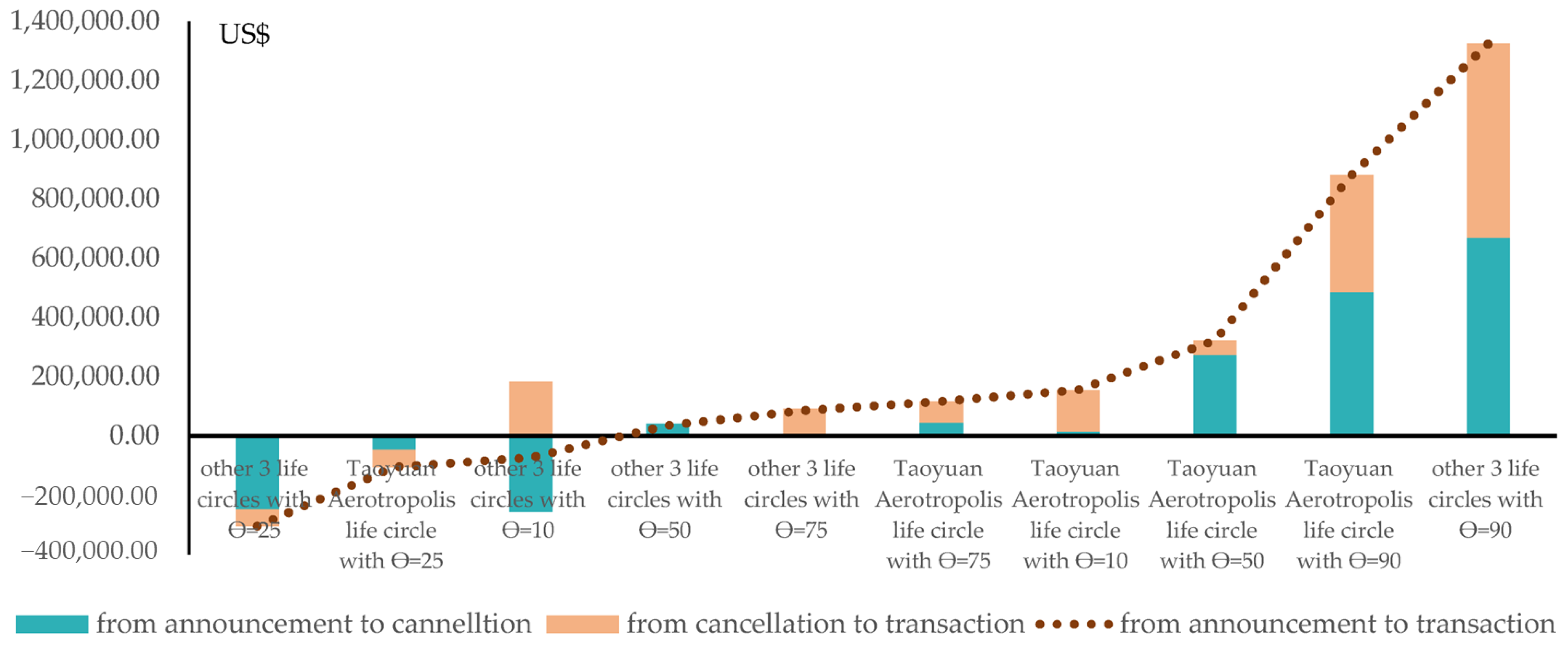
Average months of transacted farmland in Taoyuan Aerotropolis life circle from announcing a controlled site to the cancellation of the site (USD/month)279.64−850.015014.12838.258874.13
Average months of transacted farmland in other 3 life circles from announcing a controlled site to the cancellation of the site (USD/month)−3629.92−3512.78597.13−84.829454.52
Average months of transacted farmland in Taoyuan Aerotropolis life circle from the cancellation of a site to the transaction (USD/month)5616.74−2342.641945.822859.3415,892.71
Average months of transacted farmland in the other 3 life circles from the cancellation of a site to the transaction (USD/month)3985.74−1222.61−154.112001.6814,250.66
The average duration of the nearest announced controlled site prior to the date of a specific piece of transacted farmland (USD/month)1114.952155.12−2626.80−376.98−9903.79
The average duration of the nearest cancelled controlled site prior to the date of a specific piece of transacted farmland (USD/month)−6116.48−540.772156.09−2112.65−5093.18
The distance between the transacted farmland and the nearest controlled farmland (USD/meter)3061.301637.38463.85542.7863.03
The distance between the transacted farmland and the nearest cancelled contaminated controlled farmland (USD/meter)−3275.15−2427.29−950.97−904.86−203.05
The price of a construction site in Taoyuan Aerotropolis life circle (USD/meter)62.1072.435.600.30−1.90
The price of a construction site in the other 3 life circles (USD/meter)58.1961.579.461.93−1.47
The distance between transacted farmland in Taoyuan Aerotropolis life circle and its nearest main traffic artery (USD/1000 m)2,854,043.262,904,022.75821,320.68110,342.66−198,448.04
The distance between transacted farmland in the other 3 life circles and its nearest main traffic artery (USD/1000 m)−1,452,537.24−1,366,066.75−370,619.40−107,227.676995.91
Table 6. Total benefit contributed by each factor for the cancellation of contaminated farmland transaction price.
Impact Factor of Total Benefit aQuantile b
θ = 10 θ = 25 θ = 50 θ = 75 θ = 90
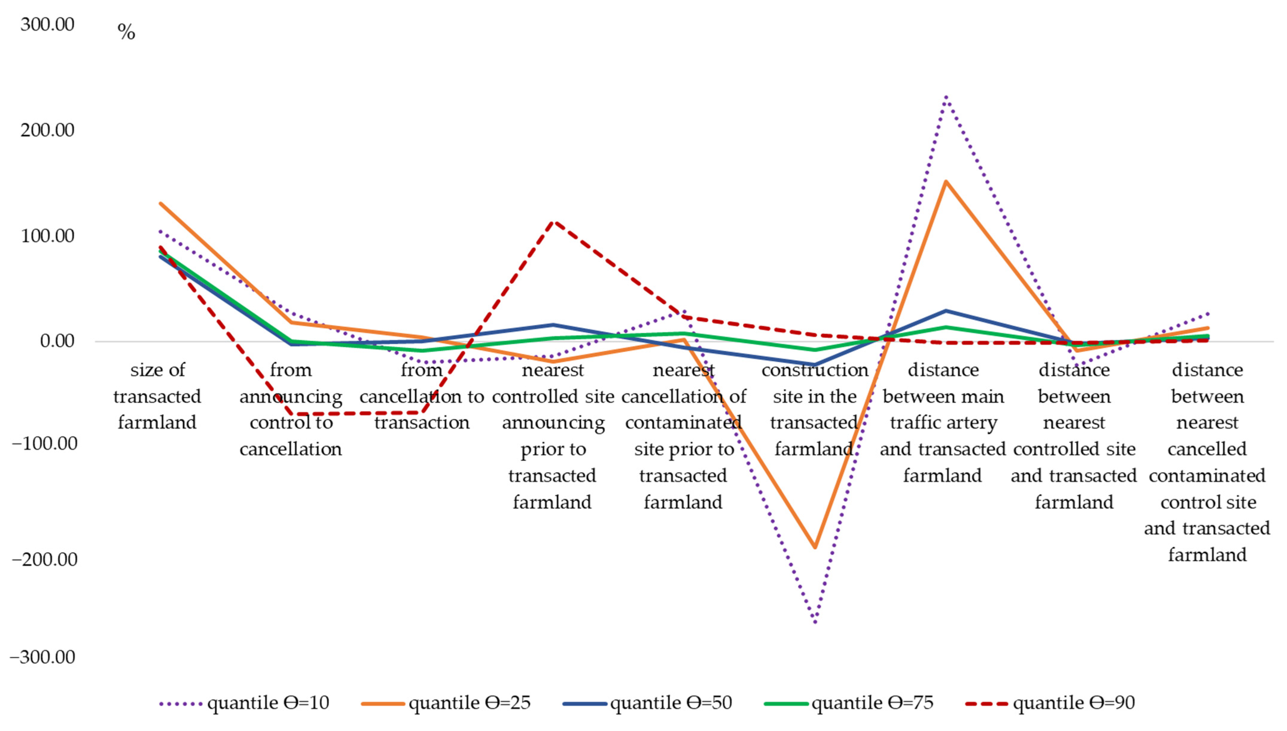
Benefit of the average size of transacted farmland in the Taoyuan Aerotropolis life circle (1300 m2)5,096,977.03
(45.03%)
8,157,459.27
(55.02%)
8,142,007.46
(85.58%)
6,854,796.18
(97.80%)
7,170,866.32
(105.20%)
Benefit of the average size of transacted farmland in the other 3 life circles (970 m2)−976,856.64
(104.31%)
−1,766,619.77
(131.24%)
−1,501,390.43
(80.67%)
−990,983.45
(85.93%)
−882,087.94
(89.81%)
Benefit of the average months of transacted farmland in Taoyuan from announcing a controlled site to the cancellation of the site (54.68 months)15,291.50
(0.14%)
−46,479.75
(−0.31%)
274,170.65
(2.88%)
45,835.24
(0.65%)
485,238.50
(7.12%)
Benefit of the average months of transacted farmland in the other 3 life circles from announcing a controlled site to the cancellation of the site (70.75 months)−256,818.03
(27.42%)
−248,527.78
(18.46%)
42,246.29
(−2.27%)
−6000.13
(0.52%)
668,906.63
(−68.10%)
Benefit of the average months of transacted farmland in the Taoyuan Aerotropolis life circle from the cancellation of a site to the transaction (24.92 months)139,969.25
(1.24%)
−58,378.59
(−0.39%)
48,488.52
(0.51%)
71,255.64
(1.02%)
396,047.90
(5.81%)
Benefit of the average months of transacted farmland in the other 3 life circles from the cancellation of a site to the transaction (46.03 month)183,462.02
(−19.59%)
−56,278.22
(4.18%)
−7,092.85
(0.38%)
92,138.32
(−7.99%)
655,957.60
(−66.79%)
Benefit of the average duration of the nearest announced controlled site prior to the date of a specific transacted farmland in the Taoyuan Aerotropolis life circle (78.54 months)87,567.89
(0.77%)
169,263.23
(1.14%)
−206,307.66
(−2.17%)
−29,608.06
(−0.42%)
−777,844.66
(−11.41%)
Benefit of the average duration of the nearest announced controlled site prior to the date of a specific transacted farmland in the other 3 life circles (114.19 months)127,314.66
(−13.59%)
246,093.70
(−18.28%)
−299,954.20
(16.12%)
−43,047.83
(3.73%)
−1,130,913.43
(115.14%)
Benefit of the average duration of the nearest cancelled contaminated controlled site prior to the date of a specific transacted farmland in the Taoyuan Aerotropolis life circle (24.55 months)−150,160.31
(−1.33%)
−13,276.19
(−0.09%)
52,931.36
(0.56%)
−51,864.82
(−0.74%)
−125,037.62
(−1.83%)
Benefit of the average duration of the nearest cancelled contaminated controlled site prior to the date of a specific transacted farmland in the other 3 life circles (45.37 months)−277,504.42
(29.63%)
−24,533.80
(1.82%)
97,821.11
(−5.26%)
−95,851.60
(8.31%)
−231,077.01
(23.53%)
Benefit of the distance between a transacted farmland in the Taoyuan Aerotropolis life circle and its nearest controlled site (56.30 m)172,351.63
(1.52%)
92,184.13
(0.62%)
26,113.98
(0.27%)
30,560.10
(0.44%)
3549.70
(0.05%)
Benefit of the distance between a transacted farmland in the other 3 life circles and its nearest controlled site (69.00 m) 211,228.16
(−22.56%)
112,978.47
(−8.39%)
32,006.15
(−1.72%)
37,453.38
(−3.25%)
4347.97
(−0.44%)
Benefit of the distance between a transacted farmland in the Taoyuan Aerotropolis life circle and its nearest cancelled contaminated controlled site (65.14 m)−213,341.62
(−1.88%)
−158,113.59
(−1.07%)
−61,947.92
(−0.65%)
−58,941.31
(−0.84%)
−13,227.12
(−0.19%)
Benefit of the distance between a transacted farmland in the other 3 life circles and its nearest cancelled contaminated controlled site (75.61 m)−247,634.63
(26.44%)
−183,527.45
(13.63%)
−71,903.42
(3.86%)
−68,415.89
(5.93%)
−15,353.66
(1.56%)
Benefit of the price of a construction site in the Taoyuan Aerotropolis life circle (US$1431.22)2,716,452.92
(24.00%)
3,168,716.87
(21.37%)
245,167.83
(2.58%)
13,168.23
(0.19%)
−83,154.49
(−1.22%)
Benefit of the price of a construction site in the other 3 life circles (US$1393.94)2,479,117.32
(−264.72%)
2,623,388.73
(−194.88%)
403,127.66
(−21.66%)
82,241.71
(−7.13%)
−62,448.47
(6.36%)
Benefit of the distance between a transacted farmland in the Taoyuan Aerotropolis life circle and its nearest main traffic artery (1210 m)3,453,392.66
(30.51%)
3,513,868.35
(23.70%)
993,797.03
(10.45%)
133,514.36
(1.90%)
−240,123.01
(−3.52%)
Benefit of the distance between a transacted farmland in the other 3 life circles and its nearest main traffic artery (1500 m)−2,178,806.52
(232.65%)
−2,049,100.31
(152.22%)
−555,928.16
(29.87%)
−160,842.11
(13.95%)
10,495.32
(−1.07%)
Total benefit of the Taoyuan Aerotropolis life circle
(total %)
Total benefit of the other 3 life circles
(total %)
11,318,500.95
(100.00%)
−936,498.08
(100.00%)
14,825,243.73
(100.00%)
−1,346,126.43
(100.00%)
9,514,421.25
(100.00%)
−1,861,067.85
(100.00%)
7,008,715.56
(100.00%)
−1,153,307.60
(100.00%)
6,816,315.52
(100.00%)
−982,172.99
(100.00%)
Notes: a: The magnitudes in parentheses under the column of the impact factor are the average of each factor in the related transaction life circle. b: The numbers in the parentheses under each quantile are the percentages of each factor provided to the total benefit of different life circles.
Disclaimer/Publisher’s Note: The statements, opinions and data contained in all publications are solely those of the individual author(s) and contributor(s) and not of MDPI and/or the editor(s). MDPI and/or the editor(s) disclaim responsibility for any injury to people or property resulting from any ideas, methods, instructions or products referred to in the content.

