Article

A Framework to Identify Priority Areas for Restoration: Integrating Human Demand and Ecosystem Services in Dongting Lake Eco-Economic Zone, China

1
Hengyang Key Laboratory of Ecological Regional-Urban Planning and Management, University of South China, Hengyang 421001, China
2
Songlin College of Architecture and Design Art, University of South China, Hengyang 421001, China
*
Author to whom correspondence should be addressed.
Land 2023, 12(5), 965; https://doi.org/10.3390/land12050965
Submission received: 14 March 2023 / Revised: 20 April 2023 / Accepted: 24 April 2023 / Published: 26 April 2023

Abstract

:
The identification of priority restoration areas (PRAs) for ecosystems is a critical step in establishing restoration programs. Because the majority of existing studies focused on improving the ecosystem supply, the PRAs selected are likely to be remote from human demand, and the restoration benefits will not flow to humans. To fill this gap, we constructed an improved framework integrating the ecological restoration projects’ cost and benefits as indicators for choosing PRAs. Then, we identified PRAs for each ecosystem service (ES) with Marxan, and ranked the restoration priority grades according to the superimposed value of PRAs for each ES. Finally, we adjusted the restoration priority grades based on human demand and the concentration of those areas, and chose PRAs with a high ES supply and demand. This framework was applied to the Dongting Lake Eco-Economic Zone, one of China’s most significant ecological restoration project sites. The results indicated that the areas with “high”-, “sub-high”-, and “low”-grade PRAs, based only on the increase in the ES supply, were equal to 82, 410, and 1696 km2, respectively. After considering human demand, the PRAs moved continuously towards places with a high human demand; high-priority areas grew to reach 144 km2, while low-priority areas decreased to 1498 km2. The upgrade of the proposed framework for the identification of PRAs can contribute to increasing human well-being, while also serving as a support tool for environmental restoration management.

1. Introduction

Ecological issues such as biodiversity loss and land degradation have recently emerged under the double pressure of global climate change and human activities, seriously threatening human well-being and sustainable development [1,2,3]. China is one of the countries that have been suffering from serious ecological degradation. In order to ensure the sustainable supply of ecosystem services (ESs), the restoration of ecologically degraded areas has become an important objective of ecosystem management [4,5,6]. Nevertheless, inadequate financing constrains the large-scale implementation of ecological restoration [7,8]. For the sake of improving the efficiency of restoration and achieving the related goals as soon as possible, it is particularly important to scientifically delineate priority restoration areas (PRAs) [9,10].
Potential restoration areas (PoRAs) need to be identified before prioritizing restoration areas. To this purpose, current research mainly applied the criteria of site suitability [11,12], ecosystem pattern [13,14], and quality [15,16,17]. Suitability-based studies typically apply land-use rationalization methods, such as converting space that is unsuitable for cropland to other land-use types (e.g., forests or grassland) [18]. Ecosystem-pattern-based studies prioritize the preservation of an ecosystem’s natural pattern, such as the restoration of forest that has been converted to grassland [19]. Finally, quality-based studies, which are the most commonly performed, include both narrow and broad spatial scales. At narrow scales, integrated indicators (e.g., tree attributes, plant species diversity, and forest biological productivity) are typically used, including detailed information on the forest ecosystem structure [20], biodiversity composition [21], and function [22,23]. At broad spatial scales, ecological restoration aggregation indicators are frequently gathered through field surveys or long-term monitoring [24,25]; as such, it is difficult to adopt them, due to the time-consuming data-collection process. Therefore, some scientists developed complicated ecological models to estimate the native forest community biomass at the pixel scale as a quality-assessment standard for broad spatial scales [26,27]. Although these approaches improve the accuracy of the ecosystem quality assessment, they need a vast volume of data.
The primary aim of ecological restoration is to enhance the ES supply [22]. Therefore, several researchers, from the perspective of the ES supply, identified areas with a low ES supply but are critical for the development of ecological security patterns as PRAs [22,28,29]. Although this approach improves the structural integrity of the ecosystem and ensures ecological benefits, it fails to account for human demand. In fact, the mismatch between the ESs’ supply and demand usually occurs when ESs are provided in places where there is no human demand, or when ESs are not insufficient for human demand [30]. Therefore, a focus solely on the ESs’ supply without considering human demand may not provide direct restoration benefits to human society, which will result in a loss of ESs. [31]. Furthermore, as ESs are a vital source of livelihoods for those in impoverished areas, ecological restoration neglecting human demand will destroy human well-being [32,33]. Hence, works of research integrating ESs and human demand into ecological restoration have gained much attention, such as establishing key protection areas in regions with a low ES supply and high human demand [34], considering the ESs’ supply–demand balance to optimize the ecosystem configuration [35], integrating the ESs’ supply–demand with the relevance of ecosystem protection and restoration to support regional sustainable management [36], etc. These studies have enriched the practice of ecological restoration by applying the exploration of the relationship between ESs and human demand to ecological restoration and protection. However, the cost-effectiveness of restoration has not been emphasized in these works of research. As restoration projects have spread over an increasing number of regions and countries, a planning solution that balances the restoration costs and benefits must be urgently developed. In order to solve these problems, several optimization strategies have been proposed and are rapidly becoming a hot topic of current research; these include the use of linear-programming techniques to optimize the biodiversity or ES in protection areas [37], and the use of heuristic algorithms to identify unknown optimal conservation solutions for protected areas, which, however, faces the problem where large data volumes are required [38]. Marxan, as a system-protection-planning model, can minimize computing effort by applying it to the identification of PRAs, employing a simulated annealing approach to obtain the ideal solution after numerous iterations based on the weighting of multiple indicators [39,40].
To address these issues, we developed an optimized framework to prioritize ecological restoration areas. According to this framework, PoRAs were defined as the area where the ESs’ potential supply declines above the mean value. Moreover, Marxan was used to define low-cost, high-supply areas as PRAs for individual ESs. PRAs were then classified based on the overlap of those for the individual ESs, and revised based on human demand and aggregation. This framework was applied to the case-study area of the Dongting Lake Eco-Economic Zone, which is one of China’s major ecological restoration project sites and an important ecological barrier in Hunan Province. The objectives of this study were to develop an optimized ES-based framework to identify PRAs, and include the intensity of human demand for ESs as an indicator to determine the grade of the PRAs, in order to provide a theoretical basis for ecosystem restoration practices.

2. Materials and Methods
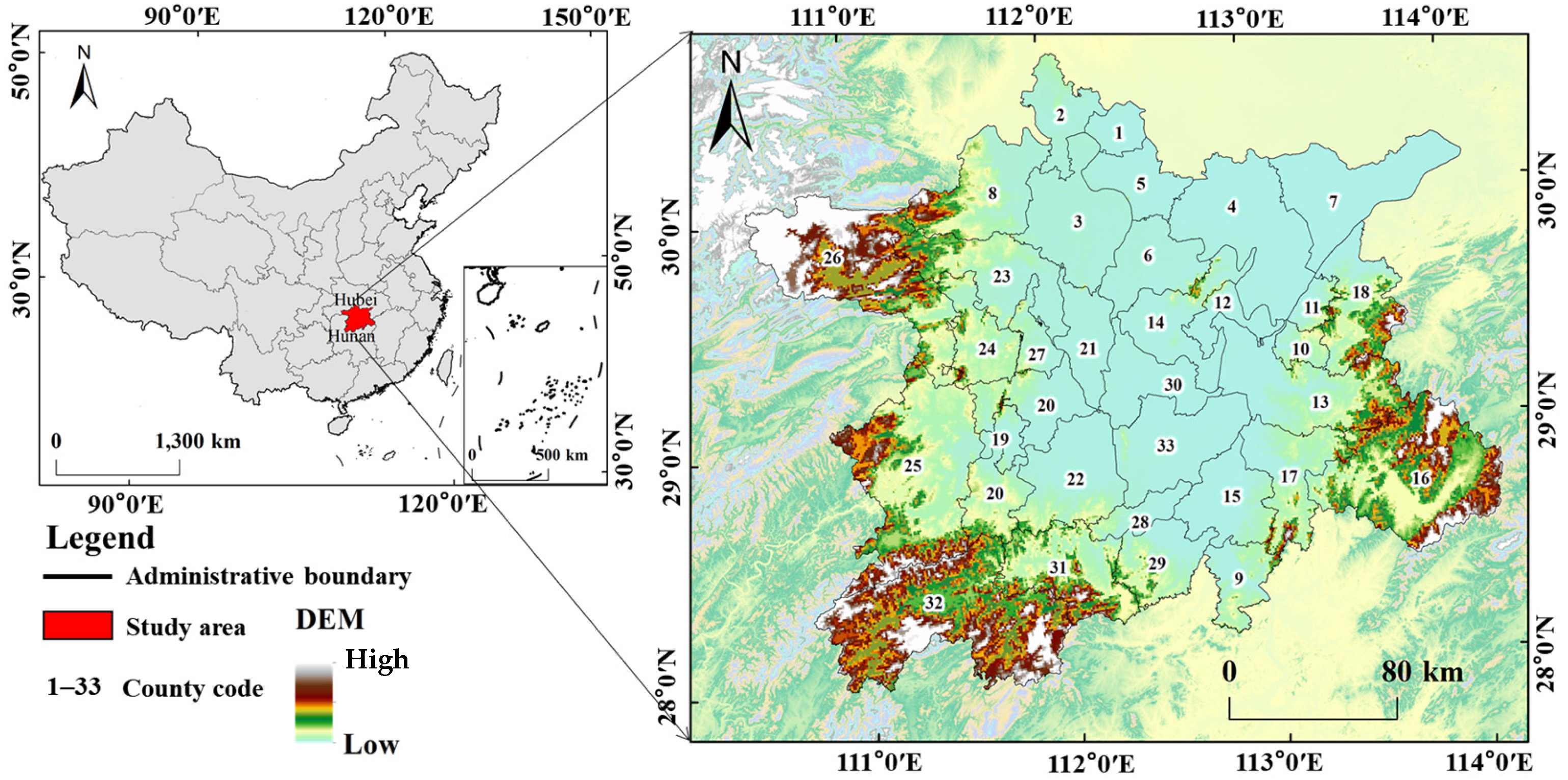
2.1. The Study Area

The Dongting Lake Eco-Economic Zone (27°58′–31°37′ N, 110°21′–114°09′ E) includes 4 cities and 1 district. It is located in the north of Hunan Province, and has a total area of 61,000 km2 [41] (Figure 1). This area is characterized by a subtropical monsoon climate, abundant annual precipitations, and a well-developed water system; as such, it is a fundamental water storage ecological zone in the middle and lower reaches of the Yangtze River, as well as an important grain- and cotton-producing area [42]. The diverse topography and favorable climate have resulted in an abundance of biological resources, concentrated at the node where the conjugate and divergent Yangtze River systems coexist, thereby entailing a high ecosystem sensitivity and vulnerability. In recent years, climate change and intense human activities have damaged the Zone’s ecosystem, resulting in a series of ecological issues such as environmental pollution, biodiversity reduction, and the shrinking of lakes [43].

2.2. Datasets

The data used in this study were obtained from the sources given below, and the access dates for all data are 15 April 2021.
  • The land-use maps for 2000, 2005, 2010, 2015, and 2020 (30 m resolution) were obtained from the Resource Environment and Science Data Center of the Chinese Academy of Sciences (https://www.resdc.cn/, accessed on 13 March 2023). Based on the characteristics of the ecosystem composition of the study area, land-use types were reclassified into six categories: cropland, forest, grassland, water bodies, artificial land, and unused land.
  • Average annual rainfall, evaporation, and temperature data were downloaded from the China Meteorological Data Service Center (http://data.cma.cn/, accessed on 13 March 2023).
  • The net output productivity (NPP, 100 m resolution) data were retrieved from the website of National Aeronautics and Space Administration (NASA) (https://www.nasa.gov/, accessed on 13 March 2023).
  • The Digital Elevation Model (DEM, 90 m resolution) was taken from the Geo-spatial Data Cloud (https://www.gscloud.cn/, accessed on 13 March 2023).
  • Soil classification and data on associated soil attributes were obtained from the 1:1 million digital soil map of China and the Second National Soil Survey of China (http://www.ncdc.ac.cn/portal/, accessed on 13 March 2023).
  • Socioeconomic, population density (1000 m resolution), and road, river, and settlement data were obtained from the Resource and Environment Science and Data Center (https://www.resdc.cn/, accessed on 13 March 2023).
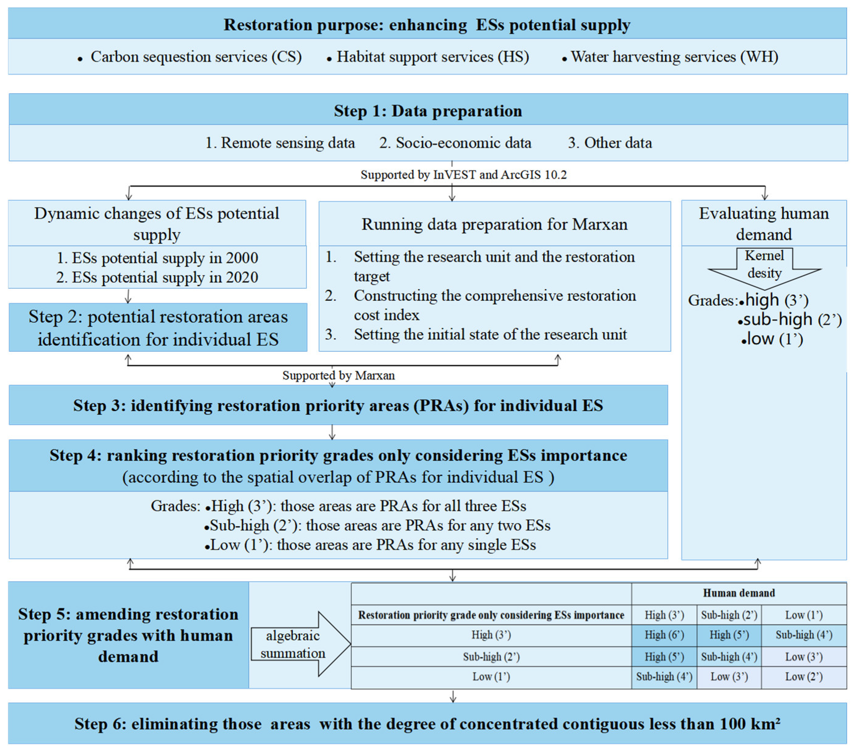
All raster data were modified to a spatial resolution of 100 m using the ArcGIS resampling tool.

2.3. Methods

We selected the year 2000 as the starting point for our study, considering the significant milestone achieved by China’s economic growth and rapid urbanization, as well as the implementation of ecological policies during that time. In addition, we employed a research timeframe of 20 years, spanning from 2000 to 2020. Figure 2 illustrates the methodological framework employed in this study for the identification of PRAs and ranking of restoration priority grades, which is comprehensively articulated into six steps. The initial step entailed leveraging pre-compiled foundational data to calculate the potential supply and demand of ESs. Afterwards, PoRAs were determined based on the dynamic changes of ES potential supply from 2000 to 2020. Subsequently, it was essential to collate the requisite data for Marxan to establish the foundation for the identification of PRAs of individual ES. A critical component of this step was the development of a comprehensive restoration cost index. In addition, Marxan was used to facilitate the identification of the PRAs for each ES that incorporated both restoration costs and benefits among the PoRAs. In the fourth step, the restoration priority grade, considering only ESs’ importance, was ranked based on the spatial overlap analysis of the three PRAs maps. The basic settings were as follows: planning units with PRAs for all three ESs were assigned the highest restoration priority grade, while those with PRAs for any two ESs were assigned a sub-high priority grade, and those with PRAs for any single ES conferred the lowest priority grade. The fifth step was to revise the restoration priority grades using human demand. Finally, the areas with an aggregation degree of less than 100 km2 were eliminated from the PRAs.

2.3.1. Accounting for Potential Supply of ES

Comprehensively considering the Chinese government’s carbon management goals and the distinct function of the study area within the ‘National Ecological Function Zoning’, as well as the special environment demand of the research area’s industrial characteristics, we ultimately chose three representative ESs in demand, namely, carbon sequestration (CS), habitat support (HS), and water harvesting (WH), for the purpose of research.
(1)
Carbon sequestration (CS)
CS is the process through which atmospheric CO2 is fixed in plants and soil [44]. The amount of CS was calculated using the CS module in the InVEST model [45], as follows:
Q c = i = 1 n Q i × S i × F N E P × 10 9
where Qc indicates the total CS of the ecosystem (t·yr−1); Qi indicates the amount of carbon sequestration of land-use type i (Mg·yr−1), including the organic carbon density of above-ground, below-ground, soil, and dead organic matter, respectively (Mg·hm−2·yr−1); Si indicates that area of land-use type i (hm2); and FNEP represents the spatial correction factor of net ecosystem productivity (NEP), which was obtained using the affiliated fuzzy method based on the mean value for the study area. NEP was obtained by NPP conversion.
(2)
Habitat support (HS)
Habitats are the natural environment that offers living space for a certain species or population within a specific region; as such, they are frequently used as an indication of biodiversity [46]. The Habitat Quality module of the InVEST model was utilized to quantify HS [47], as follows:
S Q i j = H i × [ 1 D i j z / ( D i j z + K z ) ]
where SQij is the habitat quality index in cell i of land-use type j; Dij is the habitat degradation index in cell i of land-use type j; z and k are constants; and Hj is the habitat suitability of landscape j. All parameters are dimensionless.
(3)
Water harvesting (WH)
Following the water balance equation [48], WH was calculated as follows:
Q w = i = 1 j ( P i R i E T i ) × A i × 10 3
where QW is the amount of WH (m3·yr−1); Pi represents precipitation (mm); Ri denotes rapid runoff (mm); ETi indicates evapotranspiration; and Ai represents the area of ecosystem i (m2).

2.3.2. Accounting for the Importance of ES Demand

Relative inequalities in socioeconomic development and natural resource availability within a certain zone result in disparities in ES demand. The concept of ‘point of interest’ (POI) refers to the spatial distribution of geographic entities in a city that are closely linked to human activities, including food and beverage services, medical education, and residential and recreational places, reflecting the density of population and socioeconomic activities. In general, the spatial distance between an ecological site and a POI impacts the level of demand for the ecological site. The POI data were treated in ArcGIS 10.2 using the kernel density analysis tool, with a search radius of 30 km. The generated POI kernel density raster map was divided into three classes—high, medium, and low—utilizing geometric intervals to ensure that the ecological demand is positively correlated with the kernel density classes, as follows:
f x = i = 1 n 1 D 2 × k × ( x c i D )
where f(x) is the image element x’s kernel density calculation function; k is the spatial weight function; D is the distance decay queue; and ci is the raster x distance in the search decay range of all POIs. All parameters are dimensionless.

2.3.3. Identifying PoRAs

The potential supply of CS, HS, and WH was standardized using Equation (5). By comparing the potential supply in 2000 with the current situation, the areas where the supply decreased more than the average value were defined as PoRAs for each ES, as follows:
E S x = E S s t E S m i n E S m a x E S m i n
where ESx denotes the standardized value of ESs’ potential supply; ESst represents the current value of ESs’ potential supply; and ESmin and ESmax indicate the minimum and maximum values of ESs’ potential supply.

2.3.4. Marxan

Marxan, a systematic-protection-planning tool, uses simulated annealing methods to provide the most effective protection within specific protection cost restrictions [40]. The basic functions of the model operations are as follows:
S c = c o s t + b o u n d a r y + p e n a l t y
where Sc is the total cost of protection; cost represents the combined cost of the selected planning unit; boundary indicates the sum of the boundary lengths of the selected planning units, whose value represents the strength of connectivity between planning units; and penalty indicates the penalty assigned to the planning system for not effectively representing conservation features. It relies on the idea that if the conservation target is not achieved, then the penalty should be an approximation of the cost of raising the conservation feature up to its target representation level.
Before running the model, the study area was first divided into a certain number of planning units. The commonly used planning units were divided into 3 types: grid cells, hexagonal, and catchment cells. Each planning unit contained a specific area of the protected object and had a specific cost of protection. Then, four initial states were assigned to the planning units based on their attributes (Table 1).

2.3.5. Identifying PRAs with Marxan

(1)
Setting the research unit and the restoration target
The study area was divided into 61,741 cells of 1000 × 1000 m as the fundamental restoration cells using the “Create Fishing Grid” tool of ArcGIS 10.2. Following the Aichi Biodiversity Convention, which set the target of restoration of 15% of a damaged habitat to significantly improve biodiversity [49], the restoration target was chosen as equal to 15% of the PoRAs.
(2)
Constructing the comprehensive restoration cost index
As stated in the “Announcement on the Implementation Plan for the Comprehensive Management Plan of Dongting Lake Water Environment in Hunan Province (2018–2025)”, the cost of the Dongting Lake water ecological restoration project was 5.4 million yuan/hm2. In parallel, in accordance with the “Implementation Standards for Restoration of Vegetation and Forestry Production Conditions in Hunan Province (trial version)”, the investments necessary to restore forest and grassland vegetation were 2 and 3 million yuan/hm2, respectively. Hunan Province is mainly characterized by paddy fields as the main type of cultivated land; according to the available data, the approximate cost for the restoration of paddy fields is 1.5 million yuan/hm2. As the cost of ecological restoration is influenced by the ecological quality of the restored area, as well as by the difficulty of the restoration project, the cost data were spatially adjusted using the slope, the distance-to-road/settlement/river, and the GDP/population density [50], as follows. Initially, these indicators were reassigned based on the ecological meaning of the aforementioned indicators (Table 2); subsequently, the reassigned indicator values were utilized to modify the ecological restoration project costs of each ecosystem. However, in some parcels of land the costs and benefits of restoration were not comparable; therefore, focusing solely on low prices could result in poor benefits for the PRAs. To address this issue, we quantified restoration benefits as the largest difference on a long-term pixel scale, and integrated the cost of ecological restoration project with the reassigned restoration benefits to calculate the ecological restoration cost. To avoid the magnitude effect, we equalized the ecological restoration project costs and restoration benefits. The formulae employed are as follows:
C i = P i × j = 1 n L j
η i = C i + B i
where Ci indicates the amended cost of the ecological restoration project for planning unit i; Pi represents the cost of the ecological restoration project for planning unit i, which is determined by the land-use type of planning unit i; Li indicates the revised indicators after reassignment; n is the number of restoration cost indicators; Bi indicates the restoration benefits; and i is the comprehensive cost index. To avoid a negative “cost” parameter in Marxan, we reassigned the restoration benefits in order of magnitude, and the ecological restoration cost is obtained by adding the restoration project cost to the reassigned restoration benefits.
(3)
Setting the initial state of the research unit
According to the description of different initial states for planning units in Table 1, we set the initial state of research units as follows: (i) As the surface of artificial land is irreversible, we assigned the initial status for the planning units with the artificial land as equal to 3, to ensure that those units would definitely not appear in the final plan. (ii) We established a 15% restoration target in this research, which indicates that a portion of the PoRAs will be identified as PRAs. Consequently, the initial state of the planning units for PoRAs was set to 1. (iii) The other remaining units were set to 0.

2.3.6. Classification of the Priority Grade, Only Considering Ecological Importance

We overlapped the spatial distribution maps of PRAs for CS, HS, and WH to obtain the ecological restoration priority grade. By default, Marxan assigned value of 1 to the PRAs, and a value of 0 to other planning units. Then, we used the Raster calculator tool of ArcGIS 10.2 to integrate the spatial distribution maps of the PRAs for three ESs. According to the results, the planning units with a value of 3 had the highest restoration priority grade, followed by the planning units with a value of 2, while those with a value of 1 had the lowest restoration priority grade.

2.3.7. Modifying the Restoration Priority Grades, Considering Human Demand and Aggregation Degree
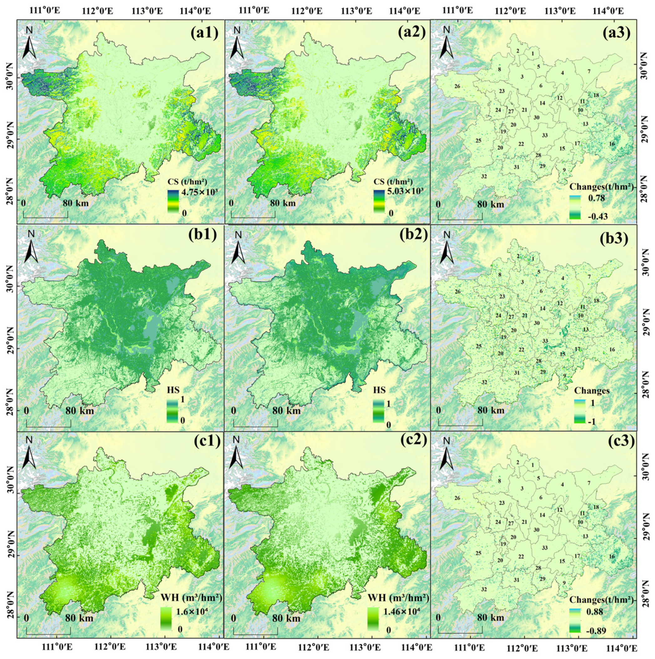
Based on the importance of ES, both PRAs and the importance of ecological demand were assigned a value from 3 to 1 from highest to lowest. According to the algebraic summation, the ecological restoration priority grade was modified using the importance of ecological demand (Table 3).
Long-term ecological restoration activities have demonstrated the need for concentrated and large-scale treatment to produce comprehensive benefits. Based on the characteristics of the study area, we eliminated from the PRAs those image cells with an aggregated area of less than 100 km2. Then, with the support of the Grid module in ArcGIS 10.2, the “docell” command was used to conditionally select the PRA layers corrected for demand importance with the aggregation layer, resulting in PRAs combining aggregation, demand importance, and ecological importance.

3. Results

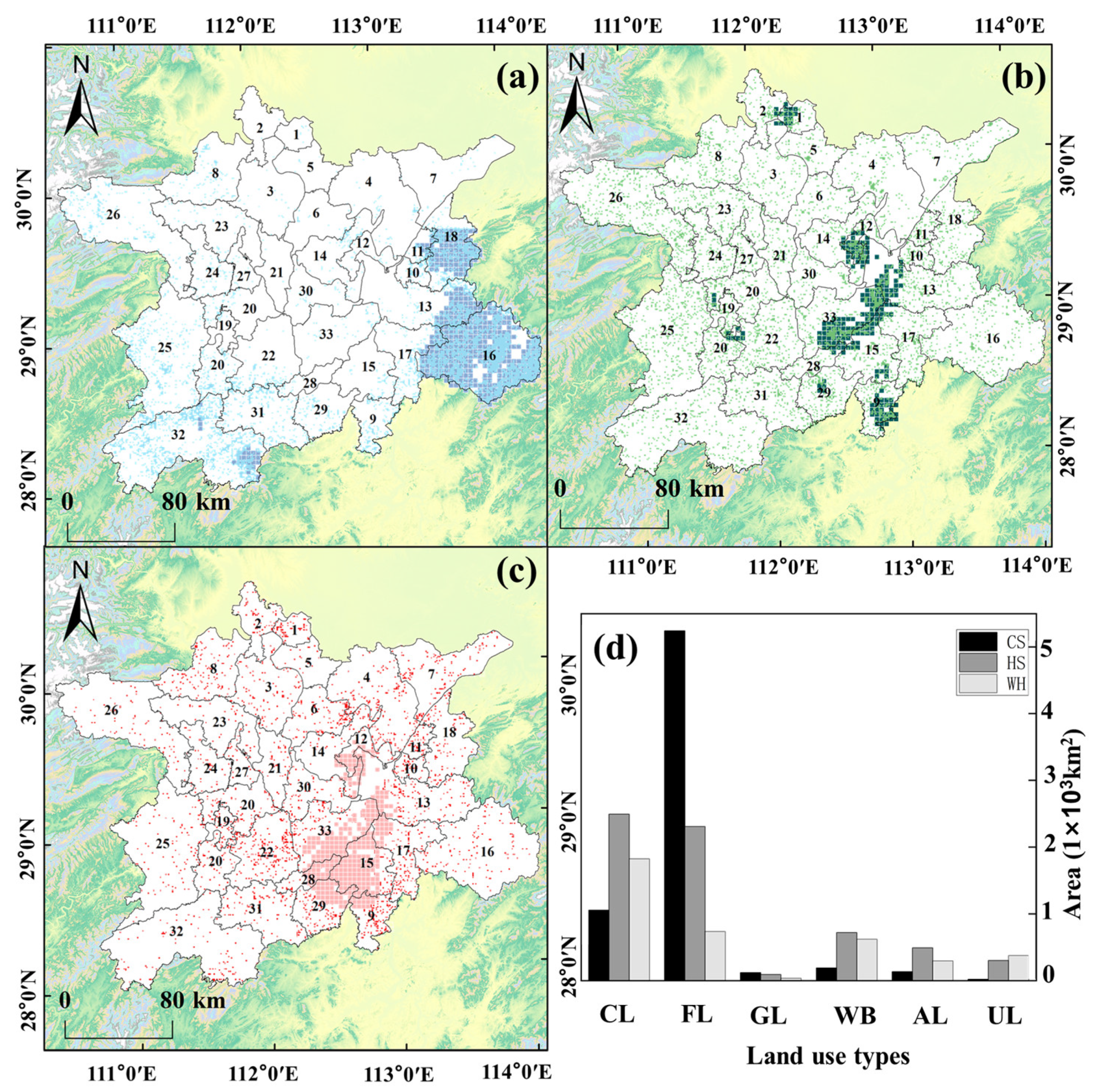
3.1. Potential Supply of ES

The ecological function spatial pattern reflects ES spatial heterogeneity. In both 2000 and 2020, the spatial distribution of CS increased from the center to the periphery (Figure 3(a1,a2)). This is mainly attributed to the fact that the level of CS is primarily dependent on the land-use types. The area with a high CS value was located in the northwestern portion of the study area, characterized by forest with a high carbon density and CS capability. The central area, which includes cropland and water bodies, had a low value of CS. The spatial distribution of HS followed those sites characterized by a perfect ecological background and the absence of strong human disturbance. Accordingly, HS was higher in the eastern and western parts of the study area and Dongting Lake, where several national nature reserves are located, guaranteeing high levels of biodiversity. In contrast, those areas with low HS were mainly located in the cropland-dominated central area and other artificial land area (Figure 3(b1,b2)). Finally, WH depends on the water storage capacity of vegetation. WH was higher in the eastern and southwestern parts of the study area, characterized by high annual precipitation (Figure 3(c1,c2)), abundant vegetation, and strong water storage capacity. Areas with low WH were mainly found in the central part of the study area, characterized by low precipitation, mono-vegetation, and rapid evaporation.
In terms of the evolution of the spatial pattern from 2000 to 2020, CS recorded a small increase, with the area of the increasing and unaltered parts being 27.3% and 58.1% of the study area, respectively, while the part where CS decreased covered 14.6% of the study area, primarily located in County 16 and County 18 (Figure 3(c1)). In parallel, HS showed a significant decline. In more detail, the area of this decline reached 79.2% of the total area, and was primarily located in areas other than Dongting Lake and Hong Lake (Figure 3(c2)). This is attributable to the growing human disturbance, which has caused habitat stress and the deterioration in habitat quality. The areas where HS increased and remained unchanged were equal to 11.7% and 9.1% of the total area, respectively. Finally, WH also marked a reduction, having decreased in 36.3% of the study area. The counties surrounding Dongting Lake, as well as Counties 15, 13, and 12, saw the greatest declines (Figure 3(c3)), owing to the transfer of water to unutilized land. The areas where WH increased and remained unchanged were 46.3% and 17.4% of the total area, respectively, with Counties 4 and 7 as the areas where the greatest increase occurred.

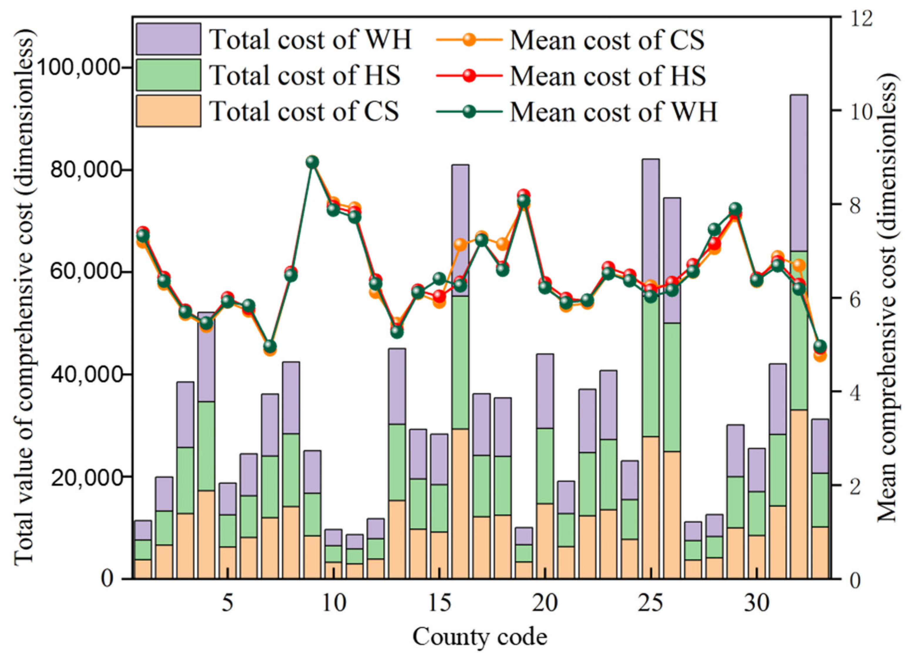
3.2. Comprehensive Cost Index (η)

Ecological restoration costs were ranked as follows: CS (6.29) > HS (6.22) > WH (6.17), indicating that CS had a higher restoration cost and lower benefits, and vice versa for WH (Figure 4). Overall, the majority of counties had minimal differences in the mean value of η for the three ESs, whereas large differences in the proportion of artificial land and ecological land in Counties 15, 16, 18, and 32 resulted in wide variations in the mean value of η for the three ESs. Specifically, at the county scale, those counties η with the smallest county area, such as Counties 1, 10, 11, 12, 19, 27, and 28, had a lower, while the high degree of human disturbance and economic growth in these counties lead to a high mean value of η.

3.3. Potential Restoration Areas

Those areas where the potential ES supply is severely degraded were considered as PoRAs. According to changes in the potential supply of the three ESs from 2000 to 2020, the area of CS-PoRAs was 6759 km2, equal to 38.8% of the CS degraded area, and mainly located in Counties 16, 18, 32, and 31 (Figure 5a). The HS-PoRAs distributed in a scattered manner covered 6407 km2, accounting for 42.9% of the HS degraded area, and were mainly clustered in the counties surrounding the Dongting Lake, the southern part of County 9, and the western part of County 1 (Figure 5b). The spatial distribution of WH-PoRAs was equally scattered, accounting for 12.1% (3887 km2) of the WH degraded area, and concentrated at the junction of Counties 9, 13, 15, 28, and 29 (Figure 5c). In terms of land-use types, forest was the main land-use type in the CS-PoRAs, with an area of 5242 km2, corresponding to 77.5% of the total area of CS-PoRAs (Figure 5d). Cropland was the main land-use type in the WH-PoRA, covering an area of 1823 km2, equal to 46.9% of the total area of WH-PoRA.

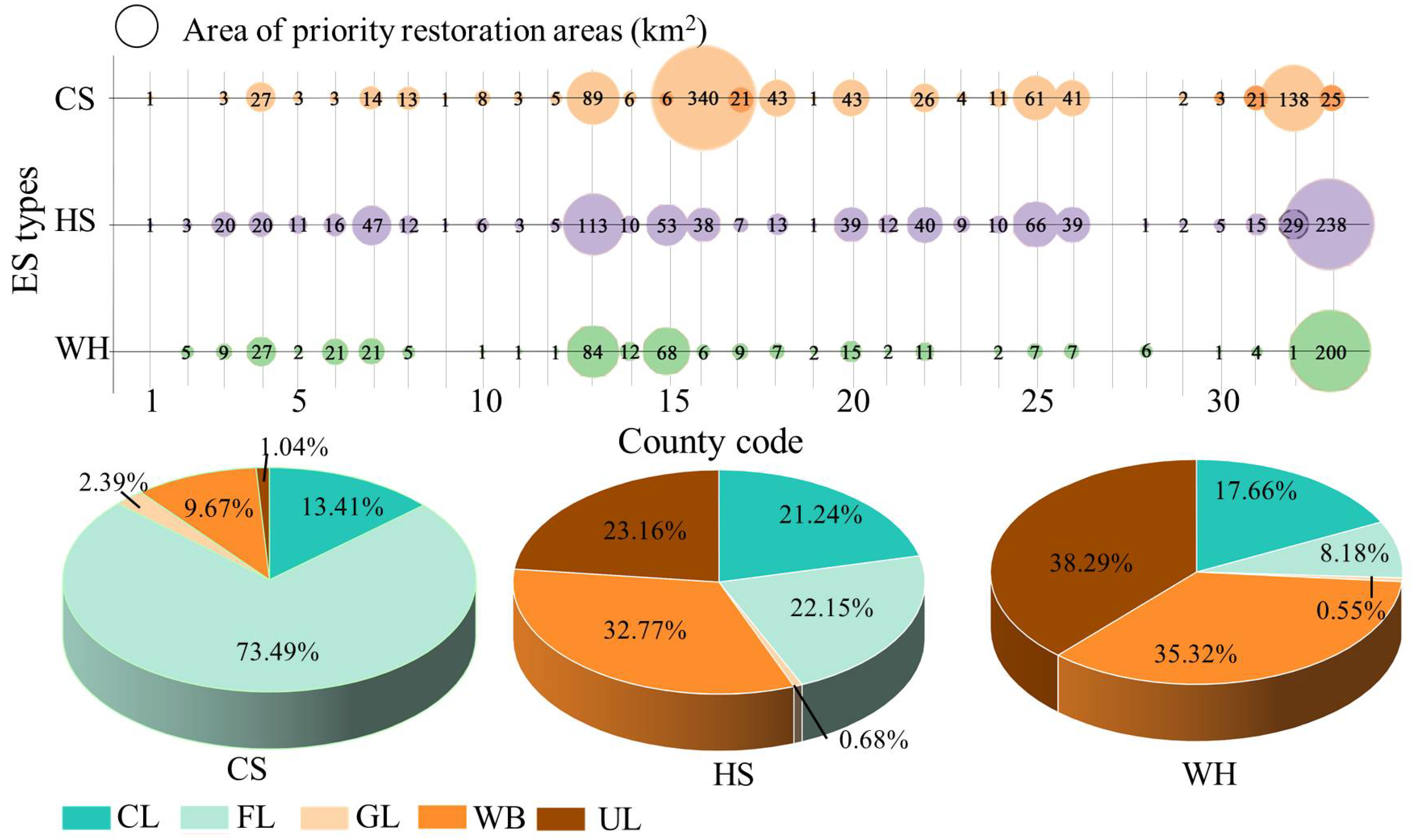
3.4. PRAs for Single ES

Figure 6 shows the spatial distribution of PRAs across counties. The PRAs in CS, HS, and WH occupied 962, 885, and 538 km2 and covered 1.61%, 1.43%, and 0.87% of the entire study area, respectively. The detailed breakdown of the area occupied by each county in the PRAs, displayed in Figure 6, reveals that the CS-PRAs were mainly located in Counties 13, 15, and 12, and the land-use type was mainly forest, accounting for 73.49% of the total area of CS-PRAs. This is mainly due to forest’s high biomass, which entails a great CS after restoration, resulting in significant ecological benefits. HS-PRAs were mainly located in Counties 33, 13, and 25, where they extended for 238 km2, 113 km2, and 66 km2 respectively. Water bodies were the main land-use type for HS-PRAs (32.77%), due to the importance of the Dongting Lake wetlands in conserving biodiversity, particularly for bird species. Other land-use types for HS-PRA were unutilized land, forest, and cropland, with 23.16%, 22.15%, and 21.24% of the total area of HS-PRAs, respectively. WH-PRAs were relatively spatially concentrated in County 33 (200 km2), County 13 (84 km2), and County 15 (68 km2). Unutilized land and water bodies were the main land-use types in WH-PRAs, accounting for 38.29% and 35.32% of the total area of WH-PRAs, respectively, followed by cropland with 17.66%. This is because the unutilized land in these areas was practically converted from water bodies, and restoring these areas back to water bodies can enhance their water retention capacity. It is worth noting that PRAs to promote CS, HS, and WH did not include artificial land, while they included only a small amount of grassland. This is because irreversible changes to the surface of artificial land can result in high restoration costs, while the restoration of grassland produces fewer ecological benefits.

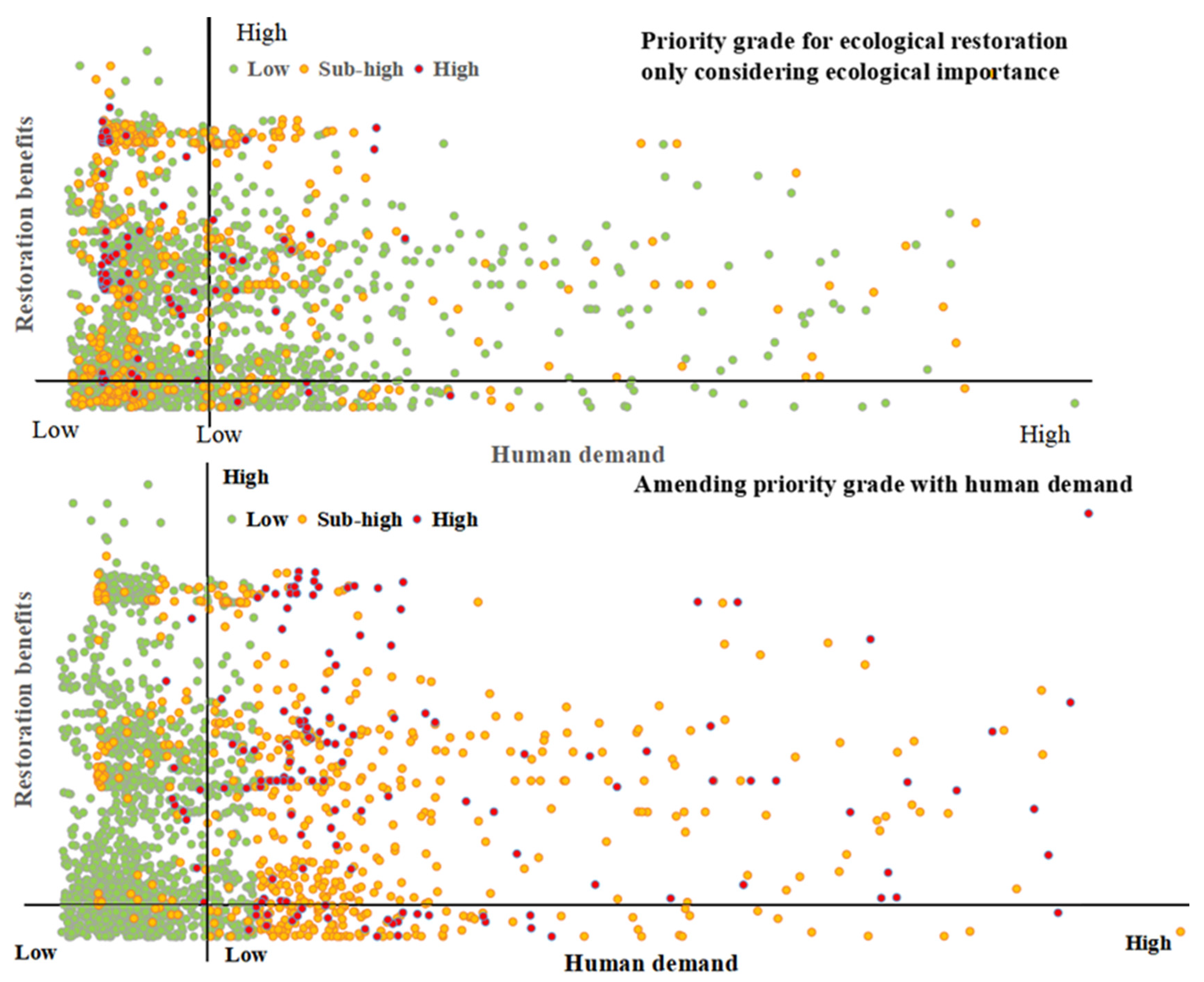
3.5. Restoration Priority Grade Based on ES Importance

The area and spatial distribution of PRAs varied greatly across different priority grades. The PRAs with a “high” ranking were relatively concentrated in the northeastern part of County 33 (Figure 7), with an area of 82 km2 (0.13% of the total study area). The restoration of these areas can promote the synergistic enhancement of CS, HS, and WH. Moreover, these areas were also found to have a low population density, hence resulting in a low restoration cost. Moreover, a large amount of unutilized land degraded from water was included in this area, which could yield significant restoration benefits by converting it into water bodies through ecological measures such as dredging. The area of PRAs with a “sub-high” ranking was 410 km2, the majority of which was devoted to enhancing HS and WH simultaneously (207 km2), and was located primarily in the border areas of County 13, 15, 16, and 33. The PRAs to enhance CS and HS covered 150 km2, scattered in Counties 16, 32, and 3. The area of PRAs to improve CS and WH was only 53 km2 and had a scattered distribution, mostly located in Counties 16, 18, and 33. All other PRAs with a “low” ranking priority covered an area of up to 1696 km2, located mainly in Counties 33, 32, 16, 13, and 12.

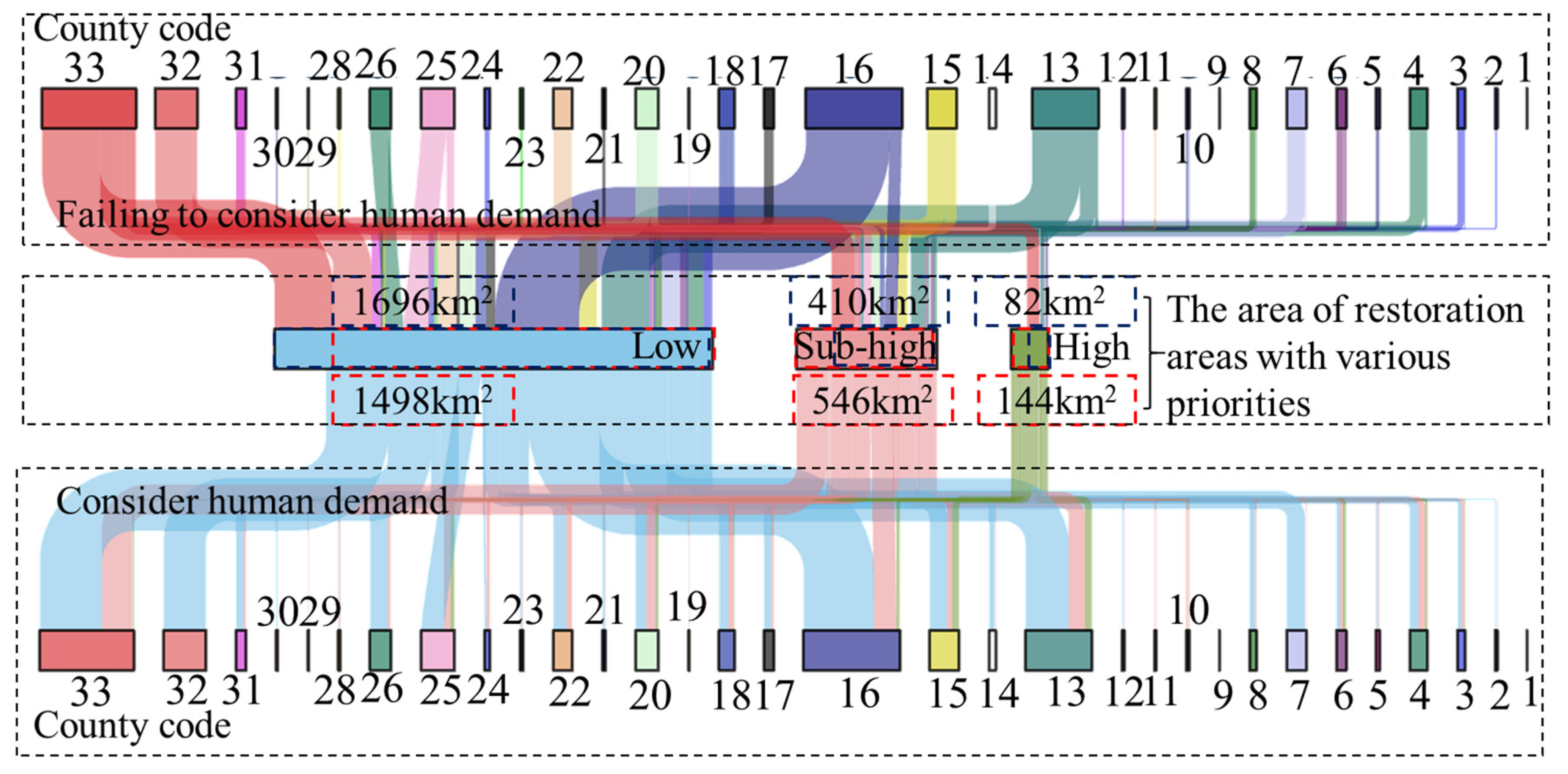
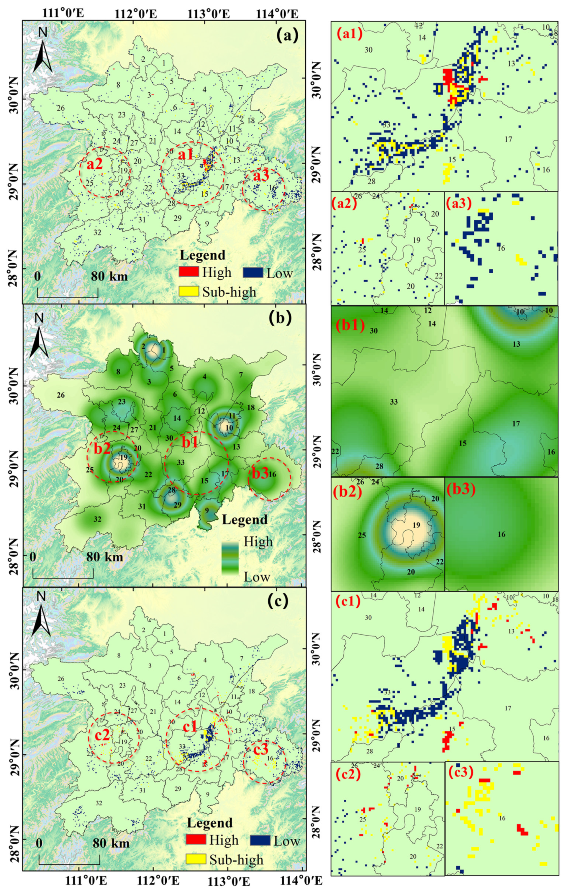
3.6. Revising Priority Restoration Grades Based on Demand Importance and Aggregation Degree

The extent and spatial distribution of the various PRAs, taking into account human demand, were modified as follows: (1) The “high”-grade PRAs increased by 75.61%, reaching 144 km2, and began to shift from County 33 to areas with a “high” human demand and “sub-high” ecological importance, such as Counties 13, 15, and 16 (Figure 8c(c1–c3)). After restoration, these areas allowed the related benefits generated to flow directly to human society (Figure 8b(b1–b3)). In contrast, while the high PRAs in County 33 can offer more restoration benefits, they are relatively poor in terms of socioeconomic development; hence, the initial “high” PRAs were reclassified into “sub-high” PRAs, considering human demand. (2) “Sub-high” PRAs shifted from Counties 15, 33, and the eastern part of County 13, to County 16 and the western part of County 13, covering an area of 546 km2 with an increase of 32.45%. The enlarged portion of sub-high PRAs within County 16 was transformed from low PRAs with significant human demand. (3) “Low” PRAs shrank by 11.36%, with the majority of this reduction occurring in those areas where the original level grade was “high” and “sub-high”.
In order to maximize efficiency, the aggregation areas smaller than 100 km2 were removed from the PRAs, resulting in an improved distribution map of the restoration priority grade. The total area of corrected PRAs shrank by 602 km2, reaching 1586 km2. Specifically, the “high” PRAs decreased by 32 km2 (112 km2), while the “sub-high” and “low” PRAs decreased to 386 km2 (160 km2) and 1088 km2 (410 km2), respectively. Moreover, the geographical distribution of PRAs became more clustered, mainly at the junction of Counties 13, 15, and 33 and within Counties 16, 25, and 32.

4. Discussion

In order to promote the balanced allocation of limited restoration resources among ecologically degraded areas, it is necessary to improve the accuracy of identification for PRAs. Although the current supply-based identification of PRAs can improve the ecological patterns and, thus, increase their potential supply capacity [51], the widespread imbalance between the ES supply and demand undermines the integrity of ES processes and hinders the realization of social benefits from ecosystems [52]. It is well-known that ESs serve as a bridge between the natural and social systems [53]. In this study, we proposed a framework for the identification of PRAs to boost the ESs supply, which integrates the ecological and socioeconomic benefits of restoration and simplifies the identification process using Marxan.
The identification of PoRAs is the foundation for the selection of ecological PRAs [54]. In this respect, our study provided a novel viewpoint on PoRA identification. Several previous studies concentrated on land-use change, considering the land transformed from natural ecosystems to cropland, pastures, and even artificial land as PoRAs [55]. However, with the increase in the intensity of anthropogenic disturbances, a large extension of degraded land did not experience conversion [56], leading to a variety of global difficulties if the land failed to be restored. Because changes in the ES supply may indicate ecosystem conversion and degradation, this study utilized variations in the ES supply over a long period to identify PoRAs. The findings showed that PoRAs for CS, WH, and HS include not only areas converted from forest and water bodies to cropland, but also a large number of degraded forest and water bodies.
Our framework enables the inclusion of ‘low-cost, high-yield supply’ areas in PRAs, thereby boosting resource allocation efficiency and increasing the feasibility of restoration projects in the case of limited restoration financing. In previous studies on the identification of PRAs, ecological importance and restoration urgency were considered as the primary determining factors. For instance, the areas with high ecological vulnerability and a sharp decline in the ESs supply were regarded as PRAs [15,57,58]. However, these methods for ecological restoration neglected the feasibility of implementation facing limited restoration resource [39]. In this study, we evaluated the feasibility of restoration according to the ecological restoration cost. Initially, the indicators measuring restoration difficulties such as GDP, population density, and slope were used to modify the cost of ecological restoration projects. Moreover, the maximum ES differential between PoRAs over the study period was used to quantify the restoration benefits, while the ecological restoration cost was obtained by integrating the restoration benefits, the cost of ecological restoration projects, and the difficulties. The ecological restoration cost supported a more direct and accurate evaluation in the feasibility of restoration compared to the indirect indicators such as urbanization level [59]. According to the results of our study, forest and water bodies are the main land-use types in PoRAs for CS, HS, and WH, all of which have a high ES supply. Additionally, the degraded water bodies and forest are mainly distributed around Dongting Lake and the southwest part of the study area, respectively, which are all low-cost and high-yield, making it more feasible and easier for the government to implement.
The proposed framework aims to improve the ESs supply through restoration. Although previous research showed that restoration allows us to successfully increase the ESs supply, restoration activities aiming at improving a specific ES supply may jeopardize other ESs. For example, non-native plants used to alleviate soil erosion in dry areas may decrease native vegetation cover and increase water demand [60]. In this study, these shortcomings were addressed by superimposing maps showing PRAs for HS, CS, and WH, and assigning restoration priority grades based on the degree of the spatial overlap. According to our findings, even if there is little spatial overlap in the PRAs for the three ESs, the cost efficiency will be maximized if restoration funds are directed to locations with high restoration synergy in priority. Furthermore, it has been demonstrated that water bodies and forest play an important role in biodiversity conservation and climate change mitigation [26]. This was confirmed by our study, which showed that the PRAs for CS were dominated by forest, whereas those for HS were dominated by water bodies.
Moreover, the proposed framework balances the demand importance with the ESs supply, as well as the aggregation degree of PRAs, assisting with generating the maximum restorative benefits flowing to human society. The majority of previous studies on ES emphasized a supply-side perspective, i.e., restoring primarily high-supply areas [22]. Nevertheless, the prevalence of supply–demand imbalances in ecosystems prevents the restoration benefits generated by restoring high-supply areas from flowing directly to human society, resulting in a loss of ES. In this study, the demand importance was used to modify the priority restoration grades. After considering human demand, the results showed that the location of “high”-priority PRAs began to move away from County 33 and toward those areas with dense POI such as Counties 13, 15, and 16, characterized by a heavy supply and demand (Figure 9). Furthermore, the scattered restoration patches were removed from the PRAs after employing the aggregation correction, to ensure comprehensive restoration benefits. The proposed framework also serves as a useful tool for the rapid identification of PRAs. Conventional methods for identifying PRAs using pixels as research units encounter significant computation challenges due to the vast amount of required data [30,57,61] On the contrary, the usage of Marxan considerably simplified the computational effort based on a simulated annealing algorithm. Moreover, when multiple comparative scenarios are required to be established, Marxan can swiftly compute an alternative solution tailored to the target by self-adjusting the parameters, thus considerably improving the generalization of the method adopted.
The proposed framework allows us to generate maps of PRAs based on a trade-off between the social and ecological benefits of ecosystems, and enables government agencies to manage ecosystems more effectively. For example, the PRAs for forest should be restored primarily by enhancing forest quality. In terms of restoration areas dominated by cropland, the first choice would be the selective restoration of cropland to forest and water bodies, on the premise of guaranteeing regional food security, targeting, for example, cropland with slopes greater than 15° or poor yields. Furthermore, the increase of plant diversity towards the ending-stage of reforestation would dramatically favor the improvement of CS [62].
This study successfully identified PRAs for improving ES by considering the costs, benefits, and human demand. Moreover, its findings are also critical for the sustainable management of ES and the increase of human well-being. However, there is still potential for improvement. First, this study was affected by uncertainty in the relevant data, such as land-use maps and economic data. Second, the kernel density value of the POI data was used to characterize human demand when determining the demand importance; however, the value preference for the beneficiary subjects of social benefits varies widely, and this method does not reflect the choice and preference of stakeholders for ES well. Hence, future research should place a greater emphasis on incorporating stakeholder value into decision making. Finally, our framework has identified PRAs based on the current state of ecosystems and human demand, neglecting that ecosystems and social systems are dynamic processes. Therefore, integrating regional development planning to identify PRAs can lead to a more accurate identification of PRAs.

5. Conclusions

This study proposed a well-established framework for the identification of PRAs to improve ES that integrates both the ecological and demand importance. The comparison of changes in the potential supply of long-term ES facilitates the identification not only of areas where ecosystem conversion has occurred, but also of unconverted areas where ecological quality is being degraded, thus allowing us to perform a more comprehensive selection of PoRAs. Furthermore, the ecological restoration cost integrated the ecological restoration projects’ cost and restoration benefits, allowing the PRAs identified through Marxan to be characterized by both a low cost and high ES supply. Finally, the correction of the restoration priority grades based on the demand importance and aggregation degree enabled “high” PRAs to maximize the comprehensive restoration benefits, i.e., to generate a huge ES supply while meeting human demands. Applied into practice, the improved framework allowed us to exactly define the restoration priority grade for CS, HS, and WH in the Dongting Lake Eco-Economic Zone. These findings are critical for the efficient implementation of ecological restoration in the region, as well as for supporting the effective management of the ecosystem and improving human well-being.

Author Contributions

Y.Z. and J.L.: Conceptualization, methodology, software, writing—original draft preparation, and visualization; Y.M.: validation, formal analysis, and data curation; T.L. and K.W.: writing—review and editing; T.L. and J.C.: supervision, project administration, and funding acquisition. All authors have read and agreed to the published version of the manuscript.

Funding

This study was supported by the Scientific Research Project of Hunan Provincial Education Department, awarded to Jian Chen, Grant No. 21C0263.

Data Availability Statement

The data that supported the findings of this study are available upon request from the corresponding author. They are not publicly available due to privacy or ethical restrictions.

Conflicts of Interest

The authors declare no conflict of interest.

References

  1. Bonan, G.B. Forests and climate change: Forcings, feedbacks, and the climate benefits of forests. Science 2008, 320, 1444–1449. [Google Scholar] [CrossRef]
  2. Cramer, W.; Bondeau, A.; Schaphoff, S.; Lucht, W.; Smith, B.; Sitch, S. Tropical forests and the global carbon cycle: Impacts of atmospheric carbon dioxide, climate change and rate of deforestation. Philos. Trans. R. Soc. Lond. Ser. B Biol. Sci. 2004, 359, 331–343. [Google Scholar] [CrossRef] [PubMed]
  3. Nilashi, M.; Rupani, P.F.; Rupani, M.M.; Kamyab, H.; Shao, W.; Ahmadi, H.; Rashid, T.A.; Aljojo, N. Measuring sustainability through ecological sustainability and human sustainability: A machine learning approach. J. Clean. Prod. 2019, 240, 118162. [Google Scholar] [CrossRef]
  4. Gann, G.D.; McDonald, T.; Walder, B.; Aronson, J.; Nelson, C.R.; Jonson, J.; Hallett, J.G.; Eisenberg, C.; Guariguata, M.R.; Liu, J.; et al. International principles and standards for the practice of ecological restoration. Second edition. Restor. Ecol. 2019, 27, S1–S46. [Google Scholar] [CrossRef]
  5. Hasan, S.S.; Deng, X.; Li, Z.; Chen, D. Projections of Future Land Use in Bangladesh under the Background of Baseline, Ecological Protection and Economic Development. Sustainability 2017, 9, 505. [Google Scholar] [CrossRef]
  6. Luo, W.; Bai, H.; Jing, Q.; Liu, T.; Xu, H. Urbanization-induced ecological degradation in Midwestern China: An analysis based on an improved ecological footprint model. Resour. Conserv. Recycl. 2018, 137, 113–125. [Google Scholar] [CrossRef]
  7. Iftekhar, S.; Polyakov, M.; Ansell, D.; Gibson, F.; Kay, G.M. How economics can further the success of ecological restoration. Conserv. Biol. 2016, 31, 261–268. [Google Scholar] [CrossRef]
  8. Richardson, B.J.; Davidson, N.J. Financing and governing ecological restoration projects: The Tasmanian Island Ark. Ecol. Manag. Restor. 2021, 22, 36–46. [Google Scholar] [CrossRef]
  9. Li, T.; Li, J.; Wang, Y. Carbon sequestration service flow in the Guanzhong-Tianshui economic region of China: How it flows, what drives it, and where could be optimized? Ecol. Indic. 2018, 96, 548–558. [Google Scholar] [CrossRef]
  10. Strassburg, B.B.N.; Iribarrem, A.; Beyer, H.L.; Cordeiro, C.L.; Crouzeilles, R.; Jakovac, C.C.; Junqueira, A.B.; Lacerda, E.; Latawiec, A.E.; Balmford, A.; et al. Global priority areas for ecosystem restoration. Nature 2020, 586, 724–729. [Google Scholar] [CrossRef]
  11. Medland, S.J.; Shaker, R.R.; Forsythe, K.W.; Mackay, B.R.; Rybarczyk, G. A multi-Criteria Wetland Suitability Index for Restoration across Ontario’s Mixedwood Plains. Sustainability 2020, 12, 9953. [Google Scholar] [CrossRef]
  12. Theuerkauf, S.J.; Eggleston, D.B.; Puckett, B.J. Integrating ecosystem services considerations within a GIS-based habitat suitability index for oyster restoration. PLoS ONE 2019, 14, e0210936. [Google Scholar] [CrossRef] [PubMed]
  13. Jiang, H.; Peng, J.; Zhao, Y.; Xu, D.; Dong, J. Zoning for ecosystem restoration based on ecological network in mountainous region. Ecol. Indic. 2022, 142, 109138. [Google Scholar] [CrossRef]
  14. Cao, X.; Liu, Z.; Li, S.; Gao, Z. Integrating the Ecological Security Pattern and the PLUS Model to Assess the Effects of Regional Ecological Restoration: A Case Study of Hefei City, Anhui Province. Int. J. Environ. Res. Public Health 2022, 19, 6640. [Google Scholar] [CrossRef]
  15. Chen, X.; Li, F.; Li, X.; Liu, H.; Hu, Y.; Hu, P. Integrating Ecological Assessments to Target Priority Restoration Areas: A Case Study in the Pearl River Delta Urban Agglomeration, China. Remote Sens. 2021, 13, 2424. [Google Scholar] [CrossRef]
  16. Hou, X.; Liu, S.; Zhao, S.; Zhang, Y.; Wu, X.; Cheng, F.; Dong, S. Interaction mechanism between floristic quality and environmental factors during ecological restoration in a mine area based on structural equation modeling. Ecol. Eng. 2018, 124, 23–30. [Google Scholar] [CrossRef]
  17. Tang, C.; Yi, Y.; Yang, Z.; Zhang, S.; Liu, H. Effects of ecological flow release patterns on water quality and ecological restoration of a large shallow lake. J. Clean. Prod. 2018, 174, 577–590. [Google Scholar] [CrossRef]
  18. Zhang, J.; Luo, M.; Yue, H.; Chen, X.; Feng, C. Critical thresholds in ecological restoration to achieve optimal ecosystem services: An analysis based on forest ecosystem restoration projects in China. Land Use Policy 2018, 76, 675–678. [Google Scholar] [CrossRef]
  19. Chen, X.; Yu, L.; Du, Z.; Xu, Y.; Zhao, J.; Zhao, H.; Zhang, G.; Peng, D.; Gong, P. Distribution of ecological restoration projects associated with land use and land cover change in China and their ecological impacts. Sci. Total. Environ. 2022, 825, 15398. [Google Scholar] [CrossRef]
  20. Jiang, X.; Xu, S.; Liu, Y.; Wang, X. River ecosystem assessment and application in ecological restorations: A mathematical approach based on evaluating its structure and function. Ecol. Eng. 2015, 76, 151–157. [Google Scholar] [CrossRef]
  21. Fidelino, J.S.; Duya, M.R.M.; Duya, M.V.; Ong, P.S. Fruit bat diversity patterns for assessing restoration success in reforestation areas in the Philippines. Acta Oecol. 2020, 108, 103637. [Google Scholar] [CrossRef]
  22. Comín, F.A.; Miranda, B.; Sorando, R.; Felipe-Lucia, M.R.; Jiménez, J.J.; Navarro, E. Prioritizing sites for ecological restoration based on ecosystem services. J. Appl. Ecol. 2018, 55, 1155–1163. [Google Scholar] [CrossRef]
  23. Shi, X.; Zhou, F.; Wang, Z. Research on optimization of ecological service function and planning control of land resources planning based on ecological protection and restoration. Environ. Technol. Innov. 2021, 24, 101904. [Google Scholar] [CrossRef]
  24. Poisson, A.C.; McCullough, I.N.; Cheruvelil, K.S.; Elliott, K.C.; Latimore, J.A.; Soranno, P.A. Quantifying the contribution of citizen science to broad-scale ecological databases. Front. Ecol. Environ. 2020, 18, 19–26. [Google Scholar] [CrossRef]
  25. Dansereau, G.; Legendre, P.; Poisot, T. Evaluating ecological uniqueness over broad spatial extents using species distribution modelling. Oikos 2022, 2022, e09063. [Google Scholar] [CrossRef]
  26. Gatica-Saavedra, P.; Echeverría, C.; Nelson, C.R. Ecological indicators for assessing ecological success of forest restoration: A world review. Restor. Ecol. 2017, 25, 850–857. [Google Scholar] [CrossRef]
  27. Ngugi, M.R.; Botkin, D.B.; Doley, D.; Cant, M.; Kelley, J. Restoration and management of callitris forest ecosystems in Eastern Australia: Simulation of attributes of growth dynamics, growth increment and biomass accumulation. Ecol. Model. 2013, 263, 152–161. [Google Scholar] [CrossRef]
  28. Barral, M.P.; Benayas, J.M.R.; Meli, P.; Maceira, N.O. Quantifying the impacts of ecological restoration on biodiversity and ecosystem services in agroecosystems: A global meta-analysis. Agric. Ecosyst. Environ. 2015, 202, 223–231. [Google Scholar] [CrossRef]
  29. Bullock, J.M.; Aronson, J.; Newton, A.C.; Pywell, R.F.; Rey-Benayas, J.M. Restoration of ecosystem services and biodiversity: Conflicts and opportunities. Trends Ecol. Evol. 2011, 26, 541–549. [Google Scholar] [CrossRef] [PubMed]
  30. Costa, T.L.d.S.R.; Mazzochini, G.G.; Oliveira-Filho, A.T.; Ganade, G.; Carvalho, A.R.; Manhães, A.P. Priority areas for restoring ecosystem services to enhance human well-being in a dry forest. Restor. Ecol. 2021, 29, e13426. [Google Scholar] [CrossRef]
  31. Verhagen, W.; Kukkala, A.S.; Moilanen, A.; Van Teeffelen, A.J.A.; Verburg, P.H. Use of demand for and spatial flow of ecosystem services to identify priority areas. Conserv. Biol. 2017, 31, 860–871. [Google Scholar] [CrossRef]
  32. Dong, X.; Wang, X.; Wei, H.; Fu, B.; Wang, J.; Uriarte-Ruiz, M. Trade-offs between local farmers’ demand for ecosystem services and ecological restoration of the Loess Plateau, China. Ecosyst. Serv. 2021, 49, 101295. [Google Scholar] [CrossRef]
  33. Yang, Q.; Liu, G.; Agostinho, F.; Giannetti, B.F.; Yang, Z. Assessment of ecological restoration projects under water limits: Finding a balance between nature and human needs. J. Environ. Manag. 2022, 311, 114849. [Google Scholar] [CrossRef]
  34. Jia, Q.; Jiao, L.; Lian, X.; Wang, W. Linking supply-demand balance of ecosystem services to identify ecological security patterns in urban agglomerations. Sustain. Cities Soc. 2023, 92, 104497. [Google Scholar] [CrossRef]
  35. Jiang, M.; Jiang, C.; Huang, W.; Chen, W.; Gong, Q.; Yang, J.; Zhao, Y.; Zhuang, C.; Wang, J.; Yang, Z. Quantifying the supply-demand balance of ecosystem services and identifying its spatial determinants: A case study of ecosystem restoration hotspot in Southwest China. Ecol. Eng. 2021, 174, 106472. [Google Scholar] [CrossRef]
  36. Xu, Z.; Peng, J.; Dong, J.; Liu, Y.; Liu, Q.; Lyu, D.; Qiao, R.; Zhang, Z. Spatial correlation between the changes of ecosystem service supply and demand: An ecological zoning approach. Landsc. Urban Plan. 2021, 217, 104258. [Google Scholar] [CrossRef]
  37. Cai, A.; Wang, J.; Wang, Y.; MacLachlan, I. Spatial optimizations of multiple plant species for ecological restoration of the mountainous areas of North China. Environ. Earth Sci. 2019, 78, 302. [Google Scholar] [CrossRef]
  38. Xiao, Y.; Ouyang, Z.; Xu, W.; Xiao, Y.; Zheng, H.; Xian, C. Optimizing hotspot areas for ecological planning and management based on biodiversity and ecosystem services. Chin. Geogr. Sci. 2016, 26, 256–269. [Google Scholar] [CrossRef]
  39. Adame, M.F.; Hermoso, V.; Perhans, K.; Lovelock, C.E.; Herrera-Silveira, J.A. Selecting cost-effective areas for restoration of ecosystem services. Conserv. Biol. 2014, 29, 493–502. [Google Scholar] [CrossRef]
  40. Daigle, R.M.; Metaxas, A.; Balbar, A.C.; McGowan, J.; Treml, E.A.; Kuempel, C.; Possingham, H.; Beger, M. Operationalizing ecological connectivity in spatial conservation planning with Marxan Connect. Methods Ecol. Evol. 2020, 11, 570–579. [Google Scholar] [CrossRef]
  41. Li, Q.; Zheng, B.; Tu, B.; Yang, Y.; Wang, Z.; Jiang, W.; Yao, K.; Yang, J. Refining Urban Built-Up Area via Multi-Source Data Fusion for the Analysis of Dongting Lake Eco-Economic Zone Spatiotemporal Expansion. Remote Sens. 2020, 12, 1797. [Google Scholar] [CrossRef]
  42. Jiang, C.; Yin, L.; Wen, X.; Du, C.; Wu, L.; Long, Y.; Liu, Y.; Ma, Y.; Yin, Q.; Zhou, Z.; et al. Microplastics in Sediment and Surface Water of West Dongting Lake and South Dongting Lake: Abundance, Source and Composition. Int. J. Environ. Res. Public Health 2018, 15, 2164. [Google Scholar] [CrossRef]
  43. Wang, S.R.; Meng, W.; Jin, X.C.; Zheng, B.H.; Zhang, L.; Xi, H.Y. Ecological security problem of the majior key lakes in China. Environ. Earth Sci. 2015, 74, 3825–3837. [Google Scholar] [CrossRef]
  44. Babbar, D.; Areendran, G.; Sahana, M.; Sarma, K.; Raj, K.; Sivadas, A. Assessment and prediction of carbon sequestration using Markov chain and InVEST model in Sariska Tiger Reserve, India. J. Clean. Prod. 2020, 278, 123333. [Google Scholar] [CrossRef]
  45. Adelisardou, F.; Zhao, W.; Chow, R.; Mederly, P.; Minkina, T.; Schou, J.S. Spatiotemporal change detection of carbon storage and sequestration in an arid ecosystem by integrating Google Earth Engine and InVEST (the Jiroft plain, Iran). Int. J. Environ. Sci. Technol. 2021, 19, 5929–5944. [Google Scholar] [CrossRef]
  46. Beerens, J.M.; Frederick, P.C.; Noonburg, E.G.; Gawlik, D.E. Determining habitat quality for species that demonstrate dynamic habitat selection. Ecol. Evol. 2015, 5, 5685–5697. [Google Scholar] [CrossRef]
  47. Ding, Q.; Chen, Y.; Bu, L.; Ye, Y. Multi-Scenario Analysis of Habitat Quality in the Yellow River Delta by Coupling FLUS with InVEST Model. Int. J. Environ. Res. Public Health 2021, 18, 2389. [Google Scholar] [CrossRef] [PubMed]
  48. Al-Khuzaie, M.M.; Janna, H.; Al-Ansari, N. Assessment model of water harvesting and storage location using GIS and remote sensing in Al-Qadisiyah, Iraq. Arab. J. Geosci. 2020, 13, 1154. [Google Scholar] [CrossRef]
  49. Juffe-Bignoli, D.; Harrison, I.; Butchart, S.H.; Flitcroft, R.; Hermoso, V.; Jonas, H.; Lukasiewicz, A.; Thieme, M.; Turak, E.; Bingham, H.; et al. Achieving Aichi Biodiversity Target 11 to improve the performance of protected areas and conserve freshwater biodiversity. Aquat. Conserv. Mar. Freshw. Ecosyst. 2016, 26, 133–151. [Google Scholar] [CrossRef]
  50. Li, M.; Liu, S.; Wang, F.; Liu, H.; Liu, Y.; Wang, Q. Cost-benefit analysis of ecological restoration based on land use scenario simulation and ecosystem service on the Qinghai-Tibet Plateau. Glob. Ecol. Conserv. 2022, 34, e02006. [Google Scholar] [CrossRef]
  51. Cao, S.; Xia, C.; Suo, X.; Wei, Z. A framework for calculating the net benefits of ecological restoration programs in China. Ecosyst. Serv. 2021, 50, 101325. [Google Scholar] [CrossRef]
  52. Wu, X.; Liu, S.; Zhao, S.; Hou, X.; Xu, J.; Dong, S.; Liu, G. Quantification and driving force analysis of ecosystem services supply, demand and balance in China. Sci. Total Environ. 2018, 652, 1375–1386. [Google Scholar] [CrossRef]
  53. Jones, S.K.; Boundaogo, M.; DeClerck, F.A.; Estrada-Carmona, N.; Mirumachi, N.; Mulligan, M. Insights into the importance of ecosystem services to human well-being in reservoir landscapes. Ecosyst. Serv. 2019, 39, 100987. [Google Scholar] [CrossRef]
  54. Castillo-Mandujano, J.; Smith-Ramírez, C. The need for holistic approach in the identification of priority areas to restore: A review. Restor. Ecol. 2022, 30, e13637. [Google Scholar] [CrossRef]
  55. Sun, L.; Zhu, Z. Linear programming Monte Carlo method based on remote sensing for ecological restoration of degraded ecosystem. IOP Conf. Ser. Earth Environ. Sci. 2019, 295, 012041. [Google Scholar] [CrossRef]
  56. Woods, J.S.; Verones, F. Ecosystem damage from anthropogenic seabed disturbance: A life cycle impact assessment characterisation model. Sci. Total Environ. 2018, 649, 1481–1490. [Google Scholar] [CrossRef] [PubMed]
  57. Aguirre-Salado, C.A.; Miranda-Aragón, L.; Pompa-García, M.; Reyes-Hernández, H.; Soubervielle-Montalvo, C.; Flores-Cano, J.A.; Méndez-Cortés, H. Improving Identification of Areas for Ecological Restoration for Conservation by Integrating USLE and MCDA in a GIS-Environment: A Pilot Study in a Priority Region Northern Mexico. ISPRS Int. J. Geo-Inf. 2017, 6, 262. [Google Scholar] [CrossRef]
  58. Li, Q.; Zhou, Y.; Yi, S. An integrated approach to constructing ecological security patterns and identifying ecological restoration and protection areas: A case study of Jingmen, China. Ecol. Indic. 2022, 137, 108723. [Google Scholar] [CrossRef]
  59. Jiang, H.; Qin, M.; Wang, Z.; Luo, D.; Wu, X. Research on identification of priority areas of ecological restoration in Changsha city based on ecosystem services bundle. J. Environ. Eng. 2022, 12, 47–52. [Google Scholar]
  60. Zhang, Z.; Xu, Y.; Wang, Z.; Zhang, Y.; Zhu, X.; Guo, L.; Zheng, Q.; Tang, L. Ecological restoration and protection of Jinci Spring in Shanxi, China. Arab. J. Geosci. 2020, 13, 744. [Google Scholar] [CrossRef]
  61. Aronson, J.; Alexander, S. Ecosystem Restoration is Now a Global Priority: Time to Roll up our Sleeves. Restor. Ecol. 2013, 21, 293–296. [Google Scholar] [CrossRef]
  62. Chen, S.; Wang, W.; Xu, W.; Wang, Y.; Wan, H.; Chen, D.; Tang, Z.; Tang, X.; Zhou, G.; Xie, Z.; et al. Plant diversity enhances productivity and soil carbon storage. Proc. Natl. Acad. Sci. USA 2018, 115, 4027–4032. [Google Scholar] [CrossRef] [PubMed]
Figure 1. Map and location of the study area.
Land 12 00965 g001
Figure 2. A research framework for the identification of priority restoration areas.
Land 12 00965 g002
Figure 3. ES potential supply and dynamic changes from 2000 to 2020: (a1) CS in 2000; (b1) HS in 2000; (c1) WH in 2000; (a2) CS in 2020; (b2) HS in 2020; and (c2) WH in 2020. Dynamic changes from 2000 to 2020: (a3) for CS; (b3) for HS; and (c3) for WH.
Land 12 00965 g003
Figure 4. Ecological restoration cost of PRAs.
Land 12 00965 g004
Figure 5. Spatial distribution of PoRAs: (a) for CS; (b) for HS; and (c) for WH. (d) Extension of each land-use type for each PoRA.
Land 12 00965 g005
Figure 6. Spatial distribution of PRAs among counties.
Land 12 00965 g006
Figure 7. The area of restoration areas with different priority grades in each county.
Land 12 00965 g007
Figure 8. Spatial distribution of priority grades for PRAs and human demand: (a) distribution of PRAs only considering ES importance; (b) distribution of human demand; and (c) distribution of PRAs revised based on human demand and aggregation degree; (a1a3), (b1b3) and (c1c3) are amplified pictures of important nodes in picture (a), (b), and (c) respectively.
Land 12 00965 g008
Figure 9. Relationship between priority grades and restoration benefits, and human demand.
Land 12 00965 g009
Table 1. Description of the initial states for planning units.
Initial StatesDescription
0The planning units can be excluded or included in the final plan, depending on the proportion of an initial reserve system (Marxan selects a certain number of planning units as the initial protection system at the beginning of the operation and performs iterations based on the initial protection system). Normally, the initial state of remaining planning units other than those with the initial state of 1, 2, and 3 can be set to 0.
1The planning units belong to the potential protection system, and their inclusion in the final plan depends on the weight of the protection target.
2The planning units are locked and will definitely appear in the final plan.
3The planning units will definitely not appear in the final plan.
Table 2. Revised indicators for C (L) and restoration benefits (B).
Evaluation IndexReassignment MethodGrading/DistanceCost Index
LGDP density, population density, slopNatural breakpoint method5Value assigned from 5 (highest) to 1 (lowest)
Distance to riverMulti-ring buffer500 m1
500–1000 m2
1000–1500 m3
1500–2000 m4
≥2000 m5
Distance to road, settlementMulti-ring buffer500 m5
500–1000 m4
1000–1500 m3
1500–2000 m2
≥2000 m1
BESV2000–2020Natural breakpoint method5Value assigned from 1 (highest) to 5 (lowest)
Table 3. Revision of priority restoration grades with human demand.
Priority Grade for Ecological Restoration Only Considering Ecological ImportanceHuman Demand
HighSub-HighLow
321
High3654
Sub-High2543
Low1432
Disclaimer/Publisher’s Note: The statements, opinions and data contained in all publications are solely those of the individual author(s) and contributor(s) and not of MDPI and/or the editor(s). MDPI and/or the editor(s) disclaim responsibility for any injury to people or property resulting from any ideas, methods, instructions or products referred to in the content.

