Effect of Canal Bank Engineering Disturbance on Plant Communities: Analysis of Taxonomic and Functional Beta Diversity

Abstract

We aimed to determine how patterns of functional and taxonomic dissimilarities and their components differ between disturbed and undisturbed plant communities. Taxonomic (species) and functional (trait) diversity are key aspects of biodiversity, and their respective dissimilarities are important in diversity scaling and for informing conservation. We utilized a pseudo-experimental setting, the Basingstoke Canal, UK, where sections of canal bank have been repaired over a four-year period and are interspersed with sections left undisturbed. We collected plant community data, computed functional beta diversity and taxonomic beta diversity and partitioned them into species loss and replacement components. We compared disturbed and undisturbed plots with respect to these dissimilarity measures, the time since disturbance, invasive species, plant life-forms and environmental dissimilarity. We found high levels of taxonomic (85–90%) and functional (70–76%) dissimilarities between disturbed and undisturbed sites, primarily driven by turnover. The total dissimilarity was lower for functional dissimilarity than taxonomic dissimilarity. Disturbed sites had greater between-site taxonomic and functional dissimilarities and lower plant abundances than undisturbed sites, driven by both turnover and nestedness components. The disturbed site functional diversity diverged strongly from null expectations. We found no significant effects of time since disturbance, environmental variables or invasive species, possibly indicating the dominance of stochastic, local-scale processes. However, disturbed sites had lower levels of phanerophyte richness and higher levels of therophyte richness. Our results indicate that small-scale disturbances may increase taxonomic and functional between-community dissimilarities in anthropogenic habitats without increasing invasive species, lending support to local-scale conservation that enhances habitat heterogeneity to promote taxonomic diversity and its corresponding biotic functions.

1. Introduction

Human modification of the landscape, including through engineering work, is increasingly ubiquitous, acting to increase stresses and disturbances experienced by fauna and flora [1]. Key scale-dependent stresses and disturbances include habitat fragmentation, the introduction of invasive species, air and soil pollution and increased forest fires [2,3]. A disturbance can be broadly defined as “any relatively discrete event in time that disrupts ecosystem, community, or population structure and changes resources, substrate availability, or the physical environment” [4]. Therefore, any individual disturbance event will result in ecological “winners” and “losers” depending on the type of disturbance, its spatial scale and the original biotic community [5]. The ability of an individual species to either resist or recover from a disturbance event will be determined by its characteristics, which are defined by its functional traits [6]. Following a disturbance, a community’s composition will therefore be affected by which species traits can persist under the environmental conditions and by intra- and inter-specific biotic interactions given the community’s history and dispersal constraints with respect to the regional species pool [7].

In recent decades, efforts have been made to theoretically and empirically understand the processes driving community assembly in relation to disturbance, for example, in fish [8,9], birds [10,11] and plants [12,13]. However, given the complexity of the underlying ecological processes, which vary on spatial and temporal scales and between taxa, and given the diversity of methodological approaches, no consensus on drivers of community assembly has been reached [7,14,15,16,17]. Understanding how communities respond to disturbance by disentangling community assembly processes is key for informing effective conservation and for understanding broad-scale phenomena such as biotic homogenization [18].

In this research, to study the response of plant assemblages to a small-scale disturbance, we utilized a pseudo-experimental system produced via canal bank engineering. The disturbance comprised the total removal of above- and below-ground biomass and its replacement with dredged material from the canal following annual bank engineering work that occurred each winter across a four-year period. Dredged materials vary greatly in their chemical properties, often containing high concentrations of nutrients and pollutants, including heavy metals [19,20], and have been associated with an increased likelihood of seedling establishment [21]. Although they do not undergo flooding events, highly fragmented canal towpath habitats are analogous to urbanised riparian plant communities. They are vulnerable to the introduction of invasive species from private gardens [22], meaning that even if the disturbance causes the loss of native species, invasive species may lead to net increases in beta diversity [23]. For example, a study on the urbanisation of riparian habitats concluded that functional beta diversity and taxonomic beta diversity increased during urbanisation due to invasive species and environmental heterogeneity [24]. However, even when a disturbance date is known (e.g., flooding or fire events), many studies use only phenomenological data (e.g., [24,25,26]), complicating the interpretation of results due to variations in the initial biomass [27,28]. An experimental study altering the initial composition of grassland communities reported a reduction in functional beta diversity over time due to environmental filtering [27]. However, the same study also reported the maintenance of a high level of taxonomic beta diversity due to the stochastic biotic interactions of the founding species. Although experimental studies are relatively uncommon, by controlling complicating variables (e.g., dispersal), they can be utilised to better understand small-scale compositional drivers [7,29]. Pseudo-experimental studies additionally allow for the dispersal of species often not considered in experimental studies, such as rare species or ornamental invasive species.

Ecological communities have usually been assessed using measures of taxonomic diversity (TD), which provides information about species distribution and abundance at local (alpha diversity) and regional (gamma diversity) scales [30]. Further, community dissimilarity can be quantified using measures of beta diversity, which is most simply expressed as the relationship between alpha and gamma diversity [31,32,33,34,35,36]. Beta diversity links the scales at which information on biodiversity is available and conservation decisions are typically made [37]. For the conservation of healthy ecosystems, both function (abiotic and biotic processes) and structure (physical characteristics and ecological communities) should be considered [38]. Correlating TD with environmental variables can provide information about possible drivers of community composition (abundance and diversity) but not about the structure and function of these communities [39,40]. Further, TD can vary quite independently of FD [41]. Therefore, in ecology, there has been a recent push to quantify functional diversity (FD), which can be measured broadly as the values and ranges of functional traits within ecological communities [42,43,44]. Functional traits are defined as characteristics (morphological, physiological or phenological) that modulate survival, growth or reproduction, indirectly affecting organism fitness [45]. FD can therefore be used alongside TD to understand the biotic and abiotic interactions between individuals and their environments, better elucidating the ecological processes driving community assembly [44].

Many beta diversity indices which calculate the total dissimilarity between ecological communities exist [46,47]. However, it has long been recognized that total dissimilarity represents two antithetic processes: species loss or gain (manifest in nestedness) and species replacement (turnover [48]). Therefore, studies quantifying taxonomic beta diversity and functional beta diversity may achieve similar beta diversity values for communities driven by opposing processes [49]. Few (but increasing) studies assessing drivers of community composition have quantified the role of disturbance using the functional turnover and functional nestedness components of beta diversity, and even fewer studies have applied this to urban or urbanised habitats or (pseudo-)experimental settings [50] (Table S1). Our pseudo-experimental study aims to assess the relative roles of turnover and nestedness patterns in driving functional beta diversity and taxonomic beta diversity between engineered canal towpath plant communities and control sites. This will better inform conservation in terms of how local-scale disturbance affects the composition of plant communities [48,51].

2. Materials and Methods

2.1. Study Site

Our fieldwork was conducted on the towpath bank of the Basingstoke Canal (Figure 1 and Figure 2) from June to August 2020. The Basingstoke Canal comprises a 50-km-long habitat of local recreational and conservation importance [52,53,54,55]. Its conservation value is especially relevant for aquatic macrophytes, bats and dragonflies, and most of its length is designated as a Site of Special Scientific Interest (SSSI). Wetland floral surveys of the canal, which have been carried out every four years since 1986, have found a continuing decline in the biodiversity of the SSSI which is attributable to a combination of shading, the competitive exclusion of bank species and their replacement by heterogenous dominant species, and boat traffic [56].

Bank engineering work is conducted annually by the Basingstoke Canal Association to infill sites of erosion, which are primarily caused by dogs (Figure 1a). Soft bank engineering, shown in Figure 1b, was conducted from November to March in 2016–2017, 2017–2018 and 2019–2020, following a standardized methodology. The methodology involved the complete removal of vegetation (including the seed bank) and its replacement with dredged material from the surrounding canal. The dredged material is secured by metal wire, wooden posts and geo-mesh, and planting is allowed to re-establish naturally.

2.2. Data Collection

The vegetation quadrats were 1 m² and rectangular in shape (2 m by 0.5 m), as determined by pilot research (Section S2), and matched the shape and size of many bank engineering sites. The quadrats were located using a stratified random sampling design. First, we numbered all soft-engineered bank sites ≥ 2 m in length and ≥10 m from one another from 2016, 2017 and 2019. Then, we used a random number generator to select at least 20 of the sites for each year of engineering work. Paired non-engineered sites with comparable levels of shading and surrounding habitat were then selected. A distance range of 10–60 m between site pairs was chosen as no consensus on paired-site distance was found in the literature, and this range allowed similar site conditions to be identified whilst controlling for Tobler’s first rule of geography (“near things are more related than distant things” [57]). The coordinates for all 138 sites were collected using a Garmin eTrex 10 and plotted in QGIS 3.12 software (Figure 2) with an error of ~4 m, which was calculated by comparing multiple GPS readings to known coordinates. Paired environmental and additional biological data were also collected at each site (

Table 1. Paired environmental and additional biological data collected at all 138 study sites. Site pairs were evaluated against these variables (particularly canopy cover) to ensure similarity of environmental conditions.

Variable	Definition	Collection Method	Method Reference	Notes
Canopy Closure	Percent of sky hemisphere occupied by vegetation, viewed from a single point [58].	GLAMA 3.0 App and external Mpow 180 Degree Supreme Fisheye Lens	[59,60]	Canopy Closure and Modified Canopy Closure with/without a 40° horizon mask (to control for 150° cropping by smartphone screen).
Canopy Cover	Percent of plot area occupied by the vertical projection of tree crowns [61]	% Canopy Cover App and built-in smartphone camera	[62]	Photo always perpendicular to canal bank, photo converted to binary and cut level designated by eye.
Inflorescence Abundance	A single inflorescence is a complete flower head irrespective of morphology (e.g., singular/clustered)	Visual assessment	[63]
Inflorescence Type	Corolla morphology defined as either “open”, “tubular” or “closed”.	Visual assessment	[64]
Bare ground %	Percent of 2 m × 0.5 m plot not covered by vegetation.	Visual estimation	N/A
Pollinator Abundance	Insects touching the reproductive parts of a plant within the plot area; pollinators grouped into morphological categories to avoid misidentification. Species accumulation curve was used to identify 10 min as the optimum sampling time.	Followed methodology of UK Pollinator Monitoring scheme with added morphological categories of flies > 3 mm and flies < 3 mm.	[65,66]	From 9 am to 6 pm [63] cloudy days ≥ 15 °C, sunny days ≥ 17 °C, no wind and no rain.
Pollinator Habitats	Y/N recorded for whether there was dead wood, brush piles or patchy, sheltered ground.	Visual assessment	[67,68]	Pollinator habitat production must take into account all life stages. Assessment within 15 m of each study site.
Tree Cover Type	Species composing the overhead tree canopy were identified and recorded.	PictureThis (2.6.4) App and Visual-flora online key	[69,70]	Only the presence/absence of tree species, not relative abundances.
Aquatic Macrophytes	Presence/absence of emergent and/or submerged macrophytes directly adjacent to the study site.	Visual assessment	N/A

).

For canal bank plant communities, the distinction between bank and aquatic species is quite subjective. As the quadrats contained many emergent species (species growing at the canal margin and rooted at or below the water surface, including the towpath edge [71]), they were included in the study, provided that they were within the terrestrial quadrat area. The quadrats were placed in the centres of bank-engineered sites (lengths of which ranged from 2.0 to 39.7 m). Plant species were identified using a combination of the Online Atlas of British and Irish Flora [72], the Visual-flora index [69] and the PictureThis (V2.6.4) mobile application (results from such machine learning applications can be comparable to expert identification [73,74]).

Although categorical traits including life history, invasiveness and growth form are important for disturbance ecology within the literature [75,76,77,78], calculations of partitioned functional beta diversity only used continous traits [79]. Laughlin [80] suggests that 3–5 traits are required to characterise the FD of plant communities, and we used three core traits that are universally representative of the plant life cycle: the normal maximum generative plant height (“plant height”), dry seed (or dispersule) mass (“seed mass”) and specific leaf area (“SLA”) [75,81,82,83] (

Table 2. The ecological implications of key functional traits identified within the literature as being important for post-disturbance community composition in addition to justification for their inclusion or exclusion in this study. L-H-S is defined as the leaf–height–seed spectrum of plant traits [81], and C-S-R is the competitors, stress tolerators and ruderals classification system of plants according to their traits, designed by Grime [90].

Trait	Ecological Implications	References	Justification for Inclusion/Exclusion
Specific leaf area (SLA)	Competitive ability, stress tolerance and potential relative growth rate. Correlated negatively with leaf longevity and positively with leaf nitrogen.	[75,83,91,92,93]	Included: relatively stable traits and all components of the L-H-S spectrum (Westoby, 1998 [81]) informative of the C-S-R spectrum important in disturbance ecology (Grime, 1977 [90]).
Generative plant height	Competitive ability, potential lifespan, fecundity and whether a plant can achieve reproductive height between disturbance events. Closely related to aboveground biomass.
Seed (or dispersule) mass	Dispersal capacity, establishment ability, longevity in seed bank and fecundity.
Plant life form and plant growth form	Establishment ability, invasiveness and disturbance response.	[92,94]	Rejected: categorical traits cannot be included in calculations for partitioning pairwise functional beta diversity [95].
Leaf life span	Stress tolerance, trade-off between defence and growth rate, and leaf litter decomposition rate.	[92]
Resprouting capacity after major disturbance	Stress tolerance, likelihood of major disturbance events. Negatively correlated with reproduction and growth rate.	[83]
Life history	Disturbance response, establishment and invasiveness.	[83]
Invasiveness	Establishment; disturbance tolerance.	[76]
Leaf nitrogen and leaf phosphorus	Potential relative growth rate. Often correlated with SLA, nutritional quality for consumers and mass-based maximum photosynthetic rate.	[83,93]	Rejected: high intraspecific variation depending on soil types/nutrient loading [83]—data from global TRY database unlikely to be suitable for this study scale.
Leaf water content	Water stress tolerance, relative growth rate and linked to salinity tolerance.	[75,83]	Rejected: varies diurnally and with relative soil moisture [83]

). Trait values for 130 species in this study were extracted from the TRY database [84]. Where possible, trait values extracted from TRY were drawn from the Ecological Flora of the British Isles (ECOFLORA [85]) and LEDA [86] datasets. However, if no trait values were available from ECOFLORA and LEDA, other TRY datasets were utilised. Functional beta diversity calculations are sensitive to missing values, so the Plants for a Future (PFAF) and Grime et al. [87] datasets were used to infill data missing from all TRY databases [88,89]. To account for intraspecific variability (e.g., collection area and sampling strategy) and to estimate the local representativeness of traits from TRY datasets, pre-infilled TRY traits were compared with ordinal UK trait data extracted from Grime et al. [87] using Spearman’s rank correlation.

2.3. Data Analysis

The seed mass and plant height data were positively skewed (as is typical), resulting in ecologically relevant differences between low trait values that were underrepresented by the raw data [89]. Following Májeková et al. [89], who tested the effects of transformations on functional trait data and found that log transformations best improved normality and led to greater accuracy in FD indices for contexts in which the exact values of traits are not important (as here), we log(10)-transformed both variables. This greatly reduced skew in the residuals of our models. For SLA, for which there was a low level of skew, we did not apply a transformation.

All statistical tests were performed using R 4.0.0 [96] and RStudio 1.3.1 [97] with a significance threshold of p < 0.05. We compared species incidence data between disturbed sites and undisturbed sites using a paired samples t-test, and abundance data (relative % of plot minus bare ground cover) were compared using a Mann–Whitney U test. Taxonomic beta diversity and functional beta diversity were partitioned into relative nestedness and turnover components using the “betapart” package [79]. Taxonomic beta diversity and functional beta diversity can be calculated and additively portioned using either the Jaccard or Sørensen indices [18,48,98] (Table 3).

When additively partitioned using the Sørensen, Jaccard or equivalent indices, functional beta diversity and taxonomic beta diversity are directly comparable (e.g., their mean differences are meaningful [18]). However, it is important to recognize the differences in what functional beta diversity and taxonomic beta diversity represent. In taxonomic beta diversity, both indices are based on the number of shared species between two sites and the number of species only present at one of the sites (Table 3). Functional beta diversity is determined by calculating the intersecting and non-intersecting parts of convex hulls in a multidimensional trait space [18]). Therefore, for this study, a high level of functional beta diversity represents a higher level of dissimilarity in functional traits with: (1) a high seed mass often representing greater seedling establishment success and a low seed mass representing a higher relative dispersal capacity, (2) a lower plant height at maturity typically representing lower competitive abilities and shorter lifespans, and (3) higher SLA values representing a higher average growth rate and greater competitive ability [81,83,91]. Individual trait beta diversity cannot be partitioned using the “betapart” package [79].

Although the Jaccard and Sørensen indices are strongly related [99], their relationship is monotonic such that at high turnover, the total Sørensen dissimilarity (β_sor) is lower than the total Jaccard dissimilarity (β_jac), but the turnover components (β_sim and β_jtu, respectively) are almost identical (the nestedness-resultant component comprises the difference between β_sor/jac and β_sim/jne). On the other hand, when turnover is low, β_sor and β_jac are almost identical, but β_sim and β_jtu reach maximum differentiation with a lower β_sim value [98,100]. This difference is attributable to the different weighting of shared species in which β_sor measures the proportion of unique species per site (denominator 2a + b + c), and β_jac measures the unique species within the species pool (denominator a + b + c; Table 3; [98]). Thus, β_sor is less sensitive to highly heterogenous datasets (including this study), despite β_sor not meeting the triangle inequality [101,102]. Given these considerations, in this paper, we report results from both β_sor and β_jac to assess the robustness of the conclusions drawn to the indices used.

Abundance data can be partitioned using the Bray–Curtis (β_bray, equivalent to Sørensen) or Ruzicka (β_ruz, equivalent to Jaccard) indices [103,104,105]. Nestedness is represented by an equal decline of all species’ abundances (abundance gradient, β_gra), and turnover is represented by the magnitude of decline in one species’ abundance being offset by an increase in the abundance of another species (balanced variation in abundance, β_bal) between sites [103]. Although abundance and species incidence data show similar patterns of between-site dissimilarity for both indices (Section S3), abundance dissimilarity is less sensitive to the overestimation of turnover due to rare species as these are downweighed [106]. Therefore, we used abundance dissimilarity.

Table 3. Formulae for Sørensen and Jaccard families of indices. These additive partitioning indices make up the basis for functional, species incidence and abundance data β partitioning as well as the basis for multiple site dissimilarity indices. Note that nestedness is better termed nestedness-resultant diversity (total dissimilarity − turnover = nestedness). In the formulae, a represents the number of species shared between two sites, while b and c represent the number of species in site 1 but not site 2, and vice versa, respectively. Source: adapted from [98].

Index		Partitioned Component	Formula	References
Sørensen	βsor	Total Sørensen dissimilarity	$\frac{b+c}{2a+b+c}$	[33,107]
	βsim	Simpson dissimilarity (turnover component of Sørensen)	$\frac{\mathrm{m}\mathrm{i}\mathrm{n}(b,c)}{a+\mathrm{m}\mathrm{i}\mathrm{n}(b,c)}$	[32,107,108]
	βsne	Nestedness-resultant component of Sørensen	$\frac{\max \left(b,c\right)-\min \left(b,c\right)}{2a+\mathrm{b}+\mathrm{c}}*\frac{a}{a+\min \left(b,c\right)}$	[48]
Jaccard	βjac	Total Jaccard dissimilarity	$\frac{b+c}{a+b+c}$	[31,107]
	βjtu	Turnover component of Jaccard	$\frac{2\min (b,c)}{a+2\min (b,c)}$	[98]
	βjne	Nestedness-resultant component of Jaccard	$\frac{\max \left(b,c\right)-\min \left(b,c\right)}{a+\mathrm{b}+\mathrm{c}}*\frac{a}{a+2\min \left(b,c\right)}$	[98]

Table 3. Formulae for Sørensen and Jaccard families of indices. These additive partitioning indices make up the basis for functional, species incidence and abundance data β partitioning as well as the basis for multiple site dissimilarity indices. Note that nestedness is better termed nestedness-resultant diversity (total dissimilarity − turnover = nestedness). In the formulae, a represents the number of species shared between two sites, while b and c represent the number of species in site 1 but not site 2, and vice versa, respectively. Source: adapted from [98].

Index		Partitioned Component	Formula	References
Sørensen	βsor	Total Sørensen dissimilarity	$\frac{b+c}{2a+b+c}$	[33,107]
	βsim	Simpson dissimilarity (turnover component of Sørensen)	$\frac{\mathrm{m}\mathrm{i}\mathrm{n}(b,c)}{a+\mathrm{m}\mathrm{i}\mathrm{n}(b,c)}$	[32,107,108]
	βsne	Nestedness-resultant component of Sørensen	$\frac{\max \left(b,c\right)-\min \left(b,c\right)}{2a+\mathrm{b}+\mathrm{c}}*\frac{a}{a+\min \left(b,c\right)}$	[48]
Jaccard	βjac	Total Jaccard dissimilarity	$\frac{b+c}{a+b+c}$	[31,107]
	βjtu	Turnover component of Jaccard	$\frac{2\min (b,c)}{a+2\min (b,c)}$	[98]
	βjne	Nestedness-resultant component of Jaccard	$\frac{\max \left(b,c\right)-\min \left(b,c\right)}{a+\mathrm{b}+\mathrm{c}}*\frac{a}{a+2\min \left(b,c\right)}$	[98]

Paired site dissimilarity (i.e., between a disturbed site and its undisturbed twin) data were extracted from taxonomic abundance and functional dissimilarity matrices and transformed using the arcsine square root transformation method to stabilize variance. Arcsine transformations have been criticized for reducing the interpretability of predictions [109] but were necessary to meet the homogeneity of variance and normality assumptions in an analysis of variance (ANOVA), and our focus here is on difference testing rather than parameter estimation. Two-way ANOVAs taking the years 2016, 2017 and 2019 and the beta diversity type (taxonomic or functional) as fixed factors and the paired-site dissimilarity as the response were calculated to compare the relative dissimilarity between years.

We calculated dissimilarity centroids for each disturbance treatment (disturbed and undisturbed). For example, for disturbed sites, the centroid represents the average dissimilarity between each disturbed site and each other disturbed site. We used permutation-based two-way ANOVAs (PERMANOVAs) to compare centroids of beta diversity between groups, with disturbance treatment (disturbed or undisturbed) and beta diversity type (taxonomic or functional) as fixed factors and pairwise dissimilarity matrices (between all disturbed sites and all undisturbed sites) as response variables. For this, we used 999 permutations and the “RVAideMemoire” package [110]. As 13 sites had to be removed to calculate the functional beta diversity (because ≤ 4 species were present), these sites were also removed for the taxonomic beta diversity. Although balanced non-parametric PERMANOVAs are robust to within-group variance heterogeneity, homogeneity of variance is still assumed [111]. A permutation-based Bartlett’s test with 999 permutations found significant differences for within-group variance for all ANOVA groups (p < 0.001 for all groups, 9999 permutations). These differences may slightly increase type I error rates, which we consider when interpreting results.

To quantify the impact of environmental factors on variations in partitioned taxonomic and functional beta diversity, we used Mantel tests. These compared dissimilarity matrices to Euclidian distance matrices for shading (canopy cover) and geographic distance data (as a proxy for other environmental variables, which tend to be spatially autocorrelated). We used the “vegan” package in R, with 9999 permutations [112]. At small spatial extents, Euclidian distance provides comparable results to Haversine distance measures [113].

Independent samples Chi-square tests were computed to test the differences between disturbed and undisturbed quadrats in terms of numbers of invasive species and phanerophyte and therophyte plant life forms.

Following the methodology by Swenson [114], we created a null model based on species name shuffling for functional traits weighted by abundance (providing more biologically relevant results than presence–absence data [115]). The null model was created in R to compare the observed mean pairwise distance for FD to a null distribution for disturbed and undisturbed sites. We fixed the community data matrix and within-species trait correlations (without replacement), meaning that the randomizations were shuffling only species-level trait values among communities. The purpose was to test whether the observed community-level trait values differed from random expectation. Although they can disrupt functional relatedness patterns, name-shuffling models overcome biases produced by shuffling community data matrices [114].

3. Results

Both the mean species incidence and abundance were significantly lower in disturbed sites than in undisturbed sites (Figure 3; p < 0.001). In total, there were 1224 species incidences in 138 sites, with the most abundant species being Urtica dioica, Rubus fruticosus agg. and Geum urbanum.

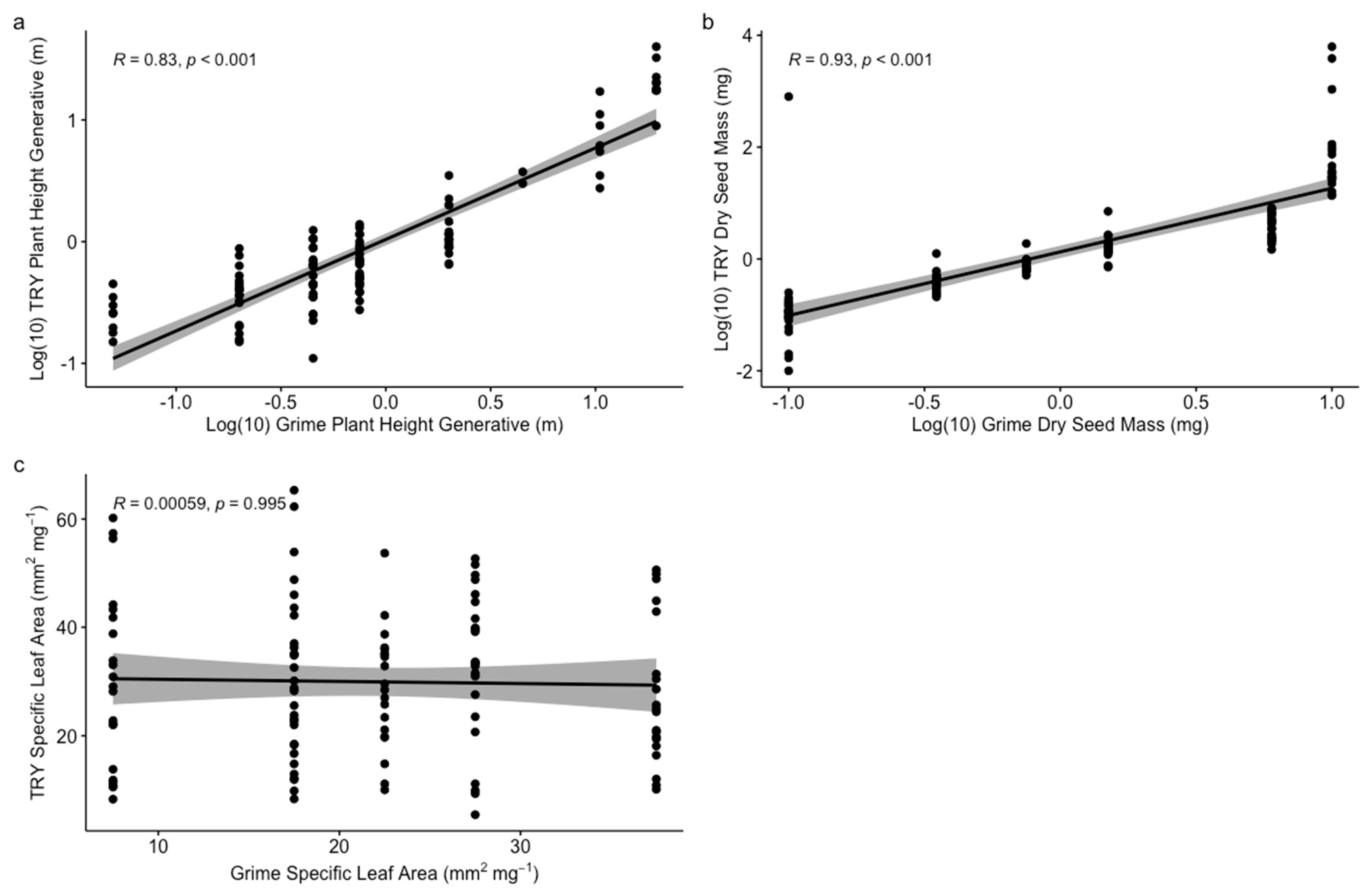
3.1. Trait Validation and Overall Functional and Taxonomic Dissimilarity

Figure 4 shows results from our test of concordance between trait data from different sources (see Section 2.2, above), in which we carried out Spearman’s rank correlations between ordinal data from Grime et al. [87] and the equivalent, continuous trait data from the TRY database. The data correlated well for log(10) plant height and log(10) seed mass, but there was no correlation for SLA.

We found a high level of total dissimilarity between site pairs (i.e., each disturbed site and its twin undisturbed site), driven by a high rate of turnover and low nestedness for both FD and TD (Figure 5). The mean turnover and total dissimilarity were generally higher and nestedness was lower for taxonomic than for functional nestedness.

3.2. Time since Disturbance

Again, using site pairs (each disturbed site and its undisturbed twin), we found little effect of time since disturbance (

Table 4. Results of two-way ANOVAs with years (2016, 2017 and 2019) and β-type (functional or taxonomic) as fixed factors and dissimilarity between site pairs (twinned disturbed and undisturbed sites) as response variables. Note that although partitioned components are referred to as “turnover” and “nestedness”, taxonomic abundance dissimilarity calculated using the Ruzicka and Bray–Curtis indices actually calculates balanced variation in abundance (analogous to turnover) and abundance gradients (analogous to nestedness-resultant components). Significance is indicated by * p ≤ 0.05 and *** p ≤ 0.001.

Partitioned Component	Fixed Factors	df	Error df	F	p
Jaccard Turnover	Year	1	108	0.595	0.442
	Beta type	1	108	29.028	0.000	***
	Year: Beta type	1	108	1.138	0.288
Jaccard Nestedness	Year	1	108	1.133	0.290
	Beta type	1	108	12.891	0.000	***
	Year: Beta type	1	108	4.928	0.029	*
Jaccard Total	Year	1	108	0.022	0.883
	Beta type	1	108	33.621	0.000	***
	Year: Beta type	1	108	1.289	0.259
Sørensen Turnover	Year	1	108	0.627	0.430
	Beta type	1	108	27.881	0.000	***
	Year: Beta type	1	108	1.224	0.271
Sørensen Nestedness	Year	1	108	1.228	0.270
	Beta type	1	108	6.683	0.011	*
	Year: Beta type	1	108	6.487	0.012	*
Sørensen Total	Year	1	108	0.013	0.910
	Beta type	1	108	32.118	0.000	***
	Year: Beta type	1	108	0.952	0.331

; Figure S2). A two-way ANOVA with β-type and partitioned components found significant differences between FD and TD means. The mean turnover was significantly higher (p < 0.001) than mean nestedness for both β-types for both indices. No significant differences between pairwise β-types for year means (2016, 2017 and 2019) were found (Table 4). Weak but marginally significant interaction effects between β-type and year were, however, observed for nestedness-resultant components, meaning that differences in nestedness between β-types were influenced slightly by the time since disturbance.

3.3. Dissimilarity within Each Disturbance Treatment

We found significant differences between the centroids (

Table 5. Mean (centroid) group values for total beta and partitioned component centroids from dissimilarity matrices with one standard error (SE). All values are rounded to three decimal places. Treatment refers to disturbed versus undisturbed dissimilarity matrices and beta type refers to taxonomic versus functional dissimilarity matrices. Note that although partitioned components are referred to as “turnover” and “nestedness” (short for nestedness-resultant), the taxonomic abundance beta calculated using the Ruzicka and Bray–Curtis indices actually calculates balanced variation in abundance (analogous to turnover) and abundance gradients (analogous to nestedness-resultant components).

Treatment	Mean Disturbed	SE	Mean Undisturbed	SE
Jaccard/Ruzicka Turnover	0.732	0.003	0.735	0.003
Jaccard/Ruzicka Nestedness	0.569	0.005	0.508	0.005
Jaccard/Ruzicka Total dissimilarity	0.888	0.002	0.834	0.002
Sørensen/Bray–Curtis Turnover	0.297	0.004	0.228	0.003
Sørensen/Bray–Curtis Nestedness	0.186	0.003	0.105	0.002
Sørensen/Bray–Curtis Total dissimilarity	0.819	0.002	0.734	0.002
Beta Diversity Type	Mean Taxonomic	SE	Mean Functional	SE
Jaccard/Ruzicka Turnover	0.588	0.003	0.879	0.001
Jaccard/Ruzicka Nestedness	0.210	0.003	0.867	0.002
Jaccard/Ruzicka Total dissimilarity	0.798	0.002	0.923	0.001
Sørensen/Bray–Curtis Turnover	0.460	0.003	0.066	0.001
Sørensen/Bray–Curtis Nestedness	0.226	0.003	0.066	0.001
Sørensen/Bray–Curtis Total dissimilarity	0.686	0.002	0.867	0.002

) of disturbance treatments for all components of dissimilarity except Jaccard/Ruzicka turnover (

Table 6. Results of permutation-based two-way ANOVAs with treatment (disturbed sites versus undisturbed sites) and β-type (functional or taxonomic) as fixed factors and dissimilarity matrices of partitioned pairwise β as the response variables with 999 permutations. Note that although partitioned components are referred to as “turnover” and “nestedness” (short for nestedness-resultant), the taxonomic abundance β calculated using the Ruzicka and Bray–Curtis indices actually calculates the balanced variation in abundance (analogous to turnover) and abundance gradients (analogous to nestedness-resultant components). Significance is indicated by * p ≤ 0.05, ** p ≤ 0.01 and *** p ≤ 0.001.

Partitioned Component	Fixed Factors	df	Error	F-Value	p-Value	Sig.
Jaccard/Ruzicka Turnover	Treatment	1	12,316	0.574	0.455
	Beta type	1	12,316	7099.02	0.000	***
	Treatment: Beta type	1	12,316	30.142	0.000	***
Jaccard/Ruzicka Nestedness	Treatment	1	12,316	387.044	0.001	***
	Beta type	1	12,316	44,128.5	0.001	***
	Treatment: Beta type	1	12,316	30.753	0.001	***
Jaccard/Ruzicka Total	Treatment	1	12,316	733.303	0.001	***
	Beta type	1	12,316	3925.17	0.001	***
	Treatment: Beta type	1	12,316	10.496	0.003	**
Sørensen/Bray–Curtis	Treatment	1	12,316	387.840	0.001	***
	Beta type	1	12,316	12,684.1	0.001	***
	Treatment: Beta type	1	12,316	103.950	0.001	***
Sørensen/Bray–Curtis	Treatment	1	12,316	728.272	0.001	***
Nestedness	Beta type	1	12,316	2868.25	0.001	***
	Treatment: Beta type	1	12,316	62.265	0.001	***
Sørensen/Bray–Curtis Total	Treatment	1	12,316	926.226	0.001	***
	Beta type	1	12,316	4200.59	0.001	***
	Treatment: Beta type	1	12,316	4.479	0.034	*

), with greater dissimilarity among disturbed sites than among undisturbed sites.

A null model with 999 permutations indicated that the results for undisturbed sites were not distinguishable from the random expectation of functional diversity (standardised effect size = –0.277 from randomly shuffling species). In contrast, the functional diversity for disturbed sites was significantly higher than expected from the null model (standardised effect size = 2.626; Figure 6).

3.4. Effects of Environmental Variables

We found little evidence for effects of environmental variables in this dataset (

Table 7. Mantel tests of pairwise dissimilarity calculated using the “vegan” package in R with Pearson’s correlation. Functional and taxonomic abundance beta diversity were calculated using partitioned Sørensen (and Bray–Curtis, which is equivalent to Sørensen for abundance) and Jaccard (and Ruzicka which is equivalent to Jaccard for abundance data) indices. The resulting total dissimilarity, turnover and nestedness-resultant distance matrices were correlated with distance matrices for canopy cover (%) and geographical distance. Values provided are Mantel’s r, with significance indicated as * 0.05 > p > 0.01, *** p = 0.001. p values were derived from 9999 permutations using Pearson’s Correlation.

Dissimilarity Measure	Notation	Canopy Cover		Geographic Distance
Functional Diversity		Mantel’s r	p	Mantel’s r	p
Total Sørensen dissimilarity	βsor	−0.07253	0.989	0.007229	0.358
Simpson (Turnover)	βsim	−0.05412	0.885	0.06611 *	0.018
Nestedness (Sørensen)	Βsne	0.01832	0.333	−0.06292	0.982
Total Jaccard dissimilarity	βjac	−0.06862	0.990	0.006352	0.371
Turnover (Jaccard)	βjtu	−0.05653	0.899	0.06962 *	0.014
Nestedness (Jaccard)	βjne	0.03228	0.217	−0.06837	0.991
Taxonomic (abundance) diversity
Total Bray–Curtis dissimilarity	βbray	−0.02003	0.708	0.05349 *	0.049
Turnover equivalent (Bray–Curtis)	βbray_bal	0.03625	0.111	0.08619 ***	0.000
Nestedness equivalent (Bray–Curtis)	βbray_gra	−0.05267	0.921	−0.04825	0.973
Total Ruzicka dissimilarity	βruz	−0.0163	0.674	0.04805 *	0.036
Turnover equivalent (Ruzicka)	βruz_bal	0.03711	0.095	0.07966 ***	0.000
Nestedness equivalent (Ruzicka)	βruz_gra	−0.04767	0.921	−0.06576	0.997

). All correlations between canopy cover and functional dissimilarity were not significantly different from zero. The same was true for correlations between canopy cover and taxonomic dissimilarity. For geographic distance, all correlations were, again, close to zero, but those for turnover were significantly positive (Table 7)—that is, sites further apart tended to have slightly higher turnover (both functional and taxonomic) than those closer together. These results are robust to correlation methods (very similar for Spearman’s rank correlation).

3.5. Invasion Status and Life-Form

Most plant life forms were approximately equally distributed between disturbed and undisturbed sites (Figure 7). The two significant exceptions were phanerophytes, which were more often found in undisturbed sites, and therophytes, which were more often found in undisturbed sites.

Regarding invasion status, we found no significant differences (Chi²(2, 190) = 0.585, p = 0.746) between disturbed and undisturbed sites in occurrences of neophytes, archaeophytes and natives. Occurrences of neophytes (i.e., more recently introduced species) were low throughout (6.32% of occurrences in disturbed sites and 9.47% of occurrences in undisturbed sites).

4. Discussion

This study aimed to utilize the pseudo-experimental setting offered by canal bank engineering to better understand drivers of community assembly. Specifically, we focused on dissimilarities (beta diversity, β) between disturbed and undisturbed plant communities and dissimilarities between communities within each of these treatments. We found high levels of taxonomic (85–90%) and functional (70–76%) dissimilarities between disturbed and undisturbed sites, which were primarily driven by turnover (Figure 5). This first finding aligns with many previous, relevant small-scale studies that found a high level of total dissimilarity between disturbed and undisturbed sites [25,26,27,116] (Table S1). While dissimilarities between disturbed and undisturbed communities were primarily driven by turnover for both taxonomic-β and functional-β, the relative nestedness component was larger for functional-β. A nestedness-dominated β is more commonly attributed to stronger environmental gradients than those in this study [117] (Table S1). Within the treatments, the disturbed sites had greater between-site taxonomic and functional dissimilarities and a lower plant abundance than undisturbed sites, driven by both turnover and nestedness components. The disturbed site functional diversity diverged strongly from null expectations, while the undisturbed site functional diversity did not. These within-treatment findings suggest positive contributions of disturbances to biodiversity. The following sections discuss these main findings in more detail.

4.1. Taxonomic-β and Functional-β

At small scales, a very simplified framework for viewing the impact of disturbance is that net decreases in β (producing more similar community compositions) occur via the environmental filtering of disturbance-tolerant communities, whereas increases in β (producing more distinct communities) occur via processes of competitive biotic interactions. However, in either scenario, the net β is also influenced by factors such as community biomass, spatial scale and the regional species pool [13]. For taxonomic diversity, we found a high level of total dissimilarity between disturbed and undisturbed site pairs (Figure 5) and higher level of dissimilarity between disturbed sites (i.e., within treatment) than between undisturbed sites (Table 5). Previous small-scale studies have, as noted herein, reported high taxonomic-β driven by turnover following a disturbance [25,118]. For instance, a study quantifying taxonomic-β in semi-arid woodlands of varying burn severity concluded that the taxonomic-β was primarily driven by turnover at all levels of burn severity. In that case, the highest taxonomic-β was found at the lowest burn severity level and β decreased with disturbance (burn) intensity [116].

At very small spatial scales (e.g., 1 m²), disturbed and undisturbed site pairs may be expected to display a high level of dissimilarity (driven by turnover, as seen in this study) because of three key factors: a low level of species richness, stochastic dispersal and inter- and intra-species interactions. The additive partitioning of pairwise β using the Sørensen or Jaccard indices (or their abundance equivalents) limits turnover to the species richness of the less-diverse site [18]. A dissimilarity involving disturbed sites, with their lower mean species richness (Figure 3), is more likely to be associated with a higher pairwise dissimilarity through a sampling effect. Therefore, the low species richness of the disturbed sites may partly explain the high pairwise turnover and level of total dissimilarity displayed in this study. Although its effect is often tested using null models [119], a low level of species richness producing β patterns is almost never discussed in papers partitioning β (however, see [13]) and may affect null model interpretation. Equally, the impact of low levels of species richness producing a high level of total-dissimilarity via turnover should be considered by assessing β patterns at a range of scales in future studies [120].

The small-scale random dispersal of founding species has been shown to affect subsequent species identities via facilitation or inhibition, increasing between-site β [27]. Dispersal effects may be particularly strong in highly fragmented urban habitats (such as those surrounding the Basingstoke Canal in this study), where the dispersal of invasive ornamental and competitive species can increase taxonomic diversity [5,121] and has been shown to produce higher turnover [122]. The stochasticity of the colonisation of disturbed sites may be related to the fluctuating resource availability hypothesis [123]. Under this hypothesis, communities are more vulnerable to colonisation by invasive (and native) species when limiting resources are underutilised, e.g., post disturbance [123]. However, in this study, there were low numbers of invasive species recorded in disturbed and undisturbed sites (6.32% and 9.47% neophytes respectively; not significantly different). The low numbers were perhaps due to the dominance of the small-scale stochastic effects of seedling establishment not providing the invasive species with competitive advantages, as found in a study on understory seedling establishment in Poland [124]. The results of this study are therefore consistent with invasive species being the products (as opposed to drivers) of disturbances.

Disturbances may act to filter both native and invasive plant traits [125,126,127] and therefore provide a low contribution to the total β in urbanised riparian vegetation [24]. Under the successional theory, disturbances may also favour initial recolonisation by annual therophytes as opposed to perennial phanerophytes, consistent with this study (Figure 7). Thus, the proportions of invasive and native life-forms in the regional species pool may affect community invasive species proportions [128] and therefore β. Variable relationships between disturbance mechanisms (and scales), species pool characteristics and resource availability release [129] may therefore explain the highly variable correlations of invasive species with anthropogenic disturbances within the literature [130,131,132]. Additionally, a recent metanalysis found that at low level of dispersal, a disturbance increased β compared with a high level of dispersal for which the disturbance had a homogenising effect [133]. Both patterns observed by Catano et al. [133] displayed scale dependence, suggesting that the variable dispersal capacity may affect the observed β in this study.

A small-scale (1 m²) experimental study excluding dispersal concluded that β increased under species competitive exclusions in seeding experiments but decreased in species removal experiments [134]. Biotic interactions might therefore increase between-site heterogeneity via competitive exclusions [41], possibly explaining the high levels of dissimilarity and turnover in this study. However, biotic interactions depend on the initial starting community [28]. In this study, it was expected that as species abundance increases from the initial disturbance year (2016) to undisturbed sites, the relative role of biotic interactions in driving taxonomic dissimilarity would increase [120]. However, the post-disturbance year did not significantly affect β. The sampling period in this study (four years) may have been too short for biotic effects to become dominant. For example, although more isolated (~1 km from intact plant communities), a study on mudflow plant succession (similar to the disturbance regime in this study, with the complete removal of above and belowground biomass) found strong initial effects of probabilistic dispersal on community composition [135]. Biotic interactions only became important later in the 20-year sampling period [135]. Therefore, stochastic dispersal may better explain observed taxonomic turnover in this study, and longer-term studies may be needed to better understand how partitioned taxonomic-β changes through time according to community assembly processes [7].

Although we found high level of total dissimilarity in functional diversity, driven primarily by turnover (Figure 5; Table 5), both were significantly lower than the equivalent measures for taxonomic diversity. The nestedness component was larger, relatively, for functional diversity than for taxonomic diversity. The overall dissimilarity patterns were nonetheless broadly consistent between functional and taxonomic diversity. This consistency is in line with previous post-disturbance studies and is expected because the loss (or gain) of species typically brings the loss (or gain) of functional traits [24,136]. However, functional redundancy or environmental filtering can decouple functional and taxonomic diversity [41]. A higher level of functional nestedness relative to taxonomic nestedness has been recorded in previous studies [137,138]. For example, a depth gradient produced a higher level of small-scale (transect) functional nestedness in lake macrophytes compared with higher taxonomic turnover [118]. Similarly, Fukami et al. [27] reported small-scale functional convergence over time due to environmental filtering, while the taxonomic-β was constant. The higher levels of relative functional nestedness in this study may be due to fewer functional strategies than species identities (and abundances) being able to persist in towpath plant communities. These communities must cope with a high degree of shading, hydric soil conditions and a high degree of disturbance (e.g., via engineering, annual vegetation cutback or trampling; Basingstoke Canal Authority, personal communication, June 2020). However, contrary to previous studies, we did not find nestedness-dominated functional convergence in this study.

We found no significant change in functional nestedness or turnover (functional convergence or divergence) across years. Varying functional drivers can be explained by turnover due to dispersal limitations and environmental heterogeneity between sites, while nestedness is typically associated with a gradual loss of functions over environmental gradients [139]. Processes operating to regulate functional-β are therefore complex and multidirectional. Additionally, β displays almost no correlation with geographic distance or shading, meaning that patterns are not spatially or environmentally structured by variables recorded in this study (Table 7). The non-environmentally structured β differs from the previous literature. For example, a macroinvertebrate mesocosm-based drought intensification experiment found that taxonomic dissimilarity was driven by turnover and functional-β was driven by varying turnover and nestedness along the disturbance gradient [140]. Spatial and environmental structuring of taxonomic-β and functional-β are often seen at larger spatial scales [117,138,141,142]. For example, a study on fire disturbances concluded that half of the (high) taxonomic-β and functional-β, driven primarily by turnover, was explained by spatial and environmental variables [26]. However, small spatial scales (this study) are thought to be more influenced by biotic interactions operating at the individual plant scale (~0.04 m²; [134]). Individuals can alter the functional traits and identities of surrounding species. Biotic competition drives multi-directional processes of functional divergence and indirect facilitation via resource partitioning (e.g., in a small-scale study of semi-arid Mediterranean shrub communities [6]). Post-disturbance release from competition and more underutilised resources may also result in more viable functional strategies for coexistence, increasing functional turnover [12,143]. For example, Stępień et al. [144] recorded rapid post-dredging recovery to pre-disturbance levels (~2 years) for temperate riparian vegetation. Initial succession by ruderal therophytes and invasive species with distinct functional traits was followed by an increase in pre-disturbance species in the second year of succession [144]. Therefore, similarly to taxonomic-β, the high levels of functional-β in this study, driven primarily by turnover, might be primarily explained by stochastic biotic interactions driven by probabilistic initial community assemblages, with additional increases in viable functional strategies in disturbed sites.

4.2. Uncertainty of Functional Diversity

The functional-β value was calculated from global databases, which may not represent local trait values well [145]. Validation analyses using ordinal UK and continuous global trait data found strong correlations across the databases for plant height and seed mass (Figure 4). This concordance suggests that the conclusions drawn for these traits may be robust to the source of the trait data. However, SLA displayed almost no correlation between databases, probably because of the relatively high intra-specific variation of SLA and because small amounts of spatial or sampling variation in leaf area or dry mass values can dramatically shift SLA values [146,147]. For example, in Kazakou et al. [148], the experimental addition of soil nitrogen resulted in a greater variation in SLA than plant height or seed mass. Further, a study found significant bias towards higher values in all three traits in the TRY database [149]. The bias resulted from many factors, including that roadside plants may be preferentially sampled and have higher SLA due to higher soil nitrogen concentrations. Therefore, multiple-trait FD using secondary data, both in this study and in other β-partitioning studies (e.g., [118,142]), may not be very locally representative. Thus, there could be some over- or under-estimation of dissimilarity between sites [42]. Future research should therefore ideally collect in situ trait data where appropriate (e.g., SLA). For plant height, however, the age of the plant is typically a key determinant for a plant measured in situ. Directly measuring height would therefore be inappropriate for studying community assembly (in which the plant strategy is the main focus), especially when (as here) the treatments differ in the time since disturbance. Instead, the normal maximum height of mature individuals of each species should be used, a purpose for which trait databases are appropriate.

4.3. Disturbed versus Undisturbed β

The disturbed sites had significantly higher levels of dissimilarity (total, turnover and nestedness) than undisturbed sites for both taxonomic and functional diversity (Table 4). Additionally, there was a small but significant interaction for disturbed sites, meaning that the effect of disturbance treatment depends on the β-type. Higher post-disturbance β values, driven primarily by turnover, have been recorded in many previous studies [25,116,118]. However, in this study, the significantly lower species abundances in disturbed sites could partially explain the higher turnover and total dissimilarity (Figure 3).

Due to the variable impact of species richness patterns in driving total community dissimilarity, null models are needed to determine whether (at fixed observed species abundances) the functional-β of disturbed sites differs from random expectation [114]. Our null model found much higher levels of dissimilarity of traits in disturbed communities than what was expected by chance (Figure 6). At the 1 m² spatial grain of this study, it could be expected that disturbed site trait dissimilarities are attributable to stochastic biotic interactions. As reported in the previous literature (e.g., experimental seeding experiments [134]), stochastic interactions can be explained by the “limiting similarity” theory in which competing species functionally diverge to facilitate coexistence [120,150,151]. However, these patterns may be better explained by dispersal or deterministic environmental heterogeneity (e.g., variable disturbed soil properties) driving high stochastic turnover. Functional nestedness could be produced from a subset of species with a high dispersal capacity or generalist traits suitable for a range of environmental conditions at the spatial extent of this study (~50 km [7]). For example, a study comparing temporary versus permanent wetland taxa recorded high plant β driven primarily by turnover in more disturbed temporary wetlands, with weaker nestedness components that were probably due to a nested subset of disturbance-tolerant species [117].

Given the industrial history of UK canals, dredged soil materials in disturbed sites are likely to contain spatially heterogenous, elevated nutrient concentrations and contaminants such as heavy metals and pesticides [152,153]. Pollutants may produce more spatially heterogenous environmental filters in disturbed sites, resulting in observed trait divergence compared with relative convergence in undisturbed sites (Figure 6). This is consistent with disturbed sites being strongly characterised by Juncus effusus, which has high heavy-metal tolerance [154]. However, the scale dependence of community drivers found in previous research means that patterns of functional diversity in relation to null expectation in this study may change at larger scales [16,155].

4.4. Performance of β Indices

Overall, the Sørensen (or Bray–Curtis) and Jaccard (or Ruzicka) indices resulted in very similar patterns of β. However, the differential weighting of shared species between the indices (with β_sor measuring the proportion of unique species per site and β_jac measuring the unique species within the species pool by double-weighting shared species) means that when the relative turnover is less than the total dissimilarity (as in this study), β_sor and β_sim will be lower but not maximally differentiated from β_jac and β_jtu (Table 3; [98,156]). When using hard-boundary significance thresholds (e.g., p < 0.05), small numerical differences between indices, which may not be ecologically relevant, can lead to differences in overall significance and therefore alter the conclusions drawn. For example, the functional turnover and taxonomic turnover were significantly different between the disturbed and undisturbed sites using the Sørensen indices, but no significant difference was found for Jaccard (Table 6). Importantly, in permutation-tests, the p-values themselves are sensitive to the number of permutations run [157]. Additionally, in PERMANOVAs, Sørensen produced significantly higher mean taxonomic turnover values than values for functional turnover and functional nestedness, whereas Jaccard produced the opposite pattern. In the previous literature, Sørensen was perhaps more popular simply due to its initial presentation by Baselga [48]. However, studies partitioning β using either the Jaccard [139] or Sørensen [24,25,49,116,118,142] indices without checking the robustness of results to methodological decisions may interpret ecologically identical conclusions as being distinct. From a broader perspective, this study highlights support for the use of significance values as measures of context-specific statistical clarity instead of hard boundaries [158,159,160], particularly in ecological science where biological significance may not relate directly to statistical significance [161].

5. Conclusions

Few studies have applied the partitioning of functional-β and taxonomic-β to post-disturbance communities [24]. Our study, which carried out this partitioning for canal-bank plant communities disturbed by bank engineering work, indicates that such small-scale disturbances may increase taxonomic and functional dissimilarity in anthropogenic habitats without invasive species increases. In disturbance regimes where above and below-ground biomass is removed (as here), communities may be primarily structured by random dispersal from the regional species pool. Diversity driven by turnover will promote locally rare species or functions, whereas within nested communities, only the richest biotas contain rare species or functions. Therefore, partitioning is informative for conservation. Our results lend support for local-scale conservation that enhances habitat heterogeneity to promote taxonomic diversity and its corresponding biotic functions. The results are consistent with invasive species as “passengers” instead of drivers of diversity change, with disturbances releasing resources and producing equal colonisation opportunities for both native and invasive species [123]. Therefore, although some invasive species are particularly problematic, overall conservation may be better placed to promote biodiversity via assessing the role of anthropogenic disturbances instead of invasive species [24]. Finally, this study demonstrates the importance of considering how methodological choices affect results in community assembly studies.

References

1. Hooke, R.L.; Martín-Duque, J.F. Land transformation by humans: A review. Geol. Soc. Am. 2012, 22, 4–10. Available online: https://www.geosociety.org/gsatoday/archive/22/12/abstract/i1052-5173-22-12-4.htm (accessed on 5 March 2023). [CrossRef]
2. Woodwell, G. The Earth in Transition: Patterns and Processes of Biotic Impoverishment; Cambridge University Press: Cambridge, UK, 1991. [Google Scholar] [CrossRef]
3. McKinney, M.L. Urbanization, Biodiversity, and Conservation: The impacts of urbanization on native species are poorly studied, but educating a highly urbanized human population about these impacts can greatly improve species conservation in all ecosystems. BioScience 2002, 52, 883–890. [Google Scholar] [CrossRef]
4. Pickett, S.T.A.; White, P. The Ecology of Natural Disturbance and Patch Dynamics; Academic Press: San Diego, CA, USA; London, UK, 1985. [Google Scholar]
5. McKinney, M.L.; Lockwood, J.L. Biotic homogenization: A few winners replacing many losers in the next mass extinction. Trends Ecol. Evol. 1999, 14, 450–453. [Google Scholar] [CrossRef] [PubMed]
6. Chacón-Labella, J.; de la Cruz, M.; Pescador, D.S.; Escudero, A. Individual species affect plant traits structure in their surroundings: Evidence of functional mechanisms of assembly. Oecologia 2016, 180, 975–987. [Google Scholar] [CrossRef]
7. Götzenberger, L.; de Bello, F.; Bråthen, K.A.; Davison, J.; Dubuis, A.; Guisan, A.; Leps, J.; Lindborg, R.; Moora, M.; Pärtel, M.; et al. Ecological assembly rules in plant communities-approaches, patterns and prospects. Biol. Rev. 2011, 87, 111–127. [Google Scholar] [CrossRef]
8. Schmidt, V.T.; Smith, K.F.; Melvin, D.W.; Amaral-Zettler, L.A. Community assembly of a euryhaline fish microbiome during salinity acclimation. Mol. Ecol. 2015, 24, 2537–2550. [Google Scholar] [CrossRef] [PubMed]
9. Troia, M.J.; Gido, K.B. Functional strategies drive community assembly of stream fishes along environmental gradients and across spatial scales. Oecologia 2015, 177, 545–559. [Google Scholar] [CrossRef]
10. Kroll, A.J.; Verschuyl, J.; Giovanini, J.; Betts, M.G. Assembly dynamics of a forest bird community depend on disturbance intensity and foraging guild. J. Appl. Ecol. 2017, 54, 784–793. [Google Scholar] [CrossRef]
11. Montaño-Centellas, F.A.; McCain, C.; Loiselle, B.A. Using functional and phylogenetic diversity to infer avian community assembly along elevational gradients. Glob. Ecol. Biogeogr. 2020, 29, 232–245. [Google Scholar] [CrossRef]
12. Grime, J.P. Trait convergence and trait divergence in herbaceous plant communities: Mechanisms and consequences. J. Veg. Sci. 2006, 17, 255–260. [Google Scholar] [CrossRef]
13. Myers, J.A.; Chase, J.M.; Crandall, R.M.; Jiménez, I. Disturbance alters beta-diversity but not the relative importance of community assembly mechanisms. J. Ecol. 2015, 103, 1291–1299. [Google Scholar] [CrossRef]
14. Poos, M.S.; Walker, S.C.; Jackson, D.A. Functional-diversity indices can be driven by methodological choices and species richness. Ecology 2009, 90, 341–347. [Google Scholar] [CrossRef]
15. McGill, B.J. Towards a unification of unified theories of biodiversity. Ecol. Lett. 2010, 13, 627–642. [Google Scholar] [CrossRef] [PubMed]
16. Smith, A.B.; Sandel, B.; Kraft, N.J.B.; Carey, S. Characterizing scale-dependent community assembly using the functional-diversity–area relationship. Ecology 2013, 94, 2392–2402. [Google Scholar] [CrossRef] [PubMed]
17. Rosenblad, K.C.; Sax, D.F. A new framework for investigating biotic homogenization and exploring future trajectories: Oceanic island plant and bird assemblages as a case study. Ecography 2016, 39, 1040–1049. [Google Scholar] [CrossRef]
18. Villéger, S.; Grenouillet, G.; Brosse, S. Decomposing functional β-diversity reveals that low functional β-diversity is driven by low functional turnover in European fish assemblages. Glob. Ecol. Biogeogr. 2013, 22, 671–681. [Google Scholar] [CrossRef]
19. Bromhead, J.C.; Beckwith, P. Environmental Dredging on the Birmingham Canals: Water Quality and Sediment Treatment. Water Environ. J. 1994, 8, 350–359. [Google Scholar] [CrossRef]
20. Singh, S.P.; Tack, F.M.G.; Verloo, M.G. Extractability and bioavailability of heavy metals in surface soils derived from dredged sediments. Chem. Speciat. Bioavailab. 1996, 8, 105–110. [Google Scholar] [CrossRef]
21. Hoosein, S. Soil Properties Affect Establishment of Invasive Species, Celastrus orbiculatus, in a Lower Hudson River Riparian Ecosystem. Master’s Thesis, State University of New York at Albany, Albany, NY, USA, 2016. [Google Scholar]
22. Mayer, K.; Haeuser, E.; Dawson, W.; Essl, F.; Kreft, H.; Pergl, J.; Pyšek, P.; Weigelt, P.; Winter, M.; Lenzner, B.; et al. Naturalization of ornamental plant species in public green spaces and private gardens. Biol. Invasions 2017, 19, 3613–3627. [Google Scholar] [CrossRef]
23. Olden, J.D.; Poff, N.L. Toward a mechanistic understanding and prediction of biotic homogenization. Am. Nat. 2003, 162, 442–460. [Google Scholar] [CrossRef]
24. Brice, M.-H.; Pellerin, S.; Poulin, M. Does urbanization lead to taxonomic and functional homogenization in riparian forests? Divers. Distrib. 2017, 23, 828–840. [Google Scholar] [CrossRef]
25. Alignier, A.; Baudry, J. Is plant temporal beta diversity of field margins related to changes in management practices? Acta Oecologica 2016, 75, 1–7. [Google Scholar] [CrossRef]
26. Freeman, J.E.; Kobziar, L.N.; Leone, E.H.; Williges, K. Drivers of plant functional group richness and beta diversity in fire-dependent pine savannas. Divers. Distrib. 2019, 25, 1024–1044. [Google Scholar] [CrossRef]
27. Fukami, T.; Bezemer, M.T.; Mortimer, S.R.; Putten, W.H. Species divergence and trait convergence in experimental plant community assembly. Ecol. Lett. 2005, 8, 1283–1290. [Google Scholar] [CrossRef]
28. Smart, S.M.; Thompson, K.; Marrs, R.H.; Le Duc, M.G.; Maskell, L.C.; Firbank, L.G. Biotic homogenization and changes in species diversity across human-modified ecosystems. Proc. R. Soc. B Biol. Sci. 2006, 273, 2659–2665. [Google Scholar] [CrossRef]
29. Hulme, P.E.; Bremner, E.T. Assessing the impact of Impatiens glandulifera on riparian habitats: Partitioning diversity components following species removal. J. Appl. Ecol. 2006, 43, 43–50. [Google Scholar] [CrossRef]
30. Condit, R.; Pitman, N.; Leigh, E.G.; Chave, J.; Terborgh, J.; Foster, R.B.; Nuñez, P.; Aguilar, S.; Valencia, R.; Villa, G.; et al. Beta-diversity in tropical forest trees. Science 2002, 295, 666–669. [Google Scholar] [CrossRef]
31. Jaccard, P. The distribution of the flora in the alpine zone. New Phytol. 1912, 11, 37–50. [Google Scholar] [CrossRef]
32. Simpson, G.G. Mammals and the nature of continents. Am. J. Sci. 1943, 241, 1–31. [Google Scholar] [CrossRef]
33. Sørensen, T.A. A method of establishing groups of equal amplitude in plant sociology based on similarity of species content, and its application to analyses of the vegetation on Danish commons. K. Dan. Vidensk. Selsk. Biol. Skr. 1948, 5, 1–34. [Google Scholar]
34. Whittaker, R.H. Vegetation of the Siskiyou Mountains, Oregon and California. Ecol. Monogr. 1960, 30, 280–338. [Google Scholar] [CrossRef]
35. Jost, L. Partitioning diversity into independent alpha and beta components. Ecology 2007, 88, 2427–2439. [Google Scholar] [CrossRef] [PubMed]
36. Chao, A.; Chiu, C.-H.; Hsieh, T.C. Proposing a resolution to debates on diversity partitioning. Ecology 2012, 93, 2037–2051. [Google Scholar] [CrossRef] [PubMed]
37. Socolar, J.B.; Gilroy, J.J.; Kunin, W.E.; Edwards, D.P. How Should Beta-Diversity Inform Biodiversity Conservation? Trends Ecol. Evol. 2016, 31, 67–80. [Google Scholar] [CrossRef] [PubMed]
38. Cortina, J.; Maestre, F.T.; Vallejo, R.; Baeza, M.J.; Valdecantos, A.; Pérez-Devesa, M. Ecosystem structure, function, and restoration success: Are they related? J. Nat. Conserv. 2006, 14, 152–160. [Google Scholar] [CrossRef]
39. Díaz, S.; Lavorel, S.; de Bello, F.; Quétier, F.; Grigulis, K.; Robson, M. Incorporating plant functional diversity effects in ecosystem service assessments. Proc. Natl. Acad. Sci. USA 2007, 104, 20684–20689. [Google Scholar] [CrossRef]
40. Villéger, S.; Mason, N.W.H.; Mouillot, D. New multidimensional functional diversity indices for a multifaceted framework in functional ecology. Ecology 2008, 89, 2290–2301. [Google Scholar] [CrossRef]
41. Mayfield, M.M.; Bonser, S.P.; Morgan, J.W.; Aubin, I.; McNamara, S.; Vesk, P.A. What does species richness tell us about functional trait diversity? Predictions and evidence for responses of species and functional trait diversity to land-use change. Glob. Ecol. Biogeogr. 2010, 19, 423–431. [Google Scholar] [CrossRef]
42. Lavorel, S.; Grigulis, K.; McIntyre, S.; Williams, N.S.G.; Garden, D.; Dorrough, J.; Berman, S.; Quétier, F.; Thébault, A.; Bonis, A. Assessing functional diversity in the field—Methodology matters! Funct. Ecol. 2008, 22, 134–147. [Google Scholar] [CrossRef]
43. Swenson, N.G.; Anglada-Cordero, P.; Barone, J.A. Deterministic tropical tree community turnover: Evidence from patterns of functional beta diversity along an elevational gradient. Proc. R. Soc. B Biol. Sci. 2011, 278, 877–884. [Google Scholar] [CrossRef]
44. Laureto, L.M.O.; Cianciaruso, M.V.; Samia, D.S.M. Functional diversity: An overview of its history and applicability. Nat. Conserv. 2015, 13, 112–116. [Google Scholar] [CrossRef]
45. Violle, C.; Navas, M.-L.; Vile, D.; Kazakou, E.; Fortunel, C.; Hummel, I.; Garnier, E. Let the concept of trait be functional! Oikos 2007, 116, 882–892. [Google Scholar] [CrossRef]
46. Tuomisto, H. A diversity of beta diversities: Straightening up a concept gone awry. Part 1. Defining beta diversity as a function of alpha and gamma diversity. Ecography 2010, 33, 2–22. [Google Scholar] [CrossRef]
47. Mori, A.S.; Isbell, F.; Seidl, R. β-Diversity, Community Assembly, and Ecosystem Functioning. Trends Ecol. Evol. 2018, 33, 549–564. [Google Scholar] [CrossRef] [PubMed]
48. Baselga, A. Partitioning the turnover and nestedness components of beta diversity. Glob. Ecol. Biogeogr. 2010, 19, 134–143. [Google Scholar] [CrossRef]
49. Baetan, L.; Vangansbeke, P.; Hermy, M.; Peterken, G.; Vanhuyse, K.; Verheyen, K. Distinguishing between turnover and nested-ness in the quantification of biotic homogenization. Biodivers. Conserv. 2012, 21, 1399–1409. [Google Scholar] [CrossRef]
50. Soininen, J.; Heino, J.; Wang, J.A. Meta-analysis of nestedness and turnover components of beta diversity across organisms and ecosystems. Glob. Ecol. Biogeogr. 2018, 27, 96–109. [Google Scholar] [CrossRef]
51. Devictor, V.; Mouillot, D.; Meynard, C.; Jiguet, F.; Thuiller, W.; Mouquet, N. Spatial mismatch and congruence between taxonomic, phylogenetic and functional diversity: The need for integrative conservation strategies in a changing world. Ecol. Lett. 2010, 13, 1030–1040. [Google Scholar] [CrossRef] [PubMed]
52. West, C.; Church, S. The Basingstoke canal: A wildlife survival strategy. Ecos 1991, 12, 40–43. [Google Scholar]
53. Stebbings, R.E. Bats in the Greywell Tunnell, Basingstoke Canal: An Assessment of the Bats in Greywell Tunnel and the Potential Effects on them of the Surrey and Hampshire Canal Society’s Restoration Proposals; Robert Stebbings Consultancy: Peterborough, UK, 1992. [Google Scholar]
54. Pinkett, A.J. Basingstoke canal hydrological study: A water balance. J. Chart. Inst. Water Environ. Manag. 1995, 9, 376–384. [Google Scholar] [CrossRef]
55. Morley, N.J.; Lewis, J.W. Anthropogenic pressure on a molluscan-trematode community over a long-term period in the Basingstoke canal, UK, and its implications for ecosystem health. EcoHealth 2006, 3, 269–280. [Google Scholar] [CrossRef]
56. Ralphs, I.; Callegari, S. Survey of the Wetland Flora of the Basingstoke Canal: Report to the Basingstoke Canal Authority; Hampshire Biodiversity Information Centre: Basingstoke, UK, 2016. [Google Scholar]
57. Tobler, W. A computer movie simulating urban growth in the Detroit region. Econ. Geogr. 1970, 46 (Suppl. 1), 234–240. [Google Scholar] [CrossRef]
58. Jennings, S.B.; Brown, N.D.; Sheil, D. Assessing forest canopies and understorey illumination: Canopy closure, canopy cover and other measures. Forestry 1999, 72, 59–74. [Google Scholar] [CrossRef]
59. Tichý, L.; Gap Light Analysis Mobile Application (Version 3.0). [Mobile App]. 2015. Available online: https://www.sci.muni.cz/botany/glama/GLAMA%20manual.pdf (accessed on 30 June 2020).
60. Bianchi, S.; Cahalan, C.; Hale, S.; Gibbons, J.M. Rapid assessment of forest canopy and light regime using smartphone hemispherical photography. Ecol. Evol. 2017, 7, 10556–10566. [Google Scholar] [CrossRef] [PubMed]
61. Korhonen, L.; Korhonen, K.T.; Rautiainen, M.; Stenberg, P. Estimation of forest canopy cover: A comparison of Weld measurement techniques. Silva Fenn. 2006, 40, 577–588. [Google Scholar] [CrossRef]
62. Public Interest Enterprises. Percentage Cover App (Version 1.0). [Mobile App]. 2017. Available online: https://apps.apple.com/us/app/percentage-cover/id1310190758 (accessed on 30 June 2020).
63. Quintero, C.; Morales, C.L.; Aizen, M.A. Effects of anthropogenic habitat disturbance on local pollinator diversity and species turnover across a precipitation gradient. Biodivers. Conserv. 2009, 19, 257–274. [Google Scholar] [CrossRef]
64. Bosch, J.; Retana, J.; Cerda, X. Flowering phenology, floral traits and pollinator composition in a herbaceous Mediterranean plant community. Oecologia 1997, 109, 583–591. [Google Scholar] [CrossRef]
65. O’Connor, R.S.; Kunin, W.E.; Garratt, M.P.D.; Potts, S.G.; Roy, H.E.; Andrews, C.; Jones, C.M.; Peyton, J.M.; Savage, J.; Harvey, M.C.; et al. Monitoring insect pollinators and flower visitation: The effectiveness and feasibility of different survey methods. Methods Ecol. Evol. 2019, 10, 2129–2140. [Google Scholar] [CrossRef]
66. Carvell, C.; Isaac, N.J.B.; Jitlal, M.; Peyton, J.; Powney, G.D.; Roy, D.B.; Vanbergen, A.J.; O’Connor, R.; Jones, C.; Kunin, B.; et al. Design and Testing of a National Pollinator and Pollination Monitoring Framework; Centre for Ecology & Hydrology: Wallingford, UK.
67. Cane, J.H.; Tepedino, V.J. Causes and extent of declines among native North American invertebrate pollinators: Detection, evidence, and consequences. Conserv. Ecol. 2001, 5, 1. Available online: http://www.consecol.org/vol5/iss1/art1/ (accessed on 5 March 2023). [CrossRef]
68. Nowakowski, M.; Pywell, R.F. Habitat Creation and Management for Pollinators; Centre for Ecology and Hydrology: Wallingford, UK, 2016. [Google Scholar]
69. Jones, H.G. Visual Flora. 2019. Available online: https://visual-flora.org.uk/index.html (accessed on 30 June 2020).
70. Glority Global Group Ltd. PictureThis Mobile Application (2.6.4). [PictureThis]. 2020. Available online: https://www.picturethisai.com/?fbclid=IwAR08UPTQTn7NJX0Y0PVscR92J_KzHtFznfztYFf9KuEHPjCiHTG49lpxeQQ (accessed on 30 June 2020).
71. Hall, C.; Groome, G. 2012 Survey of the wetland flora of the Basingstoke Canal. In Report to Basingstoke Canal Authority; Basingstoke Canal Authority: Mychett, UK, 2013. [Google Scholar]
72. Botanical Society of Britain and Ireland (BSBI). Online Atlas of British and Irish Flora. 2020. Available online: https://www.brc.ac.uk/plantatlas/ (accessed on 30 June 2020).
73. Kumar, N.; Belhumeur, P.N.; Biswas, A.; Jacobs, D.W.; John Kress, W.; Lopez, I.C.; Soares, J.V.B. Leafsnap: A Computer Vision System for Automatic Plant Species Identification. In Lecture Notes in Computer Science, Computer Vision–ECCV 2012: 12th European Conference on Computer Vision, Florence, Italy, 7–13 October 2012; Fitzgibbon, A., Lazebnik, S., Perona, P., Sato, Y., Schmid, C., Eds.; Springer: Berlin/Heidelberg, Germany, 2012; Volume 7573. [Google Scholar] [CrossRef]
74. Bonnet, P.; Goëau, H.; Hang, S.T.; Lasseck, M.; Šulc, M.; Malécot, V.; Jauzein, P.; Melet, J.-C.; You, C.; Joly, A. Plant Identification: Experts vs. Machines in the Era of Deep Learning. In Multimedia Tools and Applications for Environmental and Biodiversity Informatics; Multimedia Systems and Applications; Joly, A., Vrochidis, S., Karatzas, K., Karppinen, A., Bonnet, P., Eds.; Springer: Cham, Switzerland, 2018; pp. 131–149. [Google Scholar] [CrossRef]
75. Weiher, E.; van der Werf, A.; Thompson, K.; Roderick, M.; Garnier, E.; Eriksson, O. Challenging Theophrastus: A common core list of plant traits for functional ecology. J. Veg. Sci. 1999, 10, 609–620. [Google Scholar] [CrossRef]
76. Latzel, V.; Mihulka, S.; Klimešová, J. Plant traits and regeneration of urban plant communities after disturbance: Does the bud bank play any role? Appl. Veg. Sci. 2008, 11, 387–394. [Google Scholar] [CrossRef]
77. Bernhardt-Römermann, M.; Gray, A.; Vanbergen, A.J.; Bergès, L.; Bohner, A.; Brooker, R.W.; De Bruyn, L.; De Cinti, B.; Dirnböck, T.; Grandin, U.; et al. Functional traits and local environment predict vegetation responses to disturbance: A pan-European multi-site experiment. J. Ecol. 2011, 99, 777–787. [Google Scholar] [CrossRef]
78. Herben, T.; Klimešová, J.; Chytrý, M. Effects of disturbance frequency and severity on plant traits: An assessment across a temperate flora. Funct. Ecol. 2018, 32, 799–808. [Google Scholar] [CrossRef]
79. Baselga, A.; Orme, D.; Villéger, S.; De Bortoli, J.; Leprieur, F.; Logez, M.; Henriques-Silva, R.; betapart: Partitioning Beta Diversity into Turnover and Nestedness Components. R Package Version 1.5.2. [Software]. 2020. Available online: https://CRAN.R-project.org/package=betapart (accessed on 4 October 2020).
80. Laughlin, D.C. The intrinsic dimensionality of plant traits and its relevance to community assembly. J. Ecol. 2014, 102, 186–193. [Google Scholar] [CrossRef]
81. Westoby, M. A leaf-height-seed (LHS) plant ecology strategy scheme. Plant Soil 1998, 199, 213–227. [Google Scholar] [CrossRef]
82. Laughlin, D.C.; Leppert, J.J.; Moore, M.M.; Sieg, C.H. A multi-trait test of the leaf-height-seed plant strategy scheme with 133 species from a pine forest flora. Funct. Ecol. 2009, 24, 493–501. [Google Scholar] [CrossRef]
83. Pérez-Harguindeguy, N.; Díaz, S.; Garnier, E.; Lavorel, S.; Poorter, H.; Jaureguiberry, P.; Bret-Harte, M.S.; Cornwell, W.K.; Craine, J.M.; Gurvich, D.E.; et al. New handbook for standardised measurement of plant functional traits worldwide. Aust. J. Bot. 2013, 61, 167–234. [Google Scholar] [CrossRef]
84. Kattge, J.; Bönisch, G.; Díaz, S.; Lavorel, S.; Prentice, I.C.; Leadley, P.; Tautenhahn, S.; Werner, G.D.A.; Aakala, T.; Abedi, M.; et al. TRY plant trait database—Enhanced coverage and open access. Glob. Chang. Biol. 2020, 26, 119–188. [Google Scholar] [CrossRef]
85. Fitter, A.H.; Peat, H.J. The Ecological Flora Database. J. Ecol. 1994, 82, 415–425. [Google Scholar] [CrossRef]
86. Kleyer, M.; Bekker, R.; Knevel, I.; Bakker, J.; Thompson, K.; Sonnenschein, M.; Poschlod, P.; van Groenendael, J.M.; Klimeš, L.; Klimešová, J.; et al. The LEDA Traitbase: A database of life-history traits of the Northwest European flora. J. Ecol. 2008, 96, 1266–1274. [Google Scholar] [CrossRef]
87. Grime, J.P.; Hodgson, J.G.; Hunt, R. Comparative Plant Ecology: A Functional Approach to Common British Species; Unwin Hyman: London, UK, 1988. [Google Scholar]
88. Fern, K. Plants for a Future: Edible and Useful Plants for a Healthier World; Permanent Publications: Hampshire, UK, 1997; ISBN 1-85623-011-2. [Google Scholar]
89. Májeková, M.; Paal, T.; Plowman, N.S.; Bryndová, M.; Kasari, L.; Norberg, A.; Weiss, M.; Bishop, T.R.; Luke, S.H.; Sam, K.; et al. Evaluating Functional Diversity: Missing Trait Data and the Importance of Species Abundance Structure and Data Transformation. PLoS ONE 2016, 11, e0149270. [Google Scholar] [CrossRef]
90. Grime, J.P. Evidence for the existence of three primary strategies in plants and its relevance to ecological and evolutionary theory. Am. Nat. 1977, 111, 1169–1194. [Google Scholar] [CrossRef]
91. Westoby, M.; Falster, D.S.; Moles, A.T.; Vesk, P.A.; Wright, I.J. Plant ecological strategies: Some leading dimensions of variation between species. Annu. Rev. Ecol. Syst. 2002, 33, 125–159. [Google Scholar] [CrossRef]
92. Cornelissen, J.H.C.; Lavorel, S.; Garnier, E.; Díaz, S.; Buchmann, N.; Gurvich, D.E.; Reich, P.B.; Ter Steege, H.; Morgan, H.D.; Van Der Heijden, M.G.A.; et al. A handbook of protocols for standardised and easy measurement of plant functional traits worldwide. Aust. J. Bot. 2003, 51, 335–380. [Google Scholar] [CrossRef]
93. Da Silva, F.C.G. Using Plant Functional Traits to Assess Ecosystem Processes and Community Dynamics in Lowland Fens: Understanding the Efficacy and Applicability of a Trait-Based Approach to Plant Ecology. Ph.D. Thesis, Kingston University, London, UK, 2017. [Google Scholar]
94. Rejmánek, M.; Richardson, D.M. What attributes make some plant species more invasive? Ecology 1996, 77, 1655–1661. [Google Scholar] [CrossRef]
95. Baselga, A.; Orme, C.D.L. betapart: An R package for the study of beta diversity. Methods Ecol. Evol. 2012, 3, 808–812. [Google Scholar] [CrossRef]
96. R Core Team. R: A Language and Environment for Statistical Computing; R Foundation for Statistical Computing: Vienna, Austria, 2020; Available online: https://www.R-project.org/ (accessed on 5 March 2023).
97. RStudio Team. RStudio: Integrated Development for R; RStudio, PBC: Boston, MA, USA, 2020; Available online: http://www.rstudio.com/ (accessed on 5 March 2023).
98. Baselga, A. The relationship between species replacement, dissimilarity derived from nestedness, and nestedness. Glob. Ecol. Biogeogr. 2012, 21, 1223–1232. [Google Scholar] [CrossRef]
99. Chao, A.; Chazdon, R.L.; Colwell, R.K.; Shen, T.-J. A new statistical approach for assessing similarity of species composition with incidence and abundance data. Ecol. Lett. 2005, 8, 148–159. [Google Scholar] [CrossRef]
100. Xing, D.; He, F. Analytical models for β-diversity and the power-law scaling of β-deviation. Methods Ecol. Evol. 2020, 12, 405–414. [Google Scholar] [CrossRef]
101. Gallagher, E.D. COMPAH Documentation; University of Massachusetts: Boston, MA, USA, 1999. [Google Scholar]
102. McCune, B.; Grace, J. Analysis of Ecological Communities; MJM Software: Gleneden Beach, OR, USA, 2002. [Google Scholar]
103. Baselga, A. Separating the two components of abundance-based dissimilarity: Balanced changes in abundance vs. abundance gradients. Methods Ecol. Evol. 2013, 4, 552–557. [Google Scholar] [CrossRef]
104. Legendre, P. Interpreting the replacement and richness difference components of beta diversity. Glob. Ecol. Biogeogr. 2014, 23, 1324–1334. [Google Scholar] [CrossRef]
105. Baselga, A. Partitioning abundance-based multiple-site dissimilarity components: Balanced variation in abundance and abundance gradients. Methods Ecol. Evol. 2017, 8, 799–808. [Google Scholar] [CrossRef]
106. Barwell, L.J.; Isaac, N.J.B.; Kunin, W.E. Measuring β-diversity with species abundance data. J. Anim. Ecol. 2015, 84, 1112–1122. [Google Scholar] [CrossRef] [PubMed]
107. Koleff, P.; Gaston, K.J.; Lennon, J.J. Measuring beta diversity for presence–absence data. J. Anim. Ecol. 2003, 72, 367–382. [Google Scholar] [CrossRef]
108. Lennon, J.J.; Koleff, P.; Greenwood, J.J.D.; Gaston, K.J. The geographical structure of British bird distributions: Diversity, spatial turnover and scale. J. Anim. Ecol. 2001, 70, 966–979. [Google Scholar] [CrossRef]
109. Warton, D.I.; Hui, F.K.C. The arcsine is asinine: The analysis of proportions in ecology. Ecology 2011, 92, 3–10. [Google Scholar] [CrossRef] [PubMed]
110. Hervé, M.; RVAideMemoire: Testing and Plotting Procedures for Biostatistics. R package (Version 0.9-79). [Software]. 2021. Available online: https://CRAN.R-project.org/package=RVAideMemoire (accessed on 21 February 2021).
111. Legendre, P.; Legendre, L. Numerical Ecology, 3rd English Edition; Elsevier Science BV: Amsterdam, The Netherlands, 2012. [Google Scholar]
112. Oksanen, J.; Blanchet, F.J.; Friendly, M.; Kindt, R.; Legendre, P.; McGlinn, D.; Minchin, P.R.; Wagner, H.; vegan: Community Ecology Package. R package (Version 2.5-7). [Software]. 2020. Available online: https://CRAN.R-project.org/package=vegan (accessed on 21 February 2021).
113. Maria, E.; Budiman, E.; Haviluddin, H.; Taruk, M. Measure distance locating nearest public facilities using Haversine and Euclidean Methods. IOP-J. Phys. Conf. Ser. 2020, 1450, 012080. [Google Scholar] [CrossRef]
114. Swenson, N.G. Null Models. In Functional and Phylogenetic Ecology in R. Use R! Springer: New York, NY, USA, 2014; pp. 109–146. [Google Scholar] [CrossRef]
115. Götzenberger, L.; Botta-Dukát, Z.; Lepš, J.; Pärtel, M.; Zobel, M.; de Bello, F. Which randomizations detect convergence and divergence in trait-based community assembly? A test of commonly used null models. J. Veg. Sci. 2016, 27, 1275–1287. [Google Scholar] [CrossRef]
116. Heydari, M.; Omidipour, R.; Abedi, M.; Baskin, C. Effects of fire disturbance on alpha and beta diversity and on beta diversity components of soil seed banks and above ground vegetation. Plant Ecol. Evol. 2017, 150, 247–256. [Google Scholar] [CrossRef]
117. Daniel, J.; Gleason, J.E.; Cottenie, K.; Rooney, R.C. Stochastic and deterministic processes drive wetland community assembly across a gradient of environmental filtering. Oikos 2019, 128, 1158–1169. [Google Scholar] [CrossRef]
118. Fu, H.; Yuan, G.; Jeppesen, E.; Ge, D.; Li, W.; Zou, D.; Huang, Z.; Wu, A.; Liu, Q. Local and regional drivers of turnover and nestedness components of species and functional beta diversity in lake macrophyte communities in China. Sci. Total Environ. 2019, 687, 206–217. [Google Scholar] [CrossRef] [PubMed]
119. Veech, J.A. Analysing patterns of species diversity as departures from random expectations. Oikos 2005, 108, 149–155. [Google Scholar] [CrossRef]
120. Mi, X.; Swenson, N.G.; Jia, Q.; Rao, M.; Feng, G.; Ren, H.; Bebber, D.P.; Ma, K. Stochastic assembly in a subtropical forest chronosequence: Evidence from contrasting changes of species, phylogenetic and functional dissimilarity over succession. Sci. Rep. 2016, 6, 32596. [Google Scholar] [CrossRef] [PubMed]
121. Cao, Y.; Natuhara, Y. Effect of Anthropogenic Disturbance on Floristic Homogenization in the Floodplain Landscape: Insights from the Taxonomic and Functional Perspectives. Forests 2020, 11, 1036. [Google Scholar] [CrossRef]
122. Castro, S.A.; Rojas, P.; Vila, I.; Habit, E.; Pizarro-Konczak, J.; Abades, S.; Jaksic, F.M. Partitioning β-diversity reveals that invasions and extinctions promote the biotic homogenization of Chilean freshwater fish fauna. PLoS ONE 2020, 15, e0238767. [Google Scholar] [CrossRef]
123. Davis, M.A.; Grime, J.P.; Thompson, K. Fluctuating resources in plant communities: A general theory of invasibility. J. Ecol. 2000, 88, 528–534. [Google Scholar] [CrossRef]
124. Dyderski, M.K.; Jagodziński, A.M. Low impact of disturbance on ecological success of invasive tree and shrub species in temperate forests. Plant Ecol. 2018, 219, 1369–1380. [Google Scholar] [CrossRef]
125. MacDougall, A.S.; Turkington, R. Are invasive species the drivers or passengers of change in degraded ecosystems? Ecology 2005, 86, 42–55. [Google Scholar] [CrossRef]
126. Lilley, P.L.; Vellend, M. Negative native–exotic diversity relationship in oak savannas explained by human influence and climate. Oikos 2009, 118, 1373–1382. [Google Scholar] [CrossRef]
127. HilleRisLambers, J.; Yelenik, S.G.; Colman, B.P.; Levine, J.M. California annual grass invaders: The drivers or passengers of change? J. Ecol. 2010, 98, 1147–1156. [Google Scholar] [CrossRef]
128. Pearson, D.E.; Ortega, Y.K.; Villarreal, D.; Lekberg, Y.; Cock, M.C.; Eren, Ö.; Hierro, J.L. The fluctuating resource hypothesis explains invasibility, but not exotic advantage following disturbance. Ecology 2018, 99, 1296–1305. [Google Scholar] [CrossRef] [PubMed]
129. Vacher, K.A.; Killingbeck, K.T.; August, P.V. Is the relative abundance of non-native species an integrated measure of anthropogenic disturbance? Landsc. Ecol. 2007, 22, 821–835. [Google Scholar] [CrossRef]
130. Lozon, J.D.; MacIsaac, H.J. Biological invasions: Are they dependent on disturbance? Environ. Rev. 1997, 5, 131–144. [Google Scholar] [CrossRef]
131. Bottollier-Curtet, M.; Planty-Tabacchi, A.-M.; Tabacchi, E. Competition between young exotic invasive and native dominant plant species: Implications for invasions within riparian areas. J. Veg. Sci. 2013, 24, 1033–1042. [Google Scholar] [CrossRef]
132. Lembrechts, J.J.; Pauchard, A.; Lenoir, J.; Nuñez, M.A.; Geron, C.; Ven, A.; Bravo-Monasterio, P.; Teneb, E.; Nijs, I.; Milbau, A. Disturbance is the key to plant invasions in cold environments. Proc. Natl. Acad. Sci. USA 2016, 113, 14061–14066. [Google Scholar] [CrossRef]
133. Catano, C.P.; Dickson, T.L.; Myers, J.A. Dispersal and neutral sampling mediate contingent effects of disturbance on plant beta-diversity: A meta-analysis. Ecol. Lett. 2017, 20, 347–356. [Google Scholar] [CrossRef] [PubMed]
134. Segre, H.; Ron, R.; De Malach, N.; Henkin, Z.; Mandel, M.; Kadmon, R. Competitive exclusion, beta diversity, and deterministic vs. stochastic drivers of community assembly. Ecol. Lett. 2014, 17, 1400–1408. [Google Scholar] [CrossRef]
135. del Moral, R.; Wood, D.M.; Titus, J.H. Proximity, Microsites, and Biotic Interactions During Early Succession. In Ecological Responses to the 1980 Eruption of Mount St. Helens; Dale, V.H., Swanson, F.J., Crisafulli, C.M., Eds.; Springer: New York, NY, USA, 2005. [Google Scholar] [CrossRef]
136. Naaf, T.; Wulf, M. Does taxonomic homogenization imply functional homogenization in temperate forest herb layer communities? Plant Ecol. 2012, 213, 431–443. [Google Scholar] [CrossRef]
137. Knapp, S.; Kühn, I.; Schweiger, O.; Klotz, S. Challenging urban species diversity: Contrasting phylogenetic patterns across plant functional groups in Germany. Ecol. Lett. 2008, 11, 1054–1064. [Google Scholar] [CrossRef]
138. Vitorino Júnior, O.B.; Fernandes, R.; Agostinho, C.S.; Pelicice, F.M. Riverine networks constrain β-diversity patterns among fish assemblages in a large Neotropical river. Freshw. Biol. 2016, 61, 1733–1745. [Google Scholar] [CrossRef]
139. Bevilacqua, S.; Terlizzi, A. Nestedness and turnover unveil inverse spatial patterns of compositional and functional β-diversity at varying depth in marine benthos. Divers. Distrib. 2020, 26, 743–757. [Google Scholar] [CrossRef]
140. Aspin, T.W.H.; Matthews, T.J.; Khamis, K.; Milner, A.M.; Wang, Z.; O’Callaghan, M.J.; Ledger, M.E. Drought intensification drives turnover of structure and function in stream invertebrate communities. Ecography 2018, 41, 1992–2004. [Google Scholar] [CrossRef]
141. Siefert, A.; Ravenscroft, C.; Weiser, M.D.; Swenson, N.G. Functional beta-diversity patterns reveal deterministic community assembly processes in eastern North American trees. Glob. Ecol. Biogeogr. 2012, 22, 682–691. [Google Scholar] [CrossRef]
142. Pinto-Ledezma, J.N.; Larkin, D.J.; Cavender-Bares, J. Patterns of Beta Diversity of Vascular Plants and Their Correspondence with Biome Boundaries Across North America. Front. Ecol. Evol. 2018, 6, 1–13. [Google Scholar] [CrossRef]
143. Lenssen, J.P.M.; Van de Steeg, H.; De Kroon, H. Does Disturbance Favour Weak Competitors? Mechanisms of Changing Plant Abundance after Flooding. J. Veg. Sci. 2004, 15, 305–314. Available online: http://www.jstor.org/stable/3236470 (accessed on 5 March 2023). [CrossRef]
144. Stępień, E.; Zawal, A.; Buczyński, P.; Buczyńska, E.; Szenejko, M. Effects of dredging on the vegetation in a small lowland river. PeerJ 2019, 7, e6282. [Google Scholar] [CrossRef]
145. Lefcheck, J.; Bastazini, V.; Griffin, J. Choosing and using multiple traits in functional diversity research. Environ. Conserv. 2015, 42, 104–107. [Google Scholar] [CrossRef]
146. Butler, E.E.; Datta, A.; Flores-Moreno, H.; Chen, M.; Wythers, K.R.; Fazayeli, F.; Banerjee, A.; Atkin, O.K.; Kattge, J.; Amiaud, B.; et al. Mapping local and global variability in plant trait distributions. Proc. Natl. Acad. Sci. USA 2017, 114, E10937–E10946. [Google Scholar] [CrossRef]
147. He, D.; Chen, Y.; Zhao, K.; Cornelissen, J.H.C.; Chu, C. Intra- and interspecific trait variations reveal functional relationships between specific leaf area and soil niche within a subtropical forest. Ann. Bot. 2018, 121, 1173–1182. [Google Scholar] [CrossRef]
148. Kazakou, E.; Violle, C.; Roumet, C.; Navas, M.-L.; Vile, D.; Kattge, J.; Garnier, E. Are trait-based species rankings consistent across data sets and spatial scales? J. Veg. Sci. 2013, 25, 235–247. [Google Scholar] [CrossRef]
149. Sandel, B.; Gutiérrez, A.G.; Reich, P.B.; Schrodt, F.; Dickie, J.; Kattge, J. Estimating the missing species bias in plant trait measurements. J. Veg. Sci. 2015, 26, 828–838. [Google Scholar] [CrossRef]
150. MacArthur, R.H. Population Ecology of Some Warblers of Northeastern Coniferous Forests. Ecology 1958, 39, 599–619. [Google Scholar] [CrossRef]
151. Stoll, P.; Weiner, J. A neighborhood view of interactions among individual plants. In The Geometry of Ecological Interactions-Simplifying Spatial Complexity; Dieckmann, U., Law, R., Metz, J.A.J., Eds.; Cambridge University Press: Cambridge, UK, 2000; pp. 11–27. [Google Scholar]
152. Cook, S.R.; Parker, A. Geochemical changes to dredged canal sediments following land spreading: A review. Land Contam. Reclam. 2003, 11, 405–410. [Google Scholar] [CrossRef]
153. Torrance, K.; Lord, R.; Geochemical Aspects to Reusing Dredged Canal Sediment. Society for Environmental Geochemistry and Health: Members Blog. [Blog] 9 July. 2020. Available online: https://segh.net/f/geochemical-aspects-to-reusing-dredged-canal-sediment (accessed on 23 February 2021).
154. Najeeb, U.; Ahmad, W.; Zia, M.H.; Zaffar, M.; Zhou, W. Enhancing the lead phytostabilization in wetland plant Juncus effusus L. through somaclonal manipulation and EDTA enrichment. Arab. J. Chem. 2017, 10, S3310–S3317. [Google Scholar] [CrossRef]
155. Chalmandrier, L.; Münkemüller, T.; Gallien, L.; de Bello, F.; Mazel, F.; Lavergne, S.; Thuiller, W. A family of null models to distinguish between environmental filtering and biotic interactions in functional diversity patterns. J. Veg. Sci. 2013, 24, 853–864. [Google Scholar] [CrossRef]
156. Hao, M.; Corral-Rivas, J.J.; González-Elizondo, M.S.; Ganeshaiah, K.N.; Nava-Miranda, M.G.; Zhang, C.; Zhao, X.; Von Gadow, K. Assessing biological dissimilarities between five forest communities. For. Ecosyst. 2019, 6, 30. [Google Scholar] [CrossRef]
157. Knijnenburg, T.A.; Wessels, L.F.; Reinders, M.J.; Shmulevich, I. Fewer permutations, more accurate P-values. Bioinformatics 2009, 25, i161–i168. [Google Scholar] [CrossRef] [PubMed]
158. Amrhein, V.; Greenland, S.; McShane, B. Scientists rise up against statistical significance. Nature 2019, 567, 305–307. [Google Scholar] [CrossRef]
159. Dushoff, J.; Kain, M.P.; Bolker, B.M. I can see clearly now: Reinterpreting statistical significance. Methods Ecol. Evol. 2019, 10, 756–759. [Google Scholar] [CrossRef]
160. Wasserstein, R.L.; Schirm, A.L.; Lazar, N.A. Moving to a world beyond “P<0.05”. Am. Stat. 2019, 73, 1–19. [Google Scholar] [CrossRef]
161. Yoccoz, N. Use, Overuse, and Misuse of Significance Tests in Evolutionary Biology and Ecology. Bull. Ecol. Soc. Am. 1991, 72, 106–111. Available online: http://www.jstor.org/stable/20167258 (accessed on 5 March 2023).
162. Barbet-Massin, M.; Jetz, W. The effect of range changes on the functional turnover, structure and diversity of bird assemblages under future climate scenarios. Glob. Change Biol. 2015, 21, 2917–2928. [Google Scholar] [CrossRef]
163. Barnagaud, J.-Y.; Kissling, W.D.; Tsirogiannis, C.; Fisikopoulos, V.; Villéger, S.; Sekercioglu, C.H.; Svenning, J.-C. Biogeographical, environmental and anthropogenic determinants of global patterns in bird taxonomic and trait turnover. Glob. Ecol. Biogeogr. 2017, 26, 1190–1200. [Google Scholar] [CrossRef]
164. Braghin, L.S.M.; Almeida, B.A.; Amaral, D.C.; Canella, T.F.; Gimenez, B.C.G.; Bonecker, C.C. Effects of dams decrease zooplankton functional β-diversity in river-associated lakes. Freshw. Biol. 2018, 63, 721–730. [Google Scholar] [CrossRef]
165. Closset-Kopp, D.; Hattab, T.; Decocq, G. Do drivers of forestry vehicles also drive herb layer changes (1970–2015) in a temperate forest with contrasting habitat and management conditions? J. Ecol. 2018, 107, 1439–1456. [Google Scholar] [CrossRef]
166. Crabot, J.; Polášek, M.; Launay, B.; Pařil, P.; Datry, T. Drying in newly intermittent rivers leads to higher variability of invertebrate communities. Freshw. Biol. 2021, 66, 730–744. [Google Scholar] [CrossRef]
167. Damgaard, C. Estimating mean plant cover from different types of cover data: A coherent statistical framework. Ecosphere 2014, 5, 20. [Google Scholar] [CrossRef]
168. Fournier, B.; Frey, D.; Moretti, M. The origin of urban communities: From the regional species pool to community assemblages in city. J. Biogeogr. 2020, 47, 615–629. [Google Scholar] [CrossRef]
169. Leigh, C.; Aspin, T.W.H.; Matthews, T.J.; Rolls, R.J.; Ledger, M.E. Drought alters the functional stability of stream invertebrate communities through time. J. Biogeogr. 2019, 46, 1988–2000. [Google Scholar] [CrossRef]
170. Liu, X.; Wang, H. Effects of loss of lateral hydrological connectivity on fish functional diversity. Conserv. Biol. 2018, 32, 1336–1345. [Google Scholar] [CrossRef]
171. Mathers, K.L.; White, J.C.; Guareschi, S.; Hill, M.J.; Heino, J.; Chadd, R. Invasive crayfish alter the long-term functional biodiversity of lotic macroinvertebrate communities. Funct. Ecol. 2020, 34, 2350–2361. [Google Scholar] [CrossRef]
172. Milberg, P.; Bergstedt, J.; Fridman, J.; Odell, G.; Westerberg, L. Systematic and random variation vegetation monitoring data. J. Veg. Sci. 2008, 19, 633–644. [Google Scholar] [CrossRef]
173. Nielsen, A.; Totland, Ø. Structural properties of mutualistic networks withstand habitat degradation while species functional roles might change. Oikos 2014, 123, 323–333. [Google Scholar] [CrossRef]
174. Pereyra, L.C.; Akmentins, M.S.; Vaira, M.; Moreno, C.E. Disentangling the multiple components of anuran diversity associated to different land-uses in Yungas forests, Argentina. Anim. Conserv. 2018, 21, 396–404. [Google Scholar] [CrossRef]
175. Ringvall, A.; Petersson, H.; Ståhl, G.; Lämås, T. Surveyor consistency in presence/absence sampling for monitoring vegetation in a boreal forest. For. Ecol. Manag. 2005, 212, 109–117. [Google Scholar] [CrossRef]
176. Seefeldt, S.S.; Booth, D.T. Measuring Plant Cover in Sagebrush Steppe Rangelands: A Comparison of Methods. Environ. Manag. 2006, 37, 703–711. [Google Scholar] [CrossRef]
177. Sykes, J.M.; Horrill, A.D.; Mountford, M.D. Use of visual cover assessments as quantitative estimators of some British woodland taxa. J. Ecol. 1983, 71, 437–450. [Google Scholar] [CrossRef]
Figure 1. Illustration of engineering treatment. Photographs (a,b) were taken by Brittany Pugh. Photo (a) shows typical bank erosion, primarily caused by dogs, which is infilled using bank engineering (b). Photo (b) shows “in-progress” bank engineering. Existing above- and below-ground vegetation is removed and replaced with brush and dredged material, which is held in place by wire supports and a biodegradable mesh membrane attached to wooden posts using galvanised metal staples. Plants are then allowed to re-establish naturally. However, sometimes some vegetation remains (photo b). Note that although the soft-engineering design is standardized, the size of the area affected varies according to extent of erosion.
Land 12 01090 g001
Figure 2. Map of all 69 bank-engineered site locations sampled in this study along the Basingstoke Canal, UK, produced using QGIS (3.22) software and the ESRI Light Grey base map layer. The Natural Earth 10 m Countries Boundaries layer (v5.1.1) was used for the inset map. At least 20 sites ≥ 2 m in length and ≥10 m apart were chosen at random from each engineering year (diamonds 2016–2017, triangles 2017–2018 and circles 2019–2020) out of a total of 172 sites for all years. Paired sites with similar conditions of shading, surrounding land use and water plant type and presence or absence were also sampled, each 10–60 m from its pair. All coordinates are in British National Grid (EPSG:27700).
Land 12 01090 g002
Figure 3. Mean species incidence (a) and mean species abundance (%) (b) for all 69 disturbed and all 69 undisturbed sites. Disturbed sites are lower in both species incidence and abundance. Mean values are indicated by red circles and outliers are indicated by white circles.
Land 12 01090 g003
Figure 4. Spearman’s rank correlation tests between ordinal UK trait data extracted from Grime et al. (1988) [87] and continuous trait data from the TRY trait database [84]. Significance threshold p < 0.05. (a) Plant height and (b) seed mass have significant positive relationships, whereas (c) specific leaf area shows no significant correlation.
Land 12 01090 g004
Figure 5. Pairwise dissimilarity between site pairs (twinned disturbed and undisturbed sites) for total dissimilarity and for its turnover (or balanced variation in abundance for abundance data) and nestedness-resultant (or abundance gradients for abundance data) components; (a,b) show functional beta diversity (Jaccard and Sørensen, respectively); (c,d) show taxonomic beta diversity calculated using abundance data (Ruzicka and Bray–Curtis, respectively).
Land 12 01090 g005
Figure 6. Null distribution histogram of 999 permutations of mean pairwise distance for functional diversity in which species names for traits have been randomly shuffled and the community data matrix and within-species trait relationships were fixed. Observed mean pairwise distance functional diversity values for disturbed and undisturbed sites are displayed as red lines in relation to the null distribution. Whilst undisturbed sites are close to the mean null expectation, the mean functional diversity for disturbed sites is significantly higher.
Land 12 01090 g006
Figure 7. Counts of species life forms in disturbed and undisturbed sites. CH = chamaephyte; CHW = woody chamaephyte; G = geophyte; H = hemicryptophyte; HEL = helophyte; PH = phanerophyte; TH = therophyte; WET = wide-ranging wetland helophyte or hydrophyte. A Chi2 test indicated that phanerophytes were more often found in undisturbed sites and therophytes were more often found in disturbed sites (p = 0.024).
Land 12 01090 g007