Article

Spatiotemporal Patterns in Land Use/Land Cover Observed by Fusion of Multi-Source Fine-Resolution Data in West Africa

1
International Research Center of Big Data for Sustainable Development Goals, Beijing 100094, China
2
State Key Laboratory of Remote Sensing Science, Aerospace Information Research Institute, Chinese Academy of Sciences, Beijing 100101, China
3
Chinese Academy of Sciences, 19 Yuquan Road, Shijingshan District, Beijing 100040, China
4
Earth Observation Research and Innovation Centre, University of Energy and Natural Resources, Sunyani P.O. Box 214, Ghana
5
Faculty of Civil Engineering and Earth Sciences, Delft University of Technology, Stevinweg 1, 2628 CD Delft, The Netherlands
6
Department of Earth System Science, Tsinghua University, Beijing 100190, China
7
Key Laboratory for Geographical Process Analysis & Simulation of Hubei Province, College of Urban and Environmental Sciences, Central China Normal University, Wuhan 430079, China
8
Water Resources Department, Commissariat Regional au Development Agricole, Medenine 4100, Tunisia
*
Author to whom correspondence should be addressed.
Land 2023, 12(5), 1032; https://doi.org/10.3390/land12051032
Submission received: 10 April 2023 / Revised: 30 April 2023 / Accepted: 3 May 2023 / Published: 9 May 2023

Abstract

:
Land Use/Land Cover (LULC) change is a major global concern and a topic of scientific debate. In West Africa, the key trend among the changes of the past few years is the loss of natural vegetation related to changes in different LULC categories, e.g., water bodies, wetland, and bare soil. However, not all detected changes in these LULC categories are relevant for LULC change management intervention in a resource-constrained continent, as a massive change in the dominant LULC types may be due to errors in the LULC maps. Previous LULC change analysis detected large discrepancies in the existing LULC maps in Africa. Here, we applied an open and synergistic framework to update and improve the existing LULC maps for West Africa at five-year intervals from 1990 to 2020—updating them to a finer spatial resolution of 30 m. Next, we detected spatial–temporal patterns in past and present LULC changes with the intensity analysis framework, focusing on the following periods: 1990–2000, 2000–2010, and 2010–2020. A faster annual rate of overall transition was detected in 1990–2000 and 2010–2020 than in 2000–2010. We observed consistent increases in shrubland and grassland in all of the periods, which confirms the observed re-greening of rangeland in West Africa. By contrast, forestland areas experienced consistent decreases over the entire period, indicating deforestation and degradation. We observed a net loss for cropland in the drought period and net gains in the subsequent periods. The settlement category also gained actively in all periods. Net losses of wetland and bare land categories were also observed in all of the periods. We observed net gains in water bodies in the 1990–2000 period and net losses in the 2010–2020 period. We highlighted the active forestland losses as systematic and issued a clarion call for an intervention. The simultaneous active gross loss and gain intensity of cropland raises food security concerns and should act as an early warning sign to policy makers that the food security of marginal geographic locations is under threat, despite the massive expansion of cropland observed in this study area. Instead of focusing on the dynamics of all the LULC categories that may be irrelevant, the intensity analysis framework was vital in identifying the settlement category relevant for LULC change management intervention in West Africa, as well as a cost-effective LULC change management approach.

Graphical Abstract

1. Introduction

The normal functioning of the global earth system has been altered in recent years by abrupt and systematic changes in its various components [1,2]. The impacts of the current anthropic activities on Earth are numerous and widespread. Land Use/Land Cover (LULC) change is a reliable indicator of the combined impacts of climate and anthropic activities on Earth [3,4]. According to Lambin et al. [1] and Geist and Lambin [5], socioeconomic factors, e.g., population growth, poverty rate, human lifestyle changes, climatic conditions, and specific policies in each location at a given time are the major underlying causes of LULC change in Africa. Therefore, Geist and Lambin [5] categorized the underlying causes of LULC change in Africa into anthropic and climate-driven causes.
The severe droughts in Africa in the 1970s and the 1980s exemplify how climate and anthropic activities may threaten natural vegetation growth, water bodies, and other natural resources with subsequent impacts on food security, economic livelihoods, and the social well-being of the continent’s people [6,7,8,9].
Primarily, investigations into the complex interactions between human and the LULC system have often been centered on understanding the patterns and processes of LULC changes at different spatiotemporal scales. Such investigations are necessary to understand the mechanisms of change and serve as a major pathway to predict the possible rate of change in the future. They are also useful for developing and implementing policies in response to changes at different spatial scales [10].
In LULC change analysis, it is important to understand whether the detected changes are related to large fractional abundance, the size of the categories at the initial period, or whether transitions are more likely to occur for a particular category [10,11,12]. Supposing the changes in a given category are non-uniform (systematic), it is crucial to understand how the area covered by a category, i.e., its size, the rate of change, and the gross losses and gains of that category, vary over time. Aldwaik and Pontius Jr. [10] defined the ratio of change size over the size of the total area where the change occurred as the “change intensity”.
According to Pontius Jr. et al. [13] and Braimoh [12], even a massive transition between the dominant LULC classes in a landscape is likely to be a random process of change, i.e., for example, the gaining LULC categories may replace the losing categories proportionally to the initial abundance. Any deviations from these random processes of change are defined as systematic transitions. Systematic LULC transitions are such that a given LULC category preferentially avoids or targets some specific and unique developmental LULC categories for transitions. Understanding these mechanisms may offer useful information about the active and dormant categories, i.e., categories with change intensities above or below the uniform intensity line, respectively. Information about the “dormant” and “active” transitions is useful to characterize spatial patterns and processes in the LULC transitions [10]. The characterization of these signals is critical for land managers to target management interventions towards actively changing LULC categories instead of focusing on complex dynamic processes that may be cost-intensive. This is crucial in resource-constrained countries, as in the case of West Africa [10,14,15,16,17,18,19,20,21].
Basically, “dormant” transition means that the changes observed for a given category, e.g., natural vegetation, were less than expected based on the initial size. Whilst “active” transition means the changes observed for a given category, e.g., natural vegetation, were more than the expected changes based on the initial size [10]. In addition, when the ultimate goal of LULC transitions analysis is to model the underlying drivers, it is crucial to understand whether the patterns and processes leading to the observed transitions are stationary across time and space. Essentially, the stationarity here means that the detected pattern of change at one time interval is the same as the pattern of change in a different time interval [22]. Aldwaik and Pontius Jr. [10] defined stationarity to mean that the intensity of a category’s gain/loss is either greater or less than the uniform line for all intervals. Here, if the intensities for all the time intervals reside on one side, i.e., either above or below the uniform intensity line, then the change is considered as stationary.
Despite the growing number of LULC change analyses at different spatial scales in West Africa and the entire continent at large, there are still gaps in the initial characterization of the change process [23,24,25]. Thus, issues such as variation in the change pattern at different moments in time among the categories and across the different transitions remain unaddressed. Understanding how the intensity of a category’s transitions vary across the other categories is of paramount importance in land use change management, as large transitions do not necessarily mean that the landscape has systematically changed to the point where LULC change management interventions are required [10].
Detailed analyses of spatial patterns from a transition matrix produced from a cross tabulation of two or more LULC maps at a given moment are required to characterize the spatial pattern and processes within and across the categories to interpret the temporal changes. A transition matrix contains vast information that can be useful if properly mined. It forms the basis of many LULC change analyses. The logic of it will be illustrated in detail in the methodology section, while other studies provide a broad background [26,27,28,29,30]. According to Aldwaik and Pontius Jr. (2012) [10], some important signals, such as systematic and random transitions or uniform processes at different points in time, cannot be captured by a simple direct comparison of the entries in the transition matrix, but indepth analysis of these matrices can unravel the key change processes [23,24,25].
Based on the entries in a transition matrix, Pontius Jr. et al. [13] proposed a method for the analysis of LULC transitions with respect to the size of the LULC categories to identify systematic signals of transitions. This approach has been advanced by Aldwaik and Pontius Jr. [10] to offer an accounting framework (“intensity analysis”) for linking the detected LULC patterns with the underlying processes that cause the transitions and to understand environmental change in different time intervals. The intensity analysis approach proposed by Aldwaik and Pontius Jr. [10] analyzes LULC transitions at three levels, i.e., interval (examines the variation in changes between different periods), category (examines variation in changes between different LULC categories), and transition (examines variation in changes between different LULC transitions). Thus, at the interval level, the total change in each time interval is analyzed to examine how size and annual rate of change vary across time intervals. The category level measures how the size and intensity of both gross losses and gross gains vary across space. The transition level examines a particular transition to understand how the size and intensity of the transition varies among categories available for that transition. This level of analysis can pinpoint the categories that are intensively avoided or targeted for a transition when a given category loses or gains.
The major strength of the intensity analysis approach is that it makes transitions at different points in time comparable by considering the duration of the intervals. This approach can provide a simple explanation of differences in magnitude of a specific transition, e.g., natural vegetation to cropland, in two or more time intervals. In addition, in some instances, detected LULC transitions may be affected by errors in the datasets, especially if the magnitude of the error is greater than the detected transition. The intensity analysis concept addresses this major issue by estimating an error matrix along with the intensity of the LULC transitions [16,31].
The intensity analysis technique also facilitates the detection of stable transitions, i.e., stationarity of the changes over the time intervals, across categories, and among transitions. Intensity analysis reveals information that provides a foundation to correctly interpret the estimated transitions. Intensity analysis links LULC patterns and processes with underlying drivers and helps us to understand the mechanisms of change. This is necessary in examining the complex interaction between human activities and the environment at different levels of spatial aggregations [32,33,34].
Apart from the research gaps in characterizing the long-term patterns and processes of LULC change in Africa, other challenges in the study of LULC change and the driving mechanisms in Africa are the lack of synthesis assessment, deficiencies in long-term and finer resolution monitoring datasets, and the inadequate focus on the dynamic process [35]. Although, an array of studies on LULC change have been conducted at different scales in the past few decades, inconsistent conclusions have often appeared in different, studies which can be attributed to data gaps, shortage of integrated investigations, and assessment over the whole region [36].
According to our global survey, there are existing long-term LULC maps over Africa. Some of these LULC data include the following: the Global land cover 30 m [37], Finer Resolution Observation and Monitoring of Global Land Cover (FROM_GLC) data which are available at: http://data.ess.tsinghua.edu.cn/ (accessed on December, 2017) and LULC maps produced from Moderate-Resolution Imaging Spetroradiometre), MERIS (Medium Resolution Imaging Radiometer (MODIS) [38] which are available at: https://doi.org/10.5067/MODIS/MCD12Q1.006 (accessed on 6 December 2017), European Space Agency Climate Change Initiative (ESA_CCI) LULC data http://maps.elie.ucl.ac.be/CCI/viewer/download/ESACCI-LC-QuickUserGuide-LC-Maps_v2-0-7.pdf of the datasets (accessed on 6 December 2017), and recently Copernicus Sentinel data [39].
However, the classification accuracy and the inconsistency between different products hinder the spatially explicit monitoring of the patterns and processes underlying LULC change in Africa. The existing LULC products are usually at a relatively low spatial resolution (300–2000 m) and are insufficient for the detailed analysis of past and present patterns and processes in LULC change over the continent [40]. Some high spatial resolution LULC datasets are available but are not up-to-date, i.e., they are limited to specific regions and periods (e.g., European Space Agency (ESA) 20 m). Hence, they can only partially capture the LULC dynamics relevant to the continent.
The Landsat series satellite imagery have provided continuous global observations with a spatial resolution at 30 m since the 1980s, which is valuable for studying the patterns and processes, i.e., spatiotemporal configuration of LULC change over the African continent [41,42]. Comprehensive LULC monitoring is a prerequisite for understanding the driving mechanisms and environmental impact. To conduct long-term LULC research, it is essential to produce LULC products at regular intervals [38,39]. Here, we used updated finer resolution LULC maps developed from the synergistic fusion of historical Landsat imageries, existing multi-source LULC data, and very high-resolution satellite imagery from the Google Earth Engine cloud computing platform to characterize the patterns and processes in the past and present LULC change from 1990 to 2020 in West Africa.
The specific aims of the research were to apply the intensity analysis framework proposed by Aldwaik and Pontius Jr. (2012) [10] to:
(1)
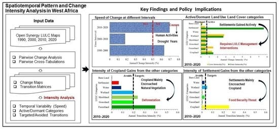
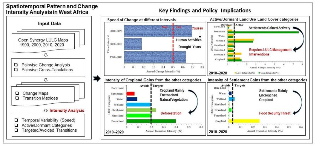
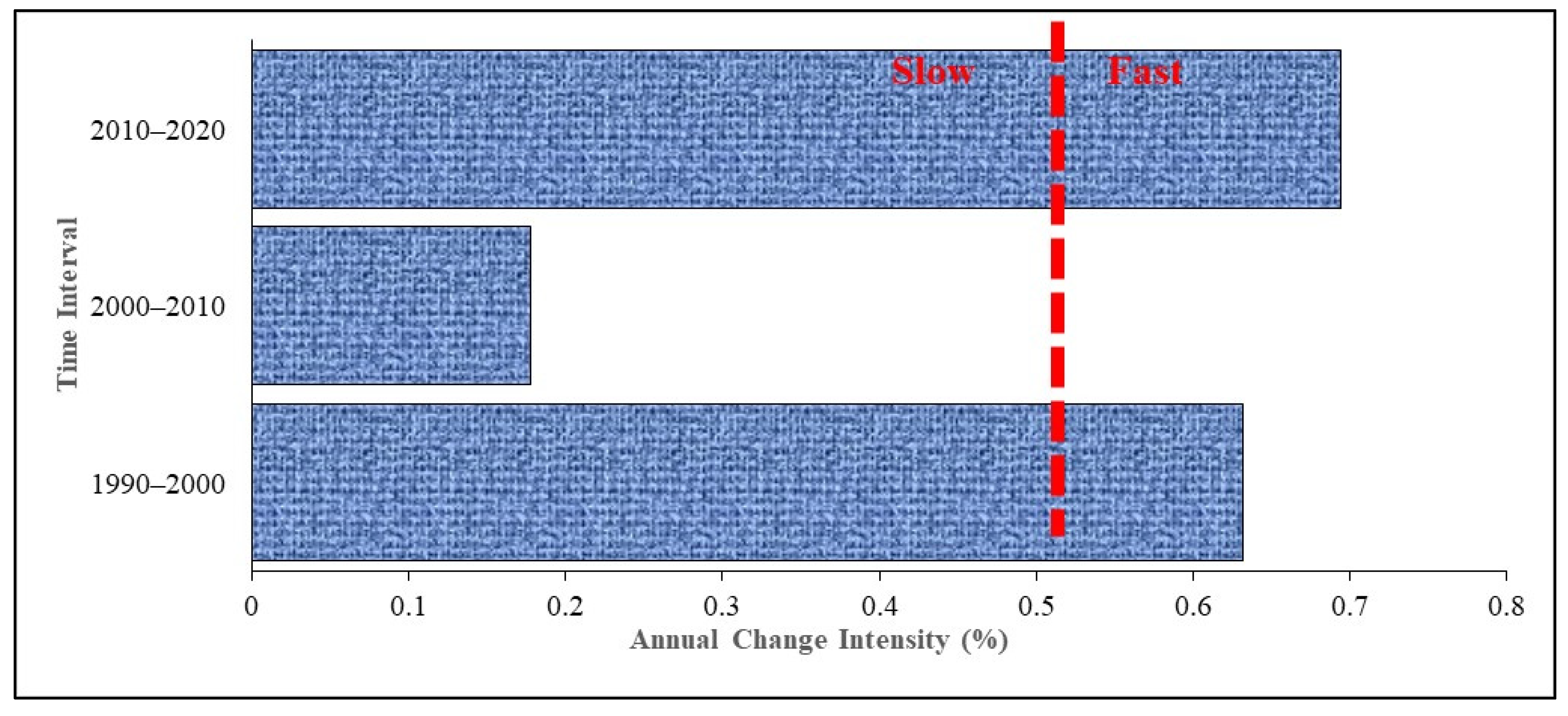
Identify the time intervals with the slowest and fastest annual rate of change.
(2)
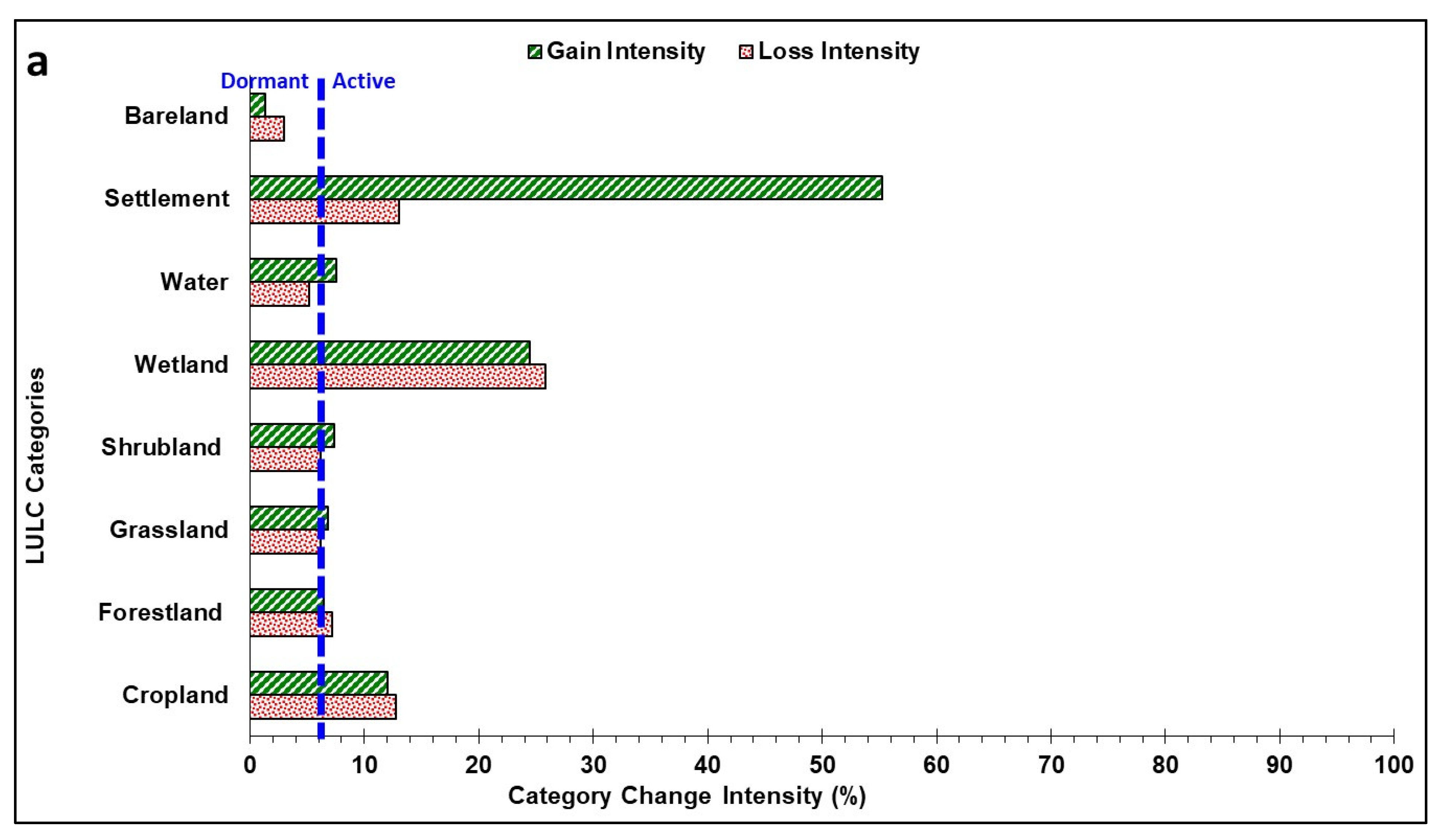
Identify the LULC categories that were relatively dormant or active in a given interval, i.e., to examine the LULC categories that gained/lost more or less than expected.
(3)
Examine the LULC categories that were avoided or targeted by a given LULC category for transition in a given interval.
We detected LULC changes in three intervals (1990–2000, 2000–2010, and 2010–2020). Further, we estimated and compared the variability of the rate of change by category and the temporal variability of gains and losses in these periods.

2. Materials and Methods

2.1. Study Area

The study was undertaken in western part of Sub-Saharan Africa. The area is located between 4° N–18° W (lower left) and 18° N–24° E (upper right) (see Figure 1). The total size of the area covered by this study was nearly 8 × 10⁶ km2, which is about a quarter of the total size of Africa. The subcontinent is characterized by five broad bioclimatic zones (Saharan, Sahelian, Sudanian, Guinean, and Guineo-Congolian) as a result of the distinctive variation in the rainfall pattern and vegetation [43].The research article by Asenso Barnieh et al. [23] gives a comprehensive account of the study area (West Africa).

2.2. Datasets

The LULC datasets were produced by Zhao et al. [44] of Tsinghua University and some of the authors of the current manuscript. To produce the datasets, we developed and applied an open and synergistic framework to combine multiple thematic LULC datasets (e.g., European Space Agency Climate Change Initiative (ESA_CCI) [45], Finer Resolution Observation and Monitoring of Global Land Cover (FROM_GLC)) [41], and other EO LULC data available in the Google Earth Engine (GEE) cloud computing platform). The open and synergistic framework combines information from supervised land cover classifications of finer resolution satellite imagery and LULC information aggregated from existing multiple thematic LULC maps and other LULC information from the GEE cloud computing platform. Here, the 30 m Landsat surface reflectance dataset, the Shuttle Radar Topography Mission (SRTM), Digital Elevation Model (DEM), ESA-CCI land cover maps, and three recent single-type land cover datasets (Global Artificial Impervious Area (GAIA) [46], GLAD Forest [47], JRC Global Surface Water (JRC_GSW) [48]) were the main input datasets for the supervised LULC classification.
The outputs were nine major land cover types, i.e., cropland, forestland, shrubland, grassland water, wetland, tundra, impervious surface, and bare land (See Figure 1). The major algorithm for the classification of these datasets was the Random Forest Classifier, the use of which was followed by an estimation of class probabilities. Cross-validation of samples was undertaken to measure the accuracy of the classification. The dataset was further improved by applying a spatial–temporal consistency model known as “Markov a Posterior Random Fields (MAP-MRF”). The overall accuracy of the maps was about 75% [44].
The temporal coverage of the final dataset from 1990 to 2020 covered the whole globe. The datasets from 2011 to 2020 can be obtained from the GEE platform by using the image collection snippet; projects/ee-fgp-annual-4/assets/fgp-annual30_2011–2020. The datasets from the year 1990 to 2020 covering only the Sahel–Sudano–Guinean region in Africa (0° and 30° N) are available at https://doi.org/10.11888/Terre.tpdc.272021 (accessed on August 2021). The analysis in this paper is restricted to the western part of Africa (4° N–18° N and 18° W–24° E) to make the results comparable to the LULC transitions analysis in our previous study [23]. The datasets were generated at five-year intervals. The analysis in this paper was conducted at ten-year (decade) intervals to minimize spurious changes and the inter-annual variability that may be introduced by residual noise in the input time series. The subsequent sections of this paper and the article by Zhao et al. [44] give details of the entire process for the development of the LULC data.

2.3. Re-Classification of the Multi-Source Land Use/Land Cover (LULC) Data

To develop the long-term historical LULC dataset, the open synergistic framework with improved validation procedure was applied to fuse LULC information from the supervised land cover classification of historical Landsat imagery, other finer resolution satellite imagery in GEE, and the reclassification of the existing LULC data in Africa [44]. The exiting LULC data were acquired from multi-sources, i.e., ESA-CCI-LULC [45], FROM_GLC [41], and single-cover LULC maps, e.g., forest cover [47], Global Artificial Impervious Area (GAIA) [46], and JRC Global Surface Water [48]. The open synergistic framework has three major steps, namely, LULC change detection with the exiting LULC maps to detect disagreement in the data for quality improvement, new LULC classification with historical Landsat archives and other finer resolutions EO data in GEE, and finally, fusion of the information from the existing LULC maps and classified Landsat imagery by data aggregation and mosaicking [44].

2.3.1. Land Use/Land Cover Change Detection

We compared the spatial locations of the existing LULC data to detect disagreement in terms of spatial locations, which is an indication of possible errors in the multi-source LULC data. The major input data for this analysis were the ESA_CCI LULC maps [45]. The seventeen classes of ESA_CCI LULC maps were aggregated into only nine LULC types, i.e., cropland, forestland, shrubland, grassland, water, wetland, tundra, impervious surface, and bare land) by grouping similar LULC types into the same categories (see Table 1). Only eight of these LULC types, i.e., all the LULC types excluding tundra, were present within the study area (West Africa).
The rationale of the aggregation was to harmonize the classification scheme of FROM-GLC with the ESA-CCI LULC maps. A change detection algorithm was applied to two LULC map pairs in the two different sources of data for a given year. Thus, the ESA-CCI-LULC maps over 6 years (1992, 1995, 2000, 2005, 2010, and 2015) were compared with the corresponding LULC maps in the FROM-GLC LULC maps by considering two LULC maps that were adjacent in terms of years (i.e., 1992 to 1995, 1995 to 2000, 2000 to 2005, 2005 to 2010, 2010 to 2015). The LULC change locations were used as masks for the subsequent analysis. Another change detection was also conducted with the GAIA datasets over 40 years at six time intervals (1992–1995, 1995–2000, 2000–2005, 2005–2010, and 2010–2015). The change locations detected by the ESA_CCI data were combined with the LULC change locations detected by GAIA data to produce the final LULC change areas, i.e., disagreement between datasets.

2.3.2. Development of a New Land Use/ Land Cover (LULC) Classification Scheme

The LULC cover maps over 40 years at five-year intervals at 30 m spatial resolution were generated by applying parallel/distributed computing techniques and machine learning algorithms. To generate the LULC maps, training samples were created with the ecoregion’s layer of the continent to train the classifier [49]. A fish net of 10 × 10 grid size was created. The area of the 14 biomes in each grid cell was estimated. The grids were categorized into groups based on the biome with the largest fractional abundance in each grid. Based on that, 12 training regions were obtained for the entire globe. This Figure 2 is in the article published by Zhao et al. in the supplementary displayed the results for the 12 training regions, and the names of the corresponding biomes for each of the 12 training regions are also shown in Table 3 of the same article [44].
Next, the training region boundaries based on the eco-region layer [49] were used to filter the training samples. Variable percentages of the training samples were defined for different LULC types to reduce the samples and ensure they were evenly distributed in the classification regions. Here, samples in other regions were used to compensate for the LULC with less than 100 samples. This action was taken to ensure the required quantity. Input feature sets were created based on spectra, phenology, and terrain properties to delineate different LULC types. All the bands of Landsat imagery, together with Normalized Difference Vegetation Index (NDVI) and Normalized Difference Water Index (MDWI), were used to calculate the required percentage.
The Landsat observations available in each year, i.e., 1990, 1995, 2000, 2005, 2010, and 2015) and in each five-year period, i.e., 1988–1992, 1993–1997, 1998–2002, 2003–2007, 2008–2012, and 2013–2017, 2017–2020, were also calculated. We maintained the completeness of the Landsat observations by filling in the missing data gaps using percentiles of the spectra bands that were derived from the five-year periods as the training features. These analyses were performed in the GEE cloud computing platform. Next, the training set and feature sets were used to develop a Random Forest classifier by setting the number of trees at 100 to identify the LULC types (cropland, forestland, shrubland, grassland, water, wetland, tundra, impervious surface, and bare land) in the locations of the LULC changes that were detected in the ESA-CCI datasets in 1990, 1995, 2000, 2005, 2010, and 2015.

2.3.3. Data Aggregation and Mosaicking

After the LULC types at the LULC change locations had been mapped, the classified maps, the FROM_GLC 2017 LULC map and the single-type LULC products (i.e., forestland, urban, and water bodies, respectively) for four periods were mosaicked to produce the open synergistic LULC Maps at five-year intervals. This procedure ensured the spatial and temporal consistency of the land cover types. The outputs were nine major land cover types (i.e., cropland, forestland, shrubland, grassland, water, wetland, tundra, urban areas/settlement, and bare land) for the entire globe and only eight LULC types in the West Africa sub-continent. The synergistic framework improved the accuracy of the LULC maps by eliminating differences due to misclassification of the individual LULC datasets from multiple sources.

2.4. Validation of the Land Use/Land Cover Datasets

The validation samples described by Li [50] were used to assess the accuracy of the LULC datasets. The results from the accuracy assessments of the six maps were around 75%, and the accuracy for change area detection was over 70%. Details of the accuracy assessment of the 2015 map can be seen in the work of Zhao et al. [44].
We assessed the consistencies of the final datasets we used for the analysis, which covered only the extent of West Africa (herein referred to as WAv2–30 m) with the two major global LULC datasets we used as input data for the synergistic data development, i.e., ESA-CCI-LC [44] and FROM-GLC_250 m [41]. We compared the statistics of the spatial distributions of cropland and forestland areas of the aforementioned datasets against the Food and Agriculture Organization (FAO)’s national level LULC statistics available at: http://www.fao.org/faostat/en/#data/RL (accessed on 6 December 2017). The LULC maps in the year 2000 were used for this comparison. We estimated the root mean squared error (RMSE) of cropland and forestland areas from each dataset against the national level cropland and forestland statistics provided by the FAO available at: http://www.fao.org/faostat/en/#data/RL (accessed on 6 December 2017).
When the national level forestland and cropland estimates of the FAOSTATS were merged into a single reference data, the relative RMSE estimates were 112.4%, 70.25%, and 54.8% for ESA-CCI-LC, FROM-GLC_250 m and WAv2–30 m, respectively. This suggests that the LULC datasets we generated from the opened synergistic approach have better agreement with the FAOSTATS. In some cases, the FAOSTATS are also limited in terms of completeness of the national statistics available at: http://www.fao.org/faostat/en/#data/R (accessed on 6 December 2017). This may partly explain the large relative RMSE we obtained for the LULC data.

2.5. Development of a Transition Matrix

The WAv2 LULC maps from 1990 to 2020 were analyzed for changes in different time intervals, i.e., 1990–2000, 2000–2010, and 2010–2020. The LULC maps in each year pair were cross-tabulated to generate a transition matrix (see Table 2). These matrices had eight LULC categories each, i.e., cropland, forestland, shrubland, grassland, water, wetland, settlement, and bare land). The sizes and intensities of changes in these LULC categories were analyzed in terms of interval, category, and transitions, following the intensity analysis framework proposed by Aldwaik and Pontius Jr. [10]. We divided each entry in the transition matrices by the extent of the study area to obtain the fractional abundance of each transition to facilitate the estimation of the uniform change intensities. This conversion was applied to changes in each time interval, specifically, 1990–2000, 2000–2010, 2010–2020) in the case of this study.

2.6. The Intensity Analysis Framework

The analyses were based on the mathematical notations and equations developed by Aldwaik and Pontius Jr. [9,18] in an Excel spreadsheet, which can be obtained for free from www.clarku.edu/∼rpontius, along with the transition matrices we generated (see Table 2). The mathematical notations and equations are listed in Table A2 in the Appendix A and Table 3, respectively. We conducted the intensity analysis at three levels (intensity, categories, and transition).
Table 3. Mathematical equations for the intensity analysis [10,16].
EquationsNo.
S t = a r e a   o f   c h a n g e   d u r i n g   i n t e r v a l   Y t ,   Y t + 1 a r e a a o f   s t u d y   r e g i o n d u r a t i o n   o f   i n t e r v a l Y t ,   Y t + 1   × 100 %   = j = 1 J i = 1 J C t i j C t j j j = 1 J i = 1 J C t i j Y t + 1 Y t × 100 %   (1)
U = a r e a   o f   c h a n g e   d u r i n g   a l l   i n t e r v a l s   a r e a   o f   s t u d y   r e g i o n   d u r a t i o n   o f   a l l   i n t e r v a l s   × 100 % = t = 1 T 1 j = 1 J i = 1 J C t i j C t j j j = 1 J i = 1 J C t i j Y T Y 1 × 100 %       (2)
G t j =   a r e a   o f   g r o s s   g a i n   o f   c a t e g o r y   j   d u r i n g Y t ,   Y t + 1   d u r a t i o n   o f Y t ,   Y t + 1   a r e a   o f   c a t e g o r y   j   a t   t i m e     Y t + 1 × 100 % = i = 1 J C t i j C t j j Y t + 1 Y t i = 1 J C t i j × 100 %                           (3)
L t i =   a r e a   o f   g r o s s   l o s s   o f   c a t e g o r y   i   d u r i n g Y t ,   Y t + 1   d u r a t i o n   o f Y t ,   Y t + 1   a r e a   o f   c a t e g o r y   i   a t   Y t × 100 = j = 1 J C t i j C t i i Y t + 1 Y t j = 1 J C t i j × 100 (4)
R t i n = a r e a   o f   t r a n s i t i o n   f r o m   i   t o   n   d u r i n g   Y t , Y t + 1 d u r a t i o n   o f Y t , Y t + 1   a r e a   o f c a t e g o r y   i   a t   t i m e   Y t × 100   = C t i n Y t + 1 Y t j = 1 J C t i j × 100     (5)
W t n = a r e a   o f   g r o s s   g a i n   o f   c a t e g o r y   n   d u r i n g   Y t ,   Y t + 1 d u r a t i o n   o f   Y t ,   Y t + 1 a r e a   t h a t   i s   n o t   c a t e g o r y   n   a t   t i m e   Y t × 100 %   = i = 1 J C t i n C t n n Y t + 1 Y t j = 1 J i = 1 J C t i j C t n j × 100 %               (6)
Q t m j =   a r e a   o f   t r a n s i t i o n   f r o m   m   t o   j   d u r i n g Y t ,   Y t + 1   d u r a t i o n   o f Y t ,   Y t + 1   a r e a   o f   c a t e g o r y   j   a t   t i m e   Y t + 1 × 100 %   = C t m j Y t + 1 Y t i = 1 J C t i j × 100 %         (7)
V t m = a r e a   o f   g r o s s   l o s s   o f   c a t e g o r y   m d u r i n g   Y t ,   Y t + 1 d u r a t i o n   o f   Y t ,   Y t + 1 a r e a   t h a t   i s   n o t   c a t e g o r y   m   a t   t i m e   Y t + 1 × 100 %           = j = 1 J C t m j C t m m Y t + 1 Y t i = 1 J j = 1 J C t i j C t i m × 100 % (8)
M t i j = a r e a   o f   t r a n s i t i o n   f r o m   i   t o   j   d u r i n g   Y t , Y t + 1   a r e a   o f   c a t e g o r y   i   a t   t i m e   Y t = C t i j j = 1 J C t i j     (9)
Firstly, we calculated the change intensity for each interval and compared the observed rate with the uniform rate that would have occurred if the annual changes were distributed uniformly across the entire time extent. We then identified the time intervals with the slowest and fastest annual rate of change. Secondly, we calculated the intensity of gross losses and gains for each category and compared the results, i.e., the observed change intensities with a uniform intensity of annual change that would occur if the changes within each interval were distributed uniformly over the entire spatial extent. The LULC categories that were relatively dormant or active were identified. Thirdly, we calculated the observed intensity of each transition and compared the observed intensity of each transition with a uniform intensity among the categories available for those transitions. The categories that were avoided or targeted by a given category for a transition were identified. We indicated a transition of a category as random when the rate of change was proportional to the initial abundance of a category and systematic when it specifically targeted or avoided a particular category for a transition [10]. Detailed intensity analysis at three levels are explained below.

2.6.1. Identification of the Time Intervals with the Slowest and Fastest Annual Rate of Change

To understand the variation in the intensity of change in different time intervals, the annual rate of change on the landscape was estimated for each time interval by applying Equation (1) in Table 3. This facilitated a comparison of changes in different periods of time, as proposed by Runfola and Pontius Jr. [51]. Equation (1) takes into account the duration of each interval to give one rate of change per time interval at each level of spatial aggregation. The results from Equation (1) for each time interval were compared with a constant annual rate (uniform change intensity) estimated for all the time intervals combined, i.e., from the initial time point to the final time point of the entire analysis by applying Equation (2). Equation (2) yields one uniform rate for the entire temporal extent of the study. If S t   in Equation (1) remains unchanged for the entire temporal coverage, S t will be equal to U in Equation (2), which is the uniform annual rate. According to Aldwaik and Pontius Jr. [10], this logic holds true for the analysis of all the other levels of intensity analysis. The annual rate of change for a given interval is considered slow if it is lower than the uniform rate and fast when higher than the uniform annual rate U obtained by Equation (2).

2.6.2. Identification of the Land Use/Land Cover (LULC) Categories That Were Relatively Dormant or Active

The intensities of annual gross losses and gains in each category at each time interval were analyzed to understand how the magnitudes of loss and gain intensities varied across space and time. These were calculated for each category in each time interval by applying Equations (3) and (4), respectively, and the outputs were compared with the uniform intensity of annual change in each time interval (t), i.e., the value obtained by applying Equation (1). This information was crucial to understanding which category was relatively dormant or active in a given interval. Here, there is a linkage between the interval and category level analysis. In Equations (1) and (3), G t j   =   S t when equal gains are obtained for all the   j . Similarly, in Equations (1) and (4), L t i   =   S t when equal losses are obtained for all   t h e   i . Annual loss or gain intensity below the estimated uniform change intensity for a given category indicates a relatively dormant category. Likewise, annual loss or gain intensity above the estimated uniform change intensity for a given category indicates a relatively active category. This analysis was essential to detect stable patterns in the annual loss and gain intensity for each category.

2.6.3. Examination of the Land Use/Land Cover (LULC) Categories That Were Avoided or Targeted for Transitions

To determine which transition was relatively intensive in a given interval, each transition, e.g., forestland transition to cropland, was analyzed to understand the variation in magnitude and intensity. The patterns of gains and losses in the categories n and m, respectively, were analyzed (see Table A2 in the Appendix A for description of notations n and m). The observed intensities of each transition were compared with the uniform intensity, i.e., the average over all transitions.
The transition intensity level of analysis yields two sets of outputs. One output is gains of category n from other categories and another is the loss of category m to other categories. Taking for instance, the pattern of gain of category n, the analysis was essential, e.g., to identify why the transition from natural vegetation to cropland was larger than the mean magnitude of cropland gains. Aldwaik and Pontius Jr. [10] attributed such transitions to the fact that the natural vegetation area at the initial time may be larger than the other categories. Hence, if cropland gain was distributed proportionally across the landscape, more natural vegetation areas may transition to cropland than to any other category. Another explanation offered by Aldwaik and Pontius Jr. [10] was that cropland gains might systematically target natural vegetation rather than the other LULC types.
Therefore, based on the estimated gross gain of category n, Equations (5) and (6) were applied to understand whether the gains in the individual categories, in particular, natural vegetation, were due to a random or systematic process. The analysis provided more information about the categories which were intensively avoided or targeted by category n for transitions in a given time interval. Based on the observed gross gain of category n, Equation (5) yields a single result for each time interval (t), that is, the uniform intensity of transitions to category n, i.e., the mean gain of category n across the landscape. The W t n   in Equation (5) will be equal to R t i n   in Equation (6) for all   i when the gains in n are distributed uniformly across the landscape, i.e., under a random process of gain. The observed intensities of the transitions from category i to category n for all non-n categories were determined by Equation (6). This yielded a single result for each category i per time interval. Here, it must be noted that category n could only gain from categories that were not n at the initial time interval. Therefore, if the gains in category n were uniform across the landscape, that means the gains in category n were proportional to the initial extent of those other categories. The transition from category m to category n is stationary if category n either targets or avoids m in all the time intervals.
The loss intensity for each category was estimated with Equations (7) and (8) based on the estimated gross loss of category m. This analysis revealed the other categories that systematically avoided or targeted losing to category m. Here, the assumption was that it was impossible for category m to lose at the location it occupied at the end of the time interval. Equation (7) yielded the uniform intensity of the transitions from category m to all other categories for a given interval. The output from Equation (8) is the intensity of the transition from category m to category j for all the non-m categories for each time interval. Q t m j = V t m for all j if the loss in category m to the other categories was uniform. The intensities in all the time intervals were examined to identify stable (stationary) transitions. Based on the losses of category m, a transition was considered stationary when category m is either avoided by category n for all the time intervals or targeted by category n for all the time intervals. The intensity analysis at the transition level presented in this section differs from Markov transition analysis, as the proportion of each LULC transition in a Markov matrix is estimated by Equation (9).

3. Results

3.1. Comparison of the Land Use/Land Cover (LULC) Maps in Different Years

The LULC maps in Figure 2 of this study are a comparison of the situations in 1990 (a), 2000 (b), 2010 (c), and 2020 (d) in West Africa (see Table A1 in the Appendix A for the full names of the countries on the map). Essentially, we observed the concurrent expansions and reductions in the LULC categories at different locations in West Africa. We observed the encroachment of settlements on cropland fields and cropland encroachment on natural vegetation areas. Despite the massive loss we observed for natural vegetation, particularly forestland, in some parts of the study area, such as in Nigeria, Cote d’Ivoire, Ghana, and Togo, there were some isolated areas in Niger, Burkina Faso, Mali, and Senegal where we detected natural vegetation regrowth. Figure 3 shows the locations of natural vegetation gains (greening/new growth) for 1990–2020 in West Africa. The subsequent sections provide more details about the extent and nature of the LULC transitions we observed in the study area.

3.2. Identification of the Time Intervals with the Slowest and Fastest Annual Rate of Change

The highest annual rate of change (0.69%) was observed in 2010–2020, followed by 1990–2000 (0.63%). The lowest annual rate of change intensity was observed in 2000–2010, i.e., 0.18%, which was below the mean annual rate change, thus indicating a slower process of change during this period (see Figure 4).

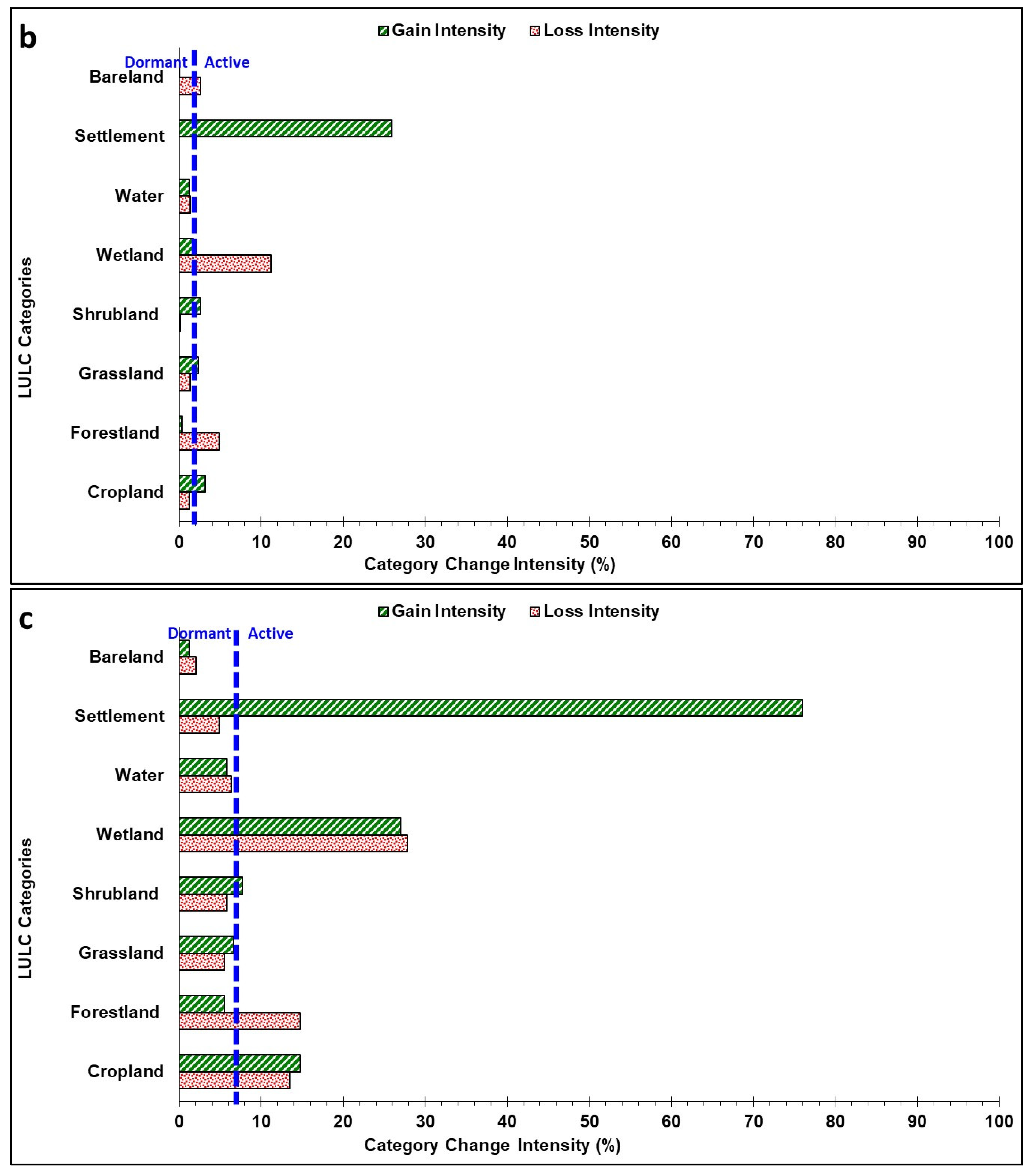
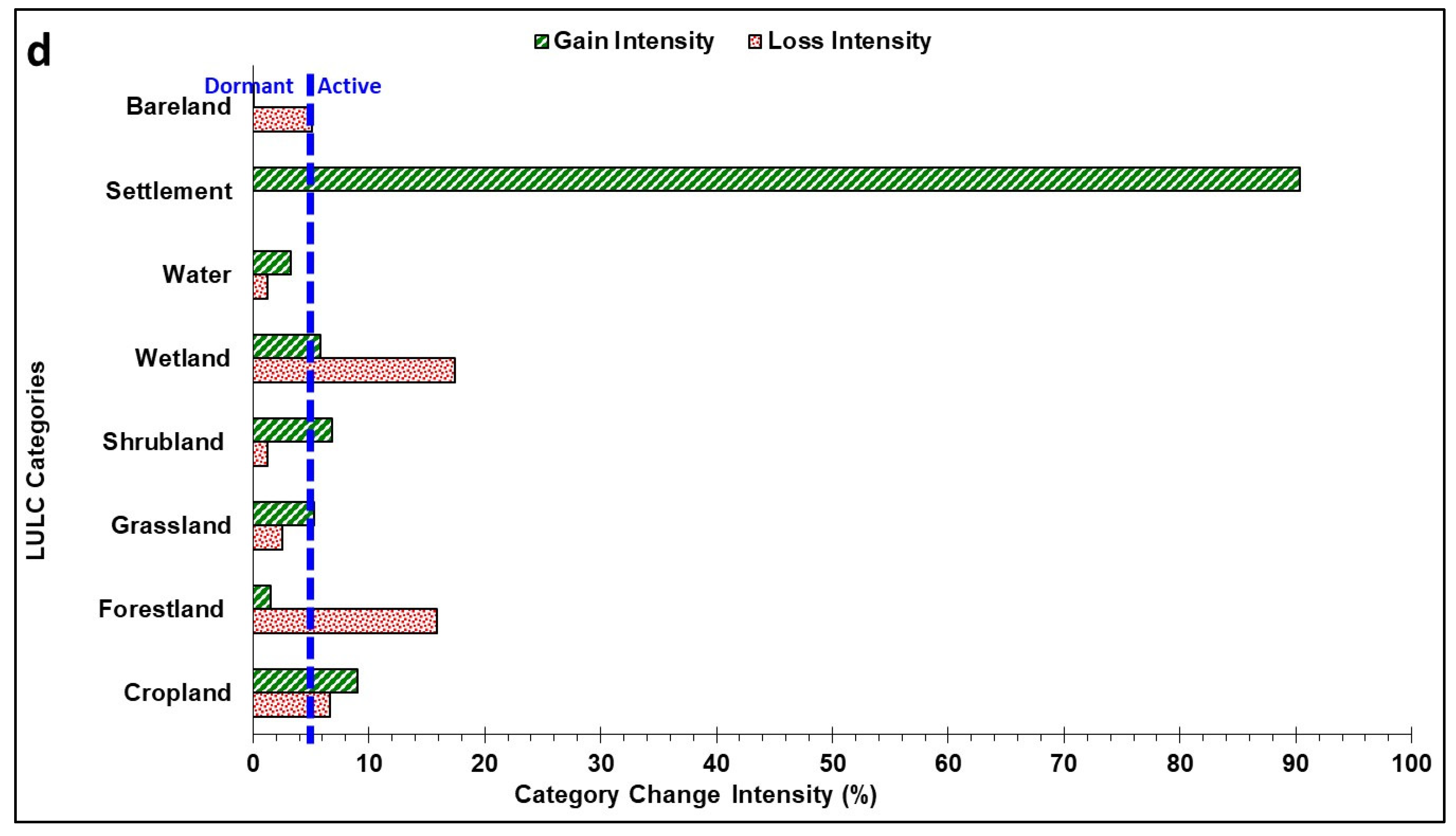
3.3. Identification of the LULC Categories That Were Relatively Dormant or Active in a Given Interval

At the category level, settlement, cropland, and wetland both actively gained and lost in 1990–2000. Water bodies actively gained in extent, while the loss intensity was dormant in the same period. During 2000–2010, cropland, grassland, shrubland, and settlement actively gained in extent. The remaining LULC were dormant in gaining, while forestland and wetlands showed some active losses. During 2010–2020, cropland, settlements, and shrubland actively gained, while wetlands actively gained in some areas and actively lost in other areas. The extent of the remaining LULC categories did not change significantly during this period, as they were dormant in gaining and losing at the same time. Settlements showed the highest annual gain intensity, i.e., 5.53%, 2.60%, and 7.60%, respectively, in 1990–2000, 2000–2010, and 2010–2020 (Figure 5 and Figure 6).
During the three periods, settlements and cropland were active gainers, whilst bare land and forestland were dormant. The gain intensities of these four LULC categories were stationary. The annual gain intensities of the remaining LULC categories were not stationary. Regarding losses, only wetlands were the active loser throughout the entire study period, i.e., stationary. All the other LULC categories were either active losers or dormant losers in one or more periods, i.e., non-stationary (see Figure 5 and Figure 6).
Figure 6 shows the loss and gain intensities of the various LULC categories every 10 years. The sum of the loss and gain intensities, with sign, of each category gives a decadal net change (%). For the entire period (1990–2020), the net change was negative (loss) for forestland, wetland, and bare land. The net change was positive (gain) for the remaining categories, i.e., cropland, settlement, shrubland, and grassland (Table 4). The net gains in rangeland (i.e., shrubland and grassland) are of paramount importance, as previous studies [23,24,25] on the continent detected consistent losses in natural vegetation categories, except for herbaceous vegetation.
We observed that almost all the categories gained and lost simultaneously (Figure 5 and Figure 6). Regarding the net change in 1990–2000, 2000–2010, and 2010–2020, forestland, bare land, wetland, and water bodies had net losses, with the exception of the net change for water bodies, which was positive in 1990–2000. Gains were identified in the net change for all the remaining LULC categories, except cropland, which had a net loss in 1990–2000. For 2000–2010, gains were recorded for cropland, grassland, shrubland, and settlements. The remaining categories, i.e., wetlands, water bodies, forestland, and bare land experienced losses. The entire period (1990–2020) saw expansion of water bodies accompanied by vegetation (shrubland, grassland) recovery (Figure 2 and Figure 3 and Table 4).

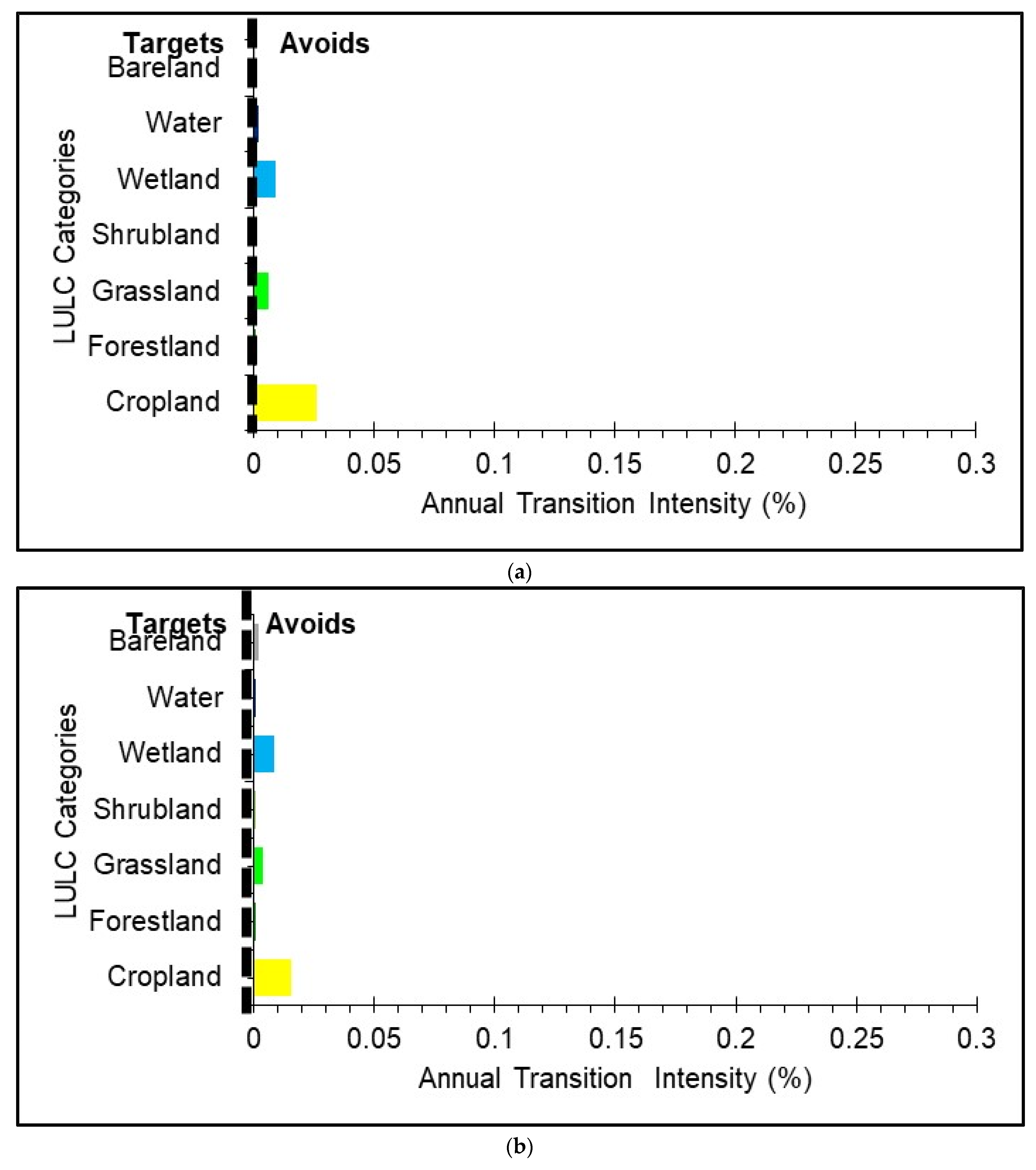
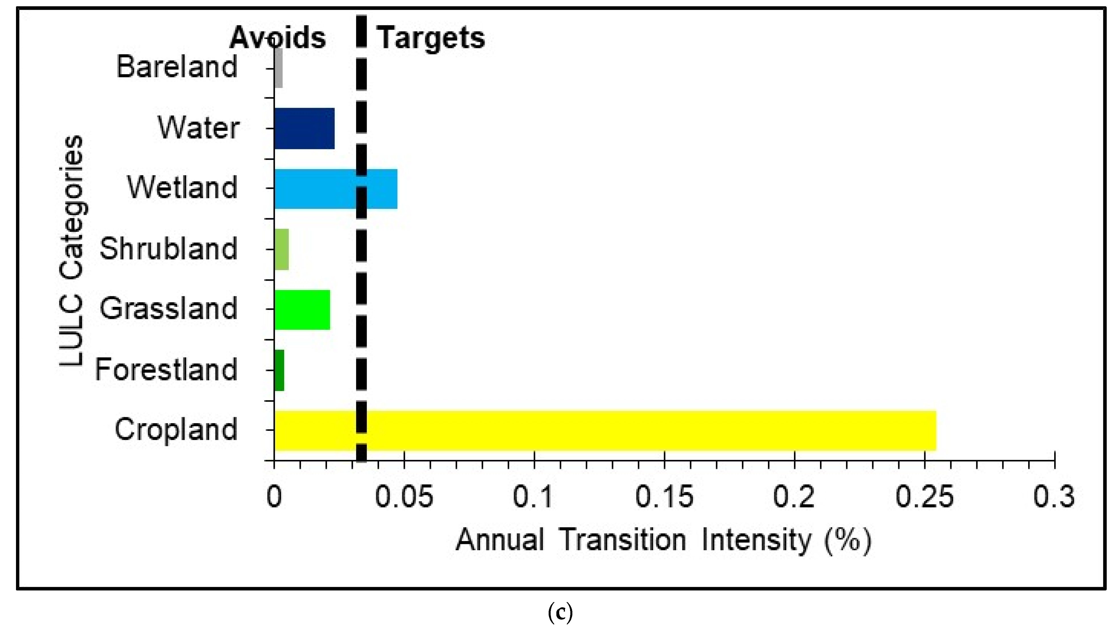
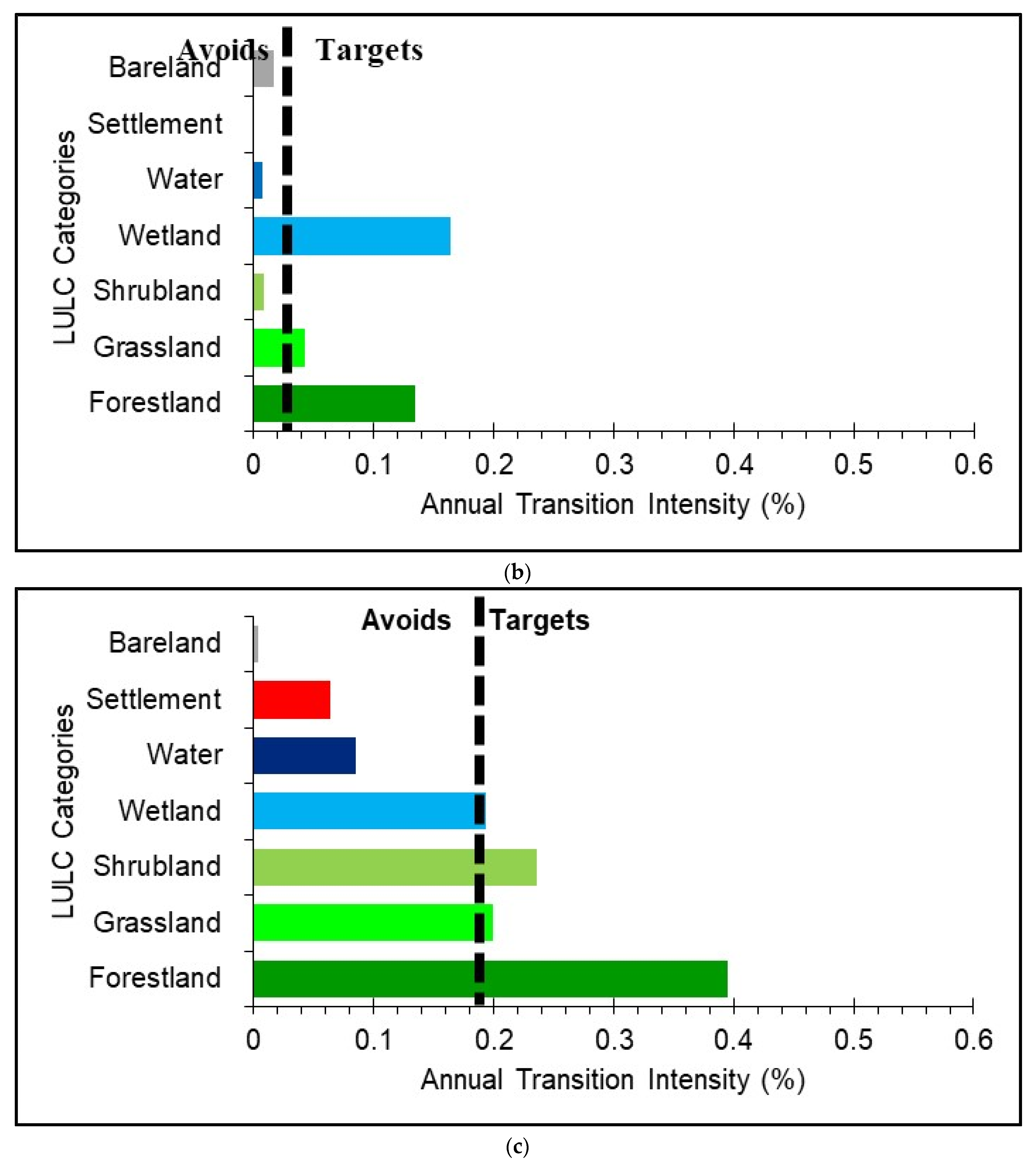
3.4. Examination of the LULC Categories That Were Avoided or Targeted for Transitions

Regarding the fractional abundances of transitions, the focus was on the gaining categories—most importantly, natural vegetation, i.e., grassland and shrubland gains from the remaining LULC categories. Previous LULC change analysis in West Africa revealed consistent losses in natural vegetation areas [23,24,25]. We also focused on settlement and cropland gains from the remaining categories, as they were active in all the three periods. Figure 7 shows the concurrent losses and gains in the LULC categories in West Africa over time. Figure 8, Figure 9, Figure 10 and Figure 11 illustrate the annual transition intensities of the major LULC categories. The annual transition intensity for each major gaining category is expressed as a percentage of the initial size of the losing category involved in the transition. Likewise, the annual transition intensity for each major losing category is expressed as a percentage of the final size of the gaining category involved in the transition. Details of the specific transitions are presented in the subsequent sections.

3.4.1. Shrubland, Grassland, Cropland, and Settlement Gains

The shrubland category targeted gaining from the cropland and forestland categories only in 1990–2000 and 2010–2020. In the former period, the annual shrubland gains from cropland and forestland were 0.64% and 0.47%, respectively. These gains were above the uniform annual transition rate of 0.27%. In 2000–2010, shrubland targeted gaining from forestland (0.27%) and wetland (0.23%). These annual rates of change were above the uniform annual rate of transition, i.e., 0.1%. In the last period, approximately 0.55% and 0.82% of the gains in shrubland were due to encroachment on cropland and forestland, respectively. The uniform transition rate for this period was 0.30% (Figure 8).
Grasslands mainly replaced wetland (0.66%), settlement (0.56%), cropland (0.46%), and bare land (0.26%) in the first period, i.e., 1990–2000. These amounts were above the uniform annual rates of transition (0.24%) for that period. In the 2000–2010 period, only wetlands (0.25%), bare land (0.22%), and water bodies (0.11%) lost to grasslands. These annual rates of change were above the uniform annual transition rate (0.08%). In the last period, i.e., 2010–2020, wetland (0.84%), cropland (0.46%), settlement (0.31%), water bodies (0.25%), and bare land (0.24%), targeted losing to grassland. The uniform annual rate of transition for this period was 0.24% (Figure 9).
Settlements gained significantly during all periods (Figure 10). In 1990–2000, these annual gains were at the expense of cropland (0.03%), grasslands (0.006%), and wetlands (0.009%). Similarly, in 2000–2010, cropland (0.015%), grassland (0.0035%), and wetlands (0.0085%) were targeted for transitions by the settlement category. The remaining categories were avoided for transitions by the settlement category. In 2010–2020, settlement targeting gaining from cropland (0.25%) and wetland (0.05%) only. The uniform annual transition rates were 0.005%, 0.0032%, and 0.04% for 1990–2000, 2000–2010, and 2010–2020, respectively (Figure 10).
During the 1990–2000 period, in West Africa, cropland targeted gaining from grassland (0.21%), shrubland (0.21%), wetland (0.20%), and settlement (0.05%) categories annually. The remaining LULC categories were avoided for replacement by cropland. In the 2000–2010 period, the annual gains in cropland were mainly at the expense of wetland (0.16%), forestland (0.13%), and grassland (0.04%). In the 2010–2020 period, shrubland (0.24%) was also targeted for transitions in addition to grassland (0.2%), wetland (0.193%), and forestland (0.04%). The uniform annual transition rates were 0.15%, 0.04%, and 0.19% for 1990–2000, 2000–2010, and 2010–2020, respectively (Figure 11).

3.4.2. Forestland, Wetland, Water Bodies, and Bare Land Losses

Overall, from 1990–2000, the losses in forestland were mainly due to encroachment by wetland (0.76%), shrubland (0.23%), water bodies (0.18%), settlements (0.18%), and cropland (0.15%). In the 2000–2010 period, forestland targeted losing to cropland (0.16%), shrubland (0.13%), and settlements (0.11%), against a uniform rate of transition of about 0.08%. In the 2010–2020 period, forestland was targeted for encroachment by wetland (0.69%), cropland (0.44%), and shrubland (0.37%).
In the 1990–2000 period, wetlands targeted losing to water bodies (0.09%), settlements (0.005%), and forestland (0.002%). In the 2000–2010 period, wetlands targeting losing to water bodies (0.007%), settlement (0.003%), forestland (0.0015%), and cropland (0.0007%). In the 2010–2020 period, wetlands lost to water bodies (0.08%), settlement (0.004%), forestland (0. 003%), and grassland (0.001%).
Likewise, in the 1990–2000 period, water bodies targeted losing to settlements (0.1%), wetland (0.062%), forestland (0.01%), cropland (0.0035%), and grassland (0.00313%), with a uniform annual rate of transition of about 0.0023%. However, from 2000 to 2010, only the wetlands (0.04%), grassland (0.002), and settlement categories (0.0012%) targeted water bodies for transitions. These annual transition rates were above the uniform annual transition rates of 0.00063%. In the 2020–2020 period, water bodies targeted losing to wetlands (1.064%), settlements (0.021%), forestland (0.0063%), grassland (0.0043%), and cropland (0.0034%). These annual transition rates were above the uniform annual transition rate (0.0029%).
In the case of bare land, losses were mainly due to encroachment by the grassland and settlement categories. The annual transition rates of bare land to settlements were (0.27%), (0.36%), and (0.15%) in 1990–2000, 2000–2010, and 2010–2020, respectively. In the same periods, the annual transition rates of bare land to grassland were 0.27%, 0.18%, and 0.16%, respectively, which were higher than the uniform annual rates of transitions, i.e., 0.09%, 0.07%, and 0.06%, respectively.

4. Discussion

4.1. Identification of the Time Intervals with the Slowest and Fastest Annual Rate of Change

The study took into account the duration of the different time intervals and examined the sizes and intensities of LULC change to carry out a detailed analysis of the stationarity of the observed transitions. At the interval level, we detected a faster annual rate of total change in the period of 1990–2000 and 2010–2020. We attributed our findings to the combination of severe drought and human activities, e.g., the expansion of artificial water bodies to meet irrigational requirements. We observed gains in the area covered by water bodies despite the preceding drought years and the massive concurrent expansion of settlements in parallel with croplands in the most recent period (2010–2020).
The concurrent losses and gains of the LULC categories we detected at the category level of our analysis may also explain the reason why we detected a faster annual rate of total change in the period of 1990–2000 and 2010–2020 at the interval level in West Africa. Thus, a deeper analysis at the category level revealed more changes in the periods of 1990–2000 and 2010–2020, i.e., we observed both active losing and gaining intensities for categories thought to be dormant losers and active gainers. For example, in reality, the category of settlement is a dormant loser, active gainer, and a persistence category in different periods. However, here we observed that, in different regions, the settlement category was both an active gainer and loser during the 1990–2000 period, i.e., soon after the severe drought spells. The category of settlement losing actively in the aforementioned periods could be linked with possible errors in the datasets, as the accuracy of the LULC data we used for the analysis was not 100%. The overall accuracy of the LULC datasets was about 75% [44].
We attributed these findings to the fact that farmers in West Africa’s rural areas live very close to farmlands, forestland, and other vegetation areas. It is common to mix up the RS mapping of small thatch settlements, croplands, forestsland, and other vegetation [52]. Therefore, the deviation of the settlement loss from the uniform intensity might be partly due to systematic errors in the LULC datasets.
This confirms the explanation by Aldwaik and Pontius Jr. (2013) [16] that errors in the LULC categories may influence the results from the transition analysis. The results from this analysis are in agreement with the LULC analysis we conducted with the USGS LULC maps at three time periods (1975–2000, 2000–2013, and 1975–2013; Subfigures (ac)) in West Africa [53]. In the aforementioned previous study [53], we observed a larger categorical exchange between the LULC categories in the drought period (1975–2000) than in the period between 2000 and 2013.

4.2. Identification of the LULC Categories That Were Relatively Dormant or Active in a Given Interval

The results revealed that the settlement, cropland, forestland, and wetland categories are the major active categories. At the initial stage (1990) of the LULC transition (1990–2000 and 2000–2010, 2010–2020) analyses, shrubland and grassland constituted a greater proportion of the total land area in the study area. Therefore, if changes were distributed uniformly across the landscape, shrubland and grassland were expected to lose more than any other category. Nevertheless, the intensity analysis revealed that in 1990–2000, shrubland and grassland categories in some regions were dormant losers, and in other regions, they were active gainers. In the 2000–2010 period, two categories (shrubland and grassland) were slightly active gainers and dormant losers in different periods. In the later interval (2010–2020), grassland was a dormant loser and gainer, whilst shrubland was a dormant loser and a slightly active gainer. Here, the dormancy of grassland and shrubland may be due to their large persistence, which was included in the intensity analysis [10].
The influence of the large dormant categories, such as grassland and shrubland in the case of this study, on the intensity of the transitions has been underlined by Aldwaik and Pontius Jr. (2012) [10] and Quan et al. (2019) [17]. According to Aldwaik and Pontius Jr. (2012) [10] and Quan et al. (2019), if, for instance, grassland accounts for a larger proportion of the landscape and does not change over time, then its presence in the analysis implies that all the other non-grassland categories will be active than normal [17]. This may indicate that losses or gains in a category that is at the final stage of a transition could be explained by its largest size at the initial stage and whether the category avoided transition from the remaining categories or whether it was targeted for a transition. According to Aldwaik and Pontius Jr. (2012) [10], in some instances, a large dormant category plays a minimal role in the total change. A typical example is water body. However, then it is crucial to include water bodies in LULC change analysis in a setting where “humans convert water to land via infill or convert land to water via dams,” which is the case in this study area (West Africa) [14].
Aldwaik and Pontius Jr. (2012) [10] recommended that, to minimize the influence of a large dormant category on the intensity analysis, categories which bring a large persistence into the analysis must be eliminated. Shrubland and grassland dormancy in losses may be explained by positive human activities and interventions, such as the farmer-led natural regeneration initiative and the great green wall policy in West Africa [54]. In addition, we detected transitions of cropland fields into grassland and shrubland, which may also indicate the abandonment of some cropland fields in West Africa [55]—triggered by the declining food prices and migration of farmers [56]. Though we observed net gains in cropland fields in the middle and last periods (2000–2010 and 2010–2020), this category was involved in large exchange, i.e., both the gross losses and gains were active during the first and last periods (1990–2000 and 2010–2020). The exchange between cropland and the remaining LULC categories meant that net change for this category was negative (net loss) in the first period (1990–2000). The current finding is an exception because net gains have been consistently observed in the cropland category by all the previous LULC change analysis conducted over the continent at all the temporal periods of analysis [23,24,25]. The simultaneous active gross loss and gain intensities of cropland fields in the 2010–2020 period (later period) raise food security concerns and should act as an early warning sign to policy makers that the food security of some marginal geographic locations is under threat despite the massive expansion of cropland observed in this area.
The net gains in the categories of shrubland, grassland, and water bodies during the 1990–2020 period confirm the long-contested re-greening in West Africa [54,57,58]. By contrast, previous LULC analyses on the continent revealed net losses in the other vegetation categories, i.e., shrubland and grassland, in the case of this study [23,24,25]. The differences in temporal resolutions of the LULC datasets we used for this study and our previous analysis might have accounted for the contrasting results.
Regarding the stationarity of the categories, the pattern of gains in the settlement category was consistent throughout the intervals, i.e., the settlement category demonstrated stationarity in actively gaining, whilst the remaining LULC categories exhibited un-stationarity. We attributed this finding to population growth and the quest for urban expansion on the continent [59].

4.3. Examination of the LULC Categories That Were Avoided or Targeted for Transitions

The analyses of the entire transition processes gave a clearer view of the development that led to the massive expansion of cropland in the second and last periods (2000–2010 and 2010–2020), as we observed the replacement of shrubland and grassland by cropland. Comprehensive analysis at the transition level revealed that cropland systematically targeted shrubland, grassland, forestland, and wetlands for transitions. This may be attributed to the high nutrient values of natural vegetation and wetlands sites to support crop growth. It may also indicate that the spatial dependence of a given category affects how it tends to replace any neighboring category on the landscape [14]. Therefore, Pontius Jr. (2019) [14] suggested a visual examination of the maps to confirm the influence of spatial dependence on transitions among categories. In the case of this study, visual examination of the LULC maps and field analysis suggest that farmers live in close proximity to natural vegetation, e.g., forestland and other vegetation (shrubland, grassland, etc.) areas. Hence, the likelihood of natural vegetation transitions to cropland may increase.
Concurrently, the settlement category mainly targeted cropland for transitions. Cropland replacement by settlements was one of the most pronounced observed systematic transitions on the landscape due in part to the easiness of conversion, i.e., less labor and lower costs involved. In addition, farmers prefer to change unproductive cropland to settlement rather than to transform productive natural vegetation field, which could be used for productive farming, into settlements. Huang et al. (2018) [15] also found a large and systematic transition from cropland to settlements which, according to them, visual examination of the patterns in the maps revealed outward expansion of settlement patches to encroach cropland. In the case of settlement replacing forestland, this may be associated with the fact that urbanization in West Africa is more localized in the forest-rich humid areas and, as explained by Pontius Jr. (2019) [14] and evidenced by Huang et al. (2018) [15], the fact that LULC categories may target the closest neighboring cells for replacement. Cropland targeted natural vegetation for transitions and settlements targeted cropland, which confirms the assertion that urbanization threatens cropland fields.
We observed forestland replacement by shrubland and cropland, which indicates land degradation and deforestation, respectively. In the forest-rich areas, this may be attributed to the rapid rise in population and economic growth, as well as the quest to fulfil the food security of the people. Simultaneously, we observed isolated gains in the area covered by forestland during the 1990–2020 period. Some areas previously covered by shrubland were consistently replaced by forestland at all of the temporal scales (1990–2000, 2000–2010, and 2010–2020). This might have been due in part to the implementation of Land Use Management policies such as the farmer-managed natural resources rehabilitation program, which involved the replanting of trees on degraded landscapes [54].
Though the use of the intensity analysis framework we employed for this analysis (see Section 2.6) has not been fully explored to link patterns with processes with regard to the African landscape, the results from this analysis are consistent with other LULC change analyses on the continent [23,24,25]. Many results of these other analyses suggest that human-induced LULC change is accelerating over time as they were all active gainers [23,24,25]. The sizes of the LULC transitions can be seen in the traditional Markov transition matrix. However, deeper examination is required to link patterns with processes as intensity analysis probes the transition matrix to reveal the matrix’s detailed patterns [14].
The influence of class aggregation on the analysis, particularly regarding the development of the LULC maps, must be given careful consideration, as seventeen LULC types were aggregated into only nine LULC classes [23]. The analysis of the original LULC types may have been sensitive to the aggregation of the category.

5. Conclusions

This study bridged the LULC data gaps by fusing useful information from existing multi-source LULC data with information from very high-resolution data from the GEE cloud computing platform. This reduced the discrepancies in the LULC datasets and improved their accuracy. This study is the first attempt to use long-term and up-to-date finer resolution (30 m) LULC data in a synergistic approach for LULC change analysis in West Africa. We analyzed the spatial patterns and processes in LULC categories on the landscape of West Africa by using historical LULC data and a unified intensity analysis framework that worked on three levels: interval, category, and transition. We detected faster annual rates of transition, 0.63% and 0.69%, respectively, for the 1990–2000 and 2010–2020 periods, and attributed these faster rates to the severe drought of the 1970s and the 1980s, in the case of the former, and intensive human activities in recent years, in the case of the latter. Similar to our previous LULC transition analysis on the sub-continent, we found simultaneous losses and gains in the LULC categories, which indicate the spatial reallocation of the categories. In the case of cropland, both the active losses and gains are a cause of policy concern as the massive gains threaten the conservation of natural vegetation, whilst the losses as a result of encroachment by the settlement category may threaten the food security of the growing and vulnerable population.
The analysis at the transition level highlighted the dormancy of shrubland and grassland in losing despite being targeted for transition by actively gaining categories such as cropland. The introduction of some LULC change management policies (REDD+, Farmer Managed Natural Regenerative Initiative, and so forth) in the sub-continent might have slowed down the loss of rangeland (shrubland and grassland). The net gains in shrubland and grassland (re-greening) were due in part to replanting and, on the other hand, degradation of forestland as we observed the massive replacement of forestland by shrubland and grassland. We also observed encroachment of the settlement, cropland, water bodies, and wetland categories on forestland, which indicate deforestation. Deforestation is often associated with fires that release large amounts of carbon dioxide (CO2) into the atmosphere, potentially further hindering climate change mitigation on the continent. Additional effort is therefore required to curb forest degradation and deforestation on the sub-continent despite the relative gains of rangeland we observed on this landscape. Geo-spatial land planning and buffer zones are urgently needed to protect pristine forest and other natural resources on the continent.
The results suggest that the LULC transitions in West Africa were not only due to the larger fractional abundance of some categories at the beginning of the transition but also due to systematic targeting by actively gaining LULC categories such as settlements, e.g., the net relative gains in settlements were 48.57%, 25.96%, and 74.75 % in the periods of 1990–2000, 2000–2010, and 2010–2020, respectively, and 90.39% in 1990–2020. Our results indicate that LULC changes on the landscape of West Africa are both systematic, i.e., under the influence of humans, and random, i.e., driven by natural factors depending on the type of transition. The study highlights important signals in the pattern of the LULC transitions and may serve as a foundation to link the observed pattern with explanatory variables to understand the processes underlying the intensive gains of settlements. The current transitions may greatly affect biodiversity, carbon stock enhancement, and the food security of the people. Agroforestry, community-led land rejuvenation activities, alternative livelihoods, and diversification of income may present good opportunities to protect the environment and reduce the susceptibility of the human system to shock.
The study also improved our understanding of the active and dormant LULC categories in the study area and revealed the LULC categories that were avoided or targeted for transition in a given interval. The intensity analysis provided a basis to focus LULC management interventions toward the actively changing categories, e.g., the expansion of settlements, instead of focusing on entire dynamic processes that may be cost-intensive. This study is the first to use LULC change analysis to document consistent net relative gains (re-greening) in rangeland in West Africa from 1990 to 2020 in order to support the re-greening hypotheses present in the literature. Future research must analyze the impact of LULC change on food security and water balance. The opportunity cost of maintaining cropland (e.g., cash crops) and compliance with LULC change management interventions must also be analyzed.

6. Policy Recommendations

This research recorded concurrent deforestation and vegetation regrowth in different locations in West Africa. These findings were attributed to human activities, such as the uncontrolled expansion in settlements and cropland at the expense of natural vegetation areas, and positive human activities, such as the implementation of nature-based solutions and land degradation restoration projects, respectively, on the subcontinent. The results indicate that the sustainable management of forests, good farming practices, and community involvement can help to minimize deforestation and recover degraded land in West Africa. Therefore, we recommend that the implementation of nature-based solutions, such as the farmer-led Natural Regeneration of Trees and Resilience Building Strategies, Great Green Wall Initiatives, Agroforestry practices, and REDD+ policies, must be up-scaled across the Africa continent. We detected simultaneous losses and gains in cropland fields, which raise food security concerns in West Africa. Based on our findings, we recommend the implementation of sustainable agricultural practices, such as effective soil management, e.g., application of cow dung and organic manure to restore soil fertility, cultivation of climate-smart and drought-resistant crops, and alternative sources of livelihood for the farmers. The agriculture value chain in Africa must be strengthened.
The massive expansion of settlements indicates that urbanization has future prospects, such as the creation of opportunities to market farm produce and alternative sources of employment and income generation. However, urban sprawl may disrupt agriculture and forest economies in Africa. Therefore, compact city structures that incorporate vertical building systems should be promoted. Moreover, policy makers must ensure the strict implementation of spatial planning laws in urban areas in Africa to control the massive expansion of settlements at the expense of natural vegetation and cropland. In our view, such policies ensure maximum benefit of the natural resources under minimal environmental damage. Policies to control the expansion of settlements will indirectly regulate the expansion of cropland fields because we observed that, as settlement encroached on cropland, cropland simultaneously encroached on natural vegetation to meet the food security requirements of the inhabitants.

Supplementary Materials

The following supporting information can be downloaded at: www.mdpi.com/xxx/s1.

Author Contributions

Conceptualization: B.A.B., L.J., M.M., L.Y., E.K.N. and A.T.K.-B.; data curation: B.A.B., L.Y., E.K.N. and A.T.K.-B.; formal analysis: B.A.B., L.J., M.M., LY., E.K.N. and A.T.K.-B. funding acquisition: L.J. and M.M.; investigation: B.A.B., L.J., M.M., L.Y., E.K.N. and A.T.K.-B. methodology: B.A.B., L.J., M.M., L.Y., E.K.N. and A.T.K.-B.; project administration: L.J. and M.M.; resources: L.J. and M.M.; software: B.A.B.; validation: B.A.B.; visualization: B.A.B.; writing—original draft: B.A.B.; writing—review and editing: B.A.B., L.J., M.M., LY., E.K.N., A.T.K.-B., M.J., J.Z., Y.L., Y.Z. and A.B. All authors have read and agreed to the published version of the manuscript.

Funding

This research was jointly funded by the Open Research Program of the International Research Center of Big Data for Sustainable Development Goals (Grant No. CBAS2023ORP05), the Key Collaborative Research Program of the Alliance of International Science Organizations (Grant No. ANSO-CR-KP-2022-02), Natural Science Foundation of China project (Grant No. 41661144022), the Chinese Academy of Sciences President’s International Fellowship Initiative (Grant No. 2020VTA0001), the MOST High Level Foreign Expert Program (Grant No. G2022055010L), the Chinese Government Scholarship Council (CSC) (Grant No. 2018SLJ023247), the Deutscher Akademischer Austauschdienst (DAAD) Climate Research for Alumni and Postdocs in Africa, 2021 (Grant No. 57560641) and Tsinghua University Initiative Scientific Research Program (Grant No. 20223080017).

Data Availability Statement

The datasets for this analysis are available at https://doi.org/10.11888/Terre.tpdc.272021, accessed on 1 August 2021.

Acknowledgments

The authors are grateful to Pontius Jr. for sharing some useful materials. All the authors wish to express their appreciation for the support provided in many ways by the various staff members at AIR-CAS and Tsinghua University. We also appreciate the contributions made by the staff at EORIC-UENR in Ghana.

Conflicts of Interest

The authors declare no conflict of interest. The funders had no role in the design of the study; in the collection, analyses, or interpretation of data; in the writing of the manuscript; or in the decision to publish the results.

Appendix A

Table A1. Full names of the countries in West Africa displayed on the Land Use/Land Cover (LULC) maps in Figure 1 and Figure 2.
No.CodeCOUNTRY
1BENBenin
2BUFBurkina Faso
3CAMCameroon
4CHAChad
5CDICote d’dIvoire
6GAMGambia
7GHAGhana
8GINGuinea
9GUBGuinea Bissau
10LIBLiberia
11MALMali
12MAUMauritania
13NIGNiger
14NIRNigeria
15SENSenegal
16SILSierra Leone
17TOGTogo
Table A2. Mathematical notations in the intensity analysis equations in Table 3 [9,15].
J = n u m b e r   o f   C a t e g o r i e s    
i = i n d e x   f o r     a   c a t e g o r y   a t   t h e   i n i t i a l   t i m e   p o i n t   f o r   a   p a r t i c u l a r   t i m e   i n t e r v a l   j =   i n d e x   f o r   a   c a t e g o r y   a t   t h e   f i n a l   t i m e   p o i n t   f o r   a   p a r t i c u l a r   t i m e   i n t e r v a l  
m = i n d e x   f o r   t h e   l o s i n g   c a t e g o r y   i n   t h e   t r a n s i t i o n   o f   i n t e r e s t  
n = i n d e x   f o r   t h e   g a i n i n g   c a t e g o r y   i n   t h e   t r a n s i t i o n   o f   i n t e r e s t    
T = n u m b e r   o f   t i m e   p o i n t s
t = i n d e x   f o r   t h e   i n i t i a l   t i m e   p o i n t   o f   i n t e r v a l   [ Y t ,   Y t + 1 ], where t ranges from 1 to T-1 
Y t   = y e a r   a t   t i m e   p o i n t   t  
C t i j = n u m b e r   o f   p i x e l s   t h a t   t r a n s i t i o n   f r o m   c a t e g o r y   i   a t   t i m e   Y t   t o   c a t e g o r y   j   a t   t i m e   Y t + 1
S t = a n n u a l   i n t e n s i t y     f o r   t i m e   i n t e r v a l   [ Y t ,   Y t + 1 ]
U = v a l u e   o f   u n i f o r m   l i n e   f o r   t i m e   i n t e n s i t y   a n a l y s i s  
G t j = a n n u a l   i n t e n s i t y   o f   g r o s s   g a i n   o f   c a t e g o r y   i   f o r   t i m e   i n t e r v a l   Y t ,   Y t + 1  
L t i = a n n u a l   i n t e n s i t y   o f   g r o s s   l o s s   o f   c a t e g o r y   i   f o r   t i m e   i n t e r v a l   Y t , Y t + 1  
R t i n = a n n u a l   i n t e n s i t y   o f   t r a n s i t i o n   f r o m   c a t e g o r y   i   t o   c a t e g o r y   n   d u r i n g   t i m e   i n t e r v a l   Y t ,   Y t + 1 ,   w h e r e   i n  
W t n = v a l u e   o f   u n i f o r m   i i n t e n s i t y   o f   t r a n s i t i o n   t o   c a t e g o r y   n   f r o m   a l l   n o n                                                         n   c a t e g o r i e s   a t   t i m e   Y t d u r i n g     t i m e   i n t e r v a l     Y t ,   Y t + 1  
Q t m j = a n n u a l   i n t e n s i t y   o f   t r a n i s t i o n   f r o m   c a t e g o r y   m   t o   c a t e g o r y   j   d u r i n g   t i m e   i n t e r v a l Y t ,   Y t + 1 ,   w h e r e   j   m    
V t m = v a l u e   o f   u n i f o r m   i n t e n s i t y   o f   t r a n s i t i o n   f r o m   c a t e g o r y   m   t o   a l l   n o n                                                         m   c a t e g o r i e s   a t   t i m e Y t + 1     d u r i n g   t i m e   i n t e r v a l   Y t ,   Y t + 1  
E j G = h y p o t h e s i z e d   c o m m i s i o n   o f   c a t e g o r y   j   e r r o r   a t   f i n a l   t i m e    
O j G = h y p o t h e s i z e d   o m m i s i o n   o f   c a t e g o r y   j   e r r o r   a t   f i n a l   t i m e  
E i L = h y p o t h e s i z e d   c o m m i s i o n   o f   c a t e g o r y   i   e r r o r   a t   i n i t i a l     t i m e  
O i L = h y p o t h e s i z e d   o m m i s i o n   o f   c a t e g o r y   i   e r r o r   a t   i n i t i a l     t i m e

References

  1. Lambin, E.F.; Geist, H.J.; Lepers, E. Dynamics of land-use and land-cover change in tropical regions. Annu. Rev. Environ. Resour. 2003, 28, 206–216. [Google Scholar] [CrossRef]
  2. Turner, A.B.L.; Meyer, W.B.; Skole, D.L. Global Land-Use/Land-Change: Towards an Integrated Study. Integr. Earth Syst. Sci. 2009, 23, 91–95. [Google Scholar]
  3. Ehlers, E.; Krafft, T. (Eds.) Earth System Science in the Anthropocene; Springer: Berlin/Heidelberg, Germany, 2016; Volume 53, ISBN 9788578110796. [Google Scholar]
  4. Steffen, W.; Sanderson, A.; Tyson, P.; Jäger, J.; Matson, P.; Moore, B., III; Oldfield, F.; Richardson, K.; Schellnhuber, H.-J.; Turner, B.L.; et al. Global Change and the Earth System: A Plane under Pressure; Springer: Berlin/Heidelberg, Germany, 2005; ISBN 9783540265948. [Google Scholar]
  5. Geist, H.J.; Lambin, E.F. Proximate Causes and Underlying Driving Forces of Tropical Deforestation. Bioscience 2002, 52, 143–150. [Google Scholar] [CrossRef]
  6. Nicholson, S.E.; Tucker, C.J.; Ba, M.B. Desertification, drought, and surface vegetation: An example from the West African sahel. Bull. Am. Meteorol. Soc. 1998, 79, 815–829. [Google Scholar] [CrossRef]
  7. Hulme, M. Climatic perspectives on Sahelian desiccation: 1973–1998. Glob. Environ. Chang. 2001, 11, 19–29. [Google Scholar] [CrossRef]
  8. Tucker, C.J.; Dregne, H.E.; Newcomb, W.W. Expansion and contraction of the Sahara Desert from 1980 to 1990. Science 1991, 253, 299–301. [Google Scholar] [CrossRef]
  9. Nicholson, S.E. Land surface-atmosphere interaction: Physical processes and surface changes and their impact. Prog. Phys. Geogr. 1988, 12, 36–65. [Google Scholar] [CrossRef]
  10. Aldwaik, S.Z.; Pontius, R.G. Intensity analysis to unify measurements of size and stationarity of land changes by interval, category, and transition. Landsc. Urban Plan. 2012, 106, 103–114. [Google Scholar] [CrossRef]
  11. Versace, V.L.; Ierodiaconou, D.; Stagnitti, F.; Hamilton, A.J. Appraisal of random and systematic land cover transitions for regional water balance and revegetation strategies. Agric. Ecosyst. Environ. 2008, 123, 328–336. [Google Scholar] [CrossRef]
  12. Braimoh, A.K. Random and systematic land-cover transitions in northern Ghana. Agric. Ecosyst. Environ. 2006, 113, 254–263. [Google Scholar] [CrossRef]
  13. Pontius, R.G., Jr.; Shusas, E.; McEachern, M. Detecting important categorical land changes while accounting for persistence. Agric. Environ. 2004, 101, 251–268. [Google Scholar] [CrossRef]
  14. Pontius, R.G., Jr. Component intensities to relate difference by category with difference overall. Int. J. Appl. Earth Obs. Geoinf. 2019, 77, 94–99. [Google Scholar] [CrossRef]
  15. Huang, B.; Huang, J.; Pontius, R.G., Jr.; Tu, Z. Comparison of Intensity Analysis and the land use dynamic degrees to measure land changes outside versus inside the coastal zone of Longhai, China. Ecol. Indic. 2018, 89, 336–347. [Google Scholar] [CrossRef]
  16. Aldwaik, S.Z.; Pontius, R.G., Jr. Map errors that could account for deviations from a uniform intensity of land change. Int. J. Geogr. Inf. Sci. 2013, 27, 1717–1739. [Google Scholar] [CrossRef]
  17. Quan, B.; Pontius, R.G., Jr.; Song, H.; Quan, B. Intensity Analysis to communicate land change during three time intervals in two regions of Quanzhou City, China two regions of Quanzhou City, China. GISci. Remote Sens. 2019, 57, 21–36. [Google Scholar] [CrossRef]
  18. Akinyemi, F.O.; Pontius, R.G., Jr.; Braimoh, A.K. Land change dynamics: Insights from Intensity Analysis applied to an African emerging city Land change dynamics: Insights from Intensity Analysis. J. Spat. Sci. 2017, 8596, 1–15. [Google Scholar] [CrossRef]
  19. Gyöngyi, O.; Pontius, R.G., Jr.; Kumar, S.; Szabó, S. Intensity Analysis and the Figure of Merit ’ s components for assessment of a Cellular Automata—Markov simulation model. Ecol. Indic. 2019, 101, 933–942. [Google Scholar] [CrossRef]
  20. Huang, J.; Pontius, R.G., Jr.; Li, Q.; Zhang, Y. Use of intensity analysis to link patterns with processes of land change from 1986 to 2007 in a coastal watershed of southeast China. Appl. Geogr. 2012, 34, 371–384. [Google Scholar] [CrossRef]
  21. Pontius, R.G.; Gao, Y.; Giner, N.M.; Kohyama, T.; Osaki, M.; Hirose, K. Design and Interpretation of Intensity Analysis Illustrated by Land Change in Central Kalimantan, Indonesia. Land 2013, 2, 351–369. [Google Scholar] [CrossRef]
  22. Akinyemi, F.O.; Ikanyeng, M.; Muro, J. Land cover change effects on land surface temperature trends in an African urbanizing dryland region. City Environ. Interact. 2019, 4, 100029. [Google Scholar] [CrossRef]
  23. Asenso Barnieh, B.; Jia, L.; Menenti, M.; Zhou, J.; Zeng, Y. Mapping Land Use Land Cover Transitions at Different Spatiotemporal Scales in West Africa. Sustainability 2020, 12, 8565. [Google Scholar] [CrossRef]
  24. Vittek, M.; Brink, A.; Donnay, F.; Simonetti, D.; Desclé, B. Land Cover Change Monitoring Using Landsat MSS/TM Satellite Image Data over West Africa between 1975 and 1990. Remote Sens. 2014, 6, 658–676. [Google Scholar] [CrossRef]
  25. Brink, A.B.; Eva, H.D. Monitoring 25 years of land cover change dynamics in Africa: A sample based remote sensing approach. Appl. Geogr. 2009, 29, 501–512. [Google Scholar] [CrossRef]
  26. Han, J.H.; Cao, X.Y.; Imura, H. Evaluating land-use change in rapidly urbanizing China: Case study of Shanghai. J. Urban Plan. Dev. 2009, 135, 166–171. [Google Scholar] [CrossRef]
  27. Gergel, S.E.; Turner, M.G. Learning Landscape Ecology: A Practical Guide to Concepts and Techniques; Springer: New York, NY, USA, 2000. [Google Scholar]
  28. Romero-Ruiz, M.H.; Flantua, S.G.A.; Tansey, K.; Berrio, J.C. Landscape transformations in savannas of northern South America: Land use/cover changes since 1987 in the Llanos Orientales of Colombia. Appl. Geogr. 2011, 32, 766–776. [Google Scholar] [CrossRef]
  29. Munsi, M.; Malaviya, S.; Oinam, G.; Joshi, P.K. A landscape approach for quantifying land-use and land-cover change (1976–2006) in middle Himalaya. Reg. Environ. Chang. 2010, 10, 145–155. [Google Scholar] [CrossRef]
  30. Mertens, B.; Lambin, E. Land-cover-change trajectories in southern Cameroon. Ann. Assoc. Am. Geogr. 2000, 90, 467–494. [Google Scholar] [CrossRef]
  31. Enaruvbe, G.O.; Pontius, R.G., Jr. Influence of classification errors on Intensity Analysis of land changes in southern Nigeria. Int. J. Remote 2015, 36, 244–261. [Google Scholar] [CrossRef]
  32. Shafizadeh-Moghadam, H.; Minaei, M.; Feng, Y.; Pontius, R.G., Jr. GlobeLand30 Maps Show Four Times Larger Gross than Net Land Change from 2000 to 2010 in Asia. Int. J. Appl. Earth Obs. Geoinf. 2019, 78, 240–248. [Google Scholar] [CrossRef]
  33. Estoque, R.C.; Murayama, Y. Intensity and Spatial Pattern of Urban Land Changes in the Megacities of Southeast Asia. Land Use Policy 2015, 48, 213–222. [Google Scholar] [CrossRef]
  34. Feng, Y.; Tong, X. Dynamic Land Use Change Simulation Using Cellular Automata with Spatially Nonstationary Transition Rules. GIScience Remote Sens. 2018, 55, 678–698. [Google Scholar] [CrossRef]
  35. Karlson, M.; Ostwald, M. Remote sensing of vegetation in the Sudano-Sahelian zone: A literature review from 1975 to 2014. J. Arid Environ. 2015, 124, 257–269. [Google Scholar] [CrossRef]
  36. Mbow, C.; Brandt, M.; Ouedraogo, I.; De Leeuw, J.; Marshall, M. What Four Decades of Earth Observation Tell Us about Land Degradation in the Sahel? Remote Sens. 2015, 7, 4048–4067. [Google Scholar] [CrossRef]
  37. National Geomatics Center of China Global Land Cover Dataset (GlobleLand30m) Product Description. Available online: http://www.globallandcover.com/GLC30Download/index.aspx (accessed on 6 December 2018).
  38. Friedl, M.A.; Sulla-Menashe, D.; Tan, B.; Schneider, A.; Ramankutty, N.; Sibley, A.; Huang, X. MODIS Collection 5 global land cover: Algorithm refinements and characterization of new datasets. Remote Sens. Environ. 2010, 114, 168–182. [Google Scholar] [CrossRef]
  39. Tateishi, R.; Uriyangqai, B.; Al-Bilbisi, H.; Ghar, M.A.; Tsend-Ayush, J.; Kobayashi, T.; Kasimu, A.; Hoan, N.T.; Shalaby, A.; Alsaaideh, B.; et al. Production of global land cover data-GLCNMO. Int. J. Digit. Earth 2011, 4, 22–49. [Google Scholar] [CrossRef]
  40. Ruelland, D.; Tribotte, A.; Puech, C.; Dieulin, C. Comparison of methods for LUCC monitoring over 50 years from aerial photographs and satellite images in a Sahelian catchment. Int. J. Remote Sens. 2011, 32, 1747–1777. [Google Scholar] [CrossRef]
  41. Gong, P.; Wang, J.; Yu, L.; Zhao, Y.; Zhao, Y.; Liang, L.; Niu, Z.; Huang, X.; Fu, H.; Liu, S.; et al. Finer resolution observation and monitoring of global land cover: First mapping results with Landsat TM and ETM+ data. Int. J. Remote Sens. 2013, 34, 2607–2654. [Google Scholar] [CrossRef]
  42. Yu, L.; Wang, J.; Gong, P. Improving 30 m global land-cover map FROM-GLC with time series MODIS and auxiliary data sets: A segmentation-based approach. Int. J. Remote Sens. 2017, 34, 5851–5867. [Google Scholar] [CrossRef]
  43. Church, R.J. West Africa: A study of the Environment and of Man’s Use of It; Longman’s, Green and Co., Ltd.: Harlow, UK, 1966. [Google Scholar]
  44. Zhao, J.; Yu, L.; Liu, H.; Huang, H.; Wang, J. Towards an open and synergistic framework for mapping global land cover. PeerJ 2021, 9, 1–18. [Google Scholar] [CrossRef]
  45. ESA-CCI-LC Land Cover CCI Product User Guide Version 2.0. Available online: http://maps.elie.ucl.ac.be/CCI/viewer/download/ESACCI-LC-QuickUserGuide-LC-Maps_v2-0-7.pd (accessed on 6 December 2017).
  46. Gong, P.; Li, X.; Wang, J.; Bai, Y.; Chen, B.; Hu, T.; Liu, X.; Xu, B.; Yang, J.; Zhang, W.; et al. Annual maps of global artificial impervious area (GAIA) between 1985 and 2018. Remote Sens. Environ. 2020, 236, 111510. [Google Scholar] [CrossRef]
  47. Hansen, M.; Potapov, P.; Moore, R.; Hancher, M.; Turubanova, S.A.; Tyukavina, A.; Thau, D.; Stehman, S.; Goetz, S.; Loveland, T. High-resolution global maps of 21st-century forest cover change. Science 2013, 342, 850–853. [Google Scholar] [CrossRef] [PubMed]
  48. Pekel, J.-F.; Cottam, A.; Gorelick, N.; Belward, A. High-resolution mapping of global surface water and its long-term changes. Nature 2016, 540, 418–422. [Google Scholar] [CrossRef] [PubMed]
  49. Dinerstein, E.; Olson, D.; Joshi, A.; Vynne, C.; Burgess, N.D.; Wikramanayake, E.; Hahn, N.; Palminteri, S.; Hedao, P.; Noss, R. An ecoregion-based approach to protecting half the terrestrial realm. Bioscience 2017, 67, 534–545. [Google Scholar] [CrossRef] [PubMed]
  50. Li, C.; Gong, P.; Wang, J.; Zhu, Z.; Biging, G.S.; Yuan, C.; Hu, T.; Zhang, H.; Wang, Q.; Li, X.; et al. The first all-season sample set for mapping global land cover with Landsat-8 data. Sci. Bull. 2017, 62, 508–515. [Google Scholar] [CrossRef] [PubMed]
  51. Runfola, D.S.M.; Pontius, R.G., Jr. Measuring the temporal instability of land change using the Flow matrix. Int. J. Geogr. Inf. Sci. 2013, 27, 1696–1716. [Google Scholar] [CrossRef]
  52. Comité Inter-États de Lutte Contre la Sécheresse dans le Sahel (CILSS). Landscapes of West Africa—A Window on a Changing World; United States Geological Survey: Garretson, SD, USA, 2016. [Google Scholar]
  53. Asenso Barnieh, B.; Jia, L.; Menenti, M.; Jiang, M.; Zhou, J.; Lv, Y.; Zeng, Y.; Bennour, A. Quantifying spatial reallocation of land use/land cover categories in West Africa. Ecol. Indic. 2022, 135, 108556. [Google Scholar] [CrossRef]
  54. Sendzimir, J.; Reij, C.P.; Magnuszewsk, P. Rebuilding Resilience in the Sahel: Regreening in the Maradi and Zinder Regions of Niger. Ecol. Soc. 2011, 16, 1. [Google Scholar] [CrossRef]
  55. Reij, C.; Tappan, G.; Smale, M. Agroenvironmental Transformation in the Sahel:Another Kind of “Green Revolution”; IFPRI: Washington, DC, USA, 2009. [Google Scholar]
  56. Costa, F.; Cabral, A.I.R.; Lagos, F. Land cover changes and landscape pattern dynamics in Senegal and Guinea Bissau borderland Land cover changes and landscape pattern dynamics in Senegal and Guinea Bissau borderland. Appl. Geogr. 2017, 82, 115–128. [Google Scholar] [CrossRef]
  57. Olsson, L.; Eklundh, L.; Ardo, J. A recent greening of the Sahel—Trends, patterns and potential causes. J. Arid Environ. 2005, 63, 556–566. [Google Scholar] [CrossRef]
  58. Dardel, C.; Kergoat, L.; Hiernaux, P.; Mougin, E.; Grippa, M.; Tucker, C.J. Re-greening Sahel: 30 years of remote sensing data and field observations (Mali, Niger). Remote Sens. Environ. 2014, 140, 350–364. [Google Scholar] [CrossRef]
  59. Aniekwe, S.; Igu, N. A Geographical Analysis of Urban Sprawl in Abuja, Nigeria. J. Geogr. Res. 2019, 2, 13–19. [Google Scholar] [CrossRef]
Figure 1. Map of the study area (West Africa). The area demarcated by a brown outline is the extent of the Sahel/arid eco-region (see Table A1 in the Appendix A for the full names of the countries).
Land 12 01032 g001
Figure 2. Land Use/Land Cover (LULC) maps in: (a) 1990, 2000 (b), 2010 (c), and 2020 (d) showing the spatial distribution of the various LULC categories. The area demarcated by a brown outline is the extent of the Sahel/arid eco-region.
Land 12 01032 g002aLand 12 01032 g002bLand 12 01032 g002cLand 12 01032 g002d
Figure 3. Land Use/Land Cover (LULC) change map of West Africa showing geo-spatial locations of natural vegetation (shrubland, grassland, and forestland) gains during the period of 1990–2020. The new growth excludes intra-categorical transitions between the natural vegetation groups, e.g., shrubland gains from forestland, grassland gains from forestland, shrubland gains from grassland, and vice versa.
Land 12 01032 g003
Figure 4. Time intensity analysis for three time intervals: 1990–2000, 2000–2010, and 2010–2020. Annual change intensities expressed as % per annum within each time interval, respectively, for West Africa.
Land 12 01032 g004
Figure 5. Annual intensities of gross gains and losses by category for 1990–2000 (a), 2000–2010 (b), and 2010–2020 (c) in West Africa. The vertical dashed lines passing through the Figures illustrate the uniform line for each time interval at the category intensity level.
Land 12 01032 g005aLand 12 01032 g005b
Figure 6. Intensities of gross gains and losses by category for 1990–2000 (a), 2000–2010 (b), 2010–2020 (c), and 1990–2020 (d) in West Africa. The vertical dashed lines passing through the bars illustrate the uniform line for each time interval.
Land 12 01032 g006aLand 12 01032 g006bLand 12 01032 g006c
Figure 7. Concurrent gains and losses of the Land Use/Land Cover (LULC) categories in West Africa in 1990–2000 (a), 2000–2010 (b), and 2010–2020 (c), and 1990–2020 (d). The rows are the initial categories and the columns are the subsequent categories. The bars represent the amount of LULC transitions in terms of area extent from the initial time point to the final time point at each interval for each LULC category. When a category gains more than losses for a given period, then the net change (quantity) is positive (net gain), and vice versa.
Land 12 01032 g007aLand 12 01032 g007b
Figure 8. Annual transition intensities of shrubland gains. The Subfigures (ac) represent annual transition intensities in 1990–2000, 2000–2010, and 2010–2020, respectively. The bars that extend above and below the uniform intensity line indicate intensive and dormant systematic transitions, respectively. The bars ending at the uniform line indicate random transition.
Land 12 01032 g008aLand 12 01032 g008b
Figure 9. Annual transition intensities of grassland gains. The Subfigures (ac) represent annual transition intensities in 1990–2000, 2000–2010, and 2010–2020, respectively. The bars that extend above and below the uniform intensity line indicate intensive and dormant systematic transitions, respectively. The bars ending at the uniform line indicate random transition.
Land 12 01032 g009aLand 12 01032 g009b
Figure 10. Annual transition intensities of settlement gains. The Subfigures (ac) represent annual transition intensities in 1990–2000, 2000–2010, and 2010–2020, respectively. The bars that extend above and below the uniform intensity line indicate intensive and dormant systematic transitions, respectively. The bars ending at the uniform line indicate random transition.
Land 12 01032 g010aLand 12 01032 g010b
Figure 11. Annual transition intensities of cropland gains. The Subfigures (ac) represent annual transition intensities in 1990–2000, 2000–2010, and 2010–2020, respectively. The bars that extend above and below the uniform intensity line indicate intensive and dormant systematic transitions, respectively. The bars ending at the uniform line indicate random transition.
Land 12 01032 g011aLand 12 01032 g011b
Table 1. Classification schemes crosswalk strategies [44].
FROM GLCESA-CCI
Cropland Rainfed cropland, irrigated/post-flooding cropland
Mosaic cropland (>50%)/natural vegetation (tree, shrub, herbaceous cover),
Mosaic cropland/natural vegetation (tree, shrub, herbaceous cover) (>50%)
ForestlandTree cover, broadleaved, deciduous, closed to open (>15%),
Tree cover, needle leaved, evergreen, closed to open (>15%),
Tree cover, needle leaved, deciduous, closed to open (>15%),
Tree cover, mixed leaf type (broadleaved and needle leaved),
Mosaic tree and shrub (>50%)/herbaceous cover
Grassland Mosaic tree and shrub/herbaceous cover (>50%), grassland,
Shrubland Shrubland
Wetland Tree cover flooded with fresh/ brackish water/saline,
Shrub or herbaceous cover flooded with fresh/saline/brackish water
Water Water bodies
Impervious surfaceUrban areas/Settlements
Bare land Sparse vegetation (tree, shrub, herbaceous cover) (<15%), Bare areas
Table 2. The Transition matrix from cross-tabulation of Land Use/Land Cover (LULC) maps from 1990 to 2020 at a decadal interval (1990–2000, 2000–2010, 2010–2020).
Areas (km2)
LULC CategoriesCropland Forestland GrasslandShrubland Wetland Water SettlementBareland
Period (1990–2000)
Cropland 683,079.711,425.135,915.949,784.178.5318.72077.3447.8
Forestland 11,912.5871,949.010,700.143,885.1266.2592.7118.140.3
Grassland 38,283.210,058.51,701,829.641,800.1230.3998.71099.818,927.6
Shrubland 40,121.738,255.935,852.01,760,458.138.695.194.9847.4
Wetland 71.3266.4236.232.12639.0304.73.45.8
Water 274.2499.2571.438.9216.030,011.86.327.2
Settlement 183.112.0186.415.00.82.22892.932.8
Bareland 2375.155.240,396.03594.025.0149.3172.81,533,969.7
Period (2000–2010)
Cropland 766,466.11626.21139.25778.08.6110.61179.412.0
Forestland 12,584.7886,525.17709.225,592.911.679.692.231.5
Grassland 7814.3550.01,800,830.415,678.67.391.9651.193.6
Shrubland 1689.9688.6874.01,896,309.13.117.926.86.1
Wetland 57.3136.688.581.53107.225.53.00.1
Water 24.515.6369.613.412.832,104.81.13.1
Settlement 0.00.00.00.00.00.06469.40.0
Bareland 2652.827.633,754.73438.411.085.0314.21,514,015.4
Period (2010–2020)
Cropland 684,571.65625.136,765.243,704.559.2221.420,149.2174.8
Forestland 35,172.1758,458.021,447.773,246.4214.2564.6357.14.2
Grassland 36,678.56528.81,742,692.835,766.6216.0737.14029.518,086.8
Shrubland 45,865.731,791.034,090.91,833,569.114.640.51133.7377.8
Wetland 61.2252.22264.916.32277.7269.215.00.8
Water 276.1503.0801.643.8332.330,387.675.423.3
Settlement 55.73.5341.614.30.67.68301.57.1
Bareland 509.50.829,709.51067.06.047.7523.91,482,297.0
Table 4. The relative net change for the Land Use/Land Cover (LULC) categories during 1990–2000, 2000–2010, 2010–2020, and 1990–2020 in West Africa.
Period 1990–20002000–20102010–20201990–2020
LULC CategoryNet Change (%)Net Change (%)Net Change (%)Net Change (%)
Cropland−0.871.891.482.50
Forestland−0.74−4.62−9.70−14.51
Grassland0.681.031.152.83
Shrubland1.262.432.045.62
Wetland−1.81−9.65−1.16−12.33
Water2.55−0.09−0.521.95
Settlement48.5725.9674.7590.39
Bareland−1.67−2.58−0.87−5.05
Disclaimer/Publisher’s Note: The statements, opinions and data contained in all publications are solely those of the individual author(s) and contributor(s) and not of MDPI and/or the editor(s). MDPI and/or the editor(s) disclaim responsibility for any injury to people or property resulting from any ideas, methods, instructions or products referred to in the content.

