The Spatiotemporal Pattern and Driving Mechanism of Urban Sprawl in China’s Counties

Abstract

Cities in China do not constitute a few global metropolises, but are characterized by heterogeneity. Studying counties can give us a comprehensive picture of urban sprawl in China. This study measured the sprawl index of 1880 counties in China from 2005 to 2020 for the first time and then revealed the evolution of their spatiotemporal characteristics and driving mechanisms. The results revealed the following. (1) China’s counties had a noticeable sprawling trend from 2005 to 2020, and their evolutionary process was characterized by spatiotemporal heterogeneity. (2) From 2005 to 2020, the counties’ sprawl gradually evolved into a spatial distribution pattern of high in the east and low in the west. The spatial distribution of sprawl in county and municipal districts had the characteristics of an interlocking distribution. (3) High–high cluster areas of CSI are mainly distributed in plains, and hilly, basin, and plateau areas tend to be low–low cluster areas. High–low outliers were distributed in a “point–line” pattern along the railroad lines and a cluster pattern near railroad intersections and central cities. Low–high outliers had the trend of encircling the high–high cluster areas. (4) The coefficient of the natural drivers was higher but tended to decrease, while the coefficient of economic and spatial drivers was lower but gradually increased. This study is the first to refine the study of urban sprawl to the county scale, which provides a reference for decision making to optimize the spatial structure of counties and thus promote high-quality development.

1. Introduction

Urban sprawl has strongly attracted the attention of scholars [1]. The current research on urban sprawl in China has been fragmented, mostly concentrating on large cities such as Beijing and Shanghai, while scholars have long neglected counties. The lack of a scholarly focus on the urban sprawl of counties in the past has stemmed from a skewed view of counties, namely that they are irrelevant and are not ideal for telling the story of China’s dramatic urbanization. However, China’s cities are not comprised of a few global metropolises but are characterized by heterogeneity. It is well known that China has been pursuing the coordinated development of large, medium, and small cities. Most of the urban development policies in the past have given high priority to counties. Thus, counties are unique and typical examples of urbanization in China [2]. The study of counties will give us a comprehensive picture of the full extent of China’s urban sprawl.

Counties composed of small cities have been an essential part of the administrative system in China [3]. As of 2021, the average resident population of China’s 1472 counties and 394 county-level cities (collectively referred to as counties) was about 134,000, with a total resident population of about 250 million, accounting for nearly 30% of China’s urban population and contributing 38% of China’s GDP 1. In contrast, the conditions of the infrastructure and public services in the counties are very different from those in the municipal districts [4]. Data show that counties’ current per capita municipal utilities are only about half of those in the municipal districts. Per capita consumption expenditure is only about two-thirds of that in the municipal districts 2. In May 2022, the Chinese government promulgated the “Opinions on Promoting Urbanization with a Focus on Counties”, which means that the status of counties in China’s urbanization process has been further highlighted and that counties have ushered in a new opportunity for development.

County urbanization will be a core area of China’s urbanization process. Chinese urban construction experience has shown that the urbanization model of extensive development has produced a series of problems. The most prominent is the urban sprawl brought about by the imbalance between the population and the urbanization of land [5]. Promoting county urbanization will cause concentration of the population and expansion of built-up land. Investment decisions regarding land use planning and infrastructure have far-reaching effects on the county’s relationship between people and the land. Thus, coordinating the relationship between people and the land to control sprawl is a serious challenge facing county urbanization. The adverse effects of urban sprawl have been well documented. It may affect the accessibility of transportation [6], the provision of public services [7], and the accumulation of human capital [8]. Further, it may affect air quality [9], residential welfare [10], and firms’ productivity [11]. These consequences may be more severe in counties with poor economies of scale, low provision of public services, and a lack of personal transportation. Despite the well-documented adverse effects of sprawl, there is still a lack of concern about county sprawl.

As a result, a series of questions need to be explored. Does sprawl exist in Chinese counties? If so, to what extent does sprawl occur? What are the spatiotemporal characteristics of its evolution? What are the objective laws behind county sprawl? The scientific responses to these queries can offer theoretical support and decision-making tools for guiding sophisticated county spatial governance.

2. Literature Review

The current research closely related to this study can be summarized as covering three areas. The first is how urban sprawl is measured. From the perspective of the population’s distribution, Fulton et al. [12] characterized urban sprawl in terms of the average density of population or employment. However, counties with the same average density may have different internal distributions of the population. Fallah et al. [11] improved this shortcoming by constructing a sprawl index based on the difference between a city’s proportions of high and low density populations, using the national average population density as the standard. On the basis of the perspective of land use, Hamidi & Ewing [13] and Nazarniaa et al. [14] used improved indicators such as Shannon’s entropy, the landscape shape index, or separateness to measure the level of urban sprawl. The studies above all measured urban sprawl from a single perspective of population or land. In reality, county sprawl is often accompanied by an imbalance in the population and land growth rates. It is biased to ignore the increase in the population size and study the expansion of urban land alone. As the research has deepened, more and more scholars have focused on the harmonious relationship between the population and land. For example, Li et al. [15] used the difference between urban land and population growth rates to characterize urban sprawl.

Second, in terms of the research subjects, international research has considered various levels, from cities to countries [16,17,18,19]. The relevant research in China has mainly focused on single cities such as Beijing [20], Hangzhou [21], and Shanghai [22] in the early stages, and then gradually deepened into the level of critical regions [23], urban clusters [24], and prefecture-level cities [25]. Counties have become essential carriers of urbanization construction, and the process of their development involves many aspects, such as land use changes and transfer of the agricultural population. Once the problem of sprawl arises, it is irreversible, requiring a long adjustment period to dissipate its adverse effects. Therefore, to address the challenge of dysfunctional population–land relationships in counties, it is necessary to refine the research subject of urban sprawl to the county level [26], but the literature still needs to explore this.

The third strand is that of the driving mechanism. The current driving mechanisms of urban sprawl are mainly economic and social factors [27,28,29]. In comparison, little attention has been given to natural endowments and locational conditions [30,31]. The reason is that existing studies have mainly explored the driving mechanism of urban sprawl by taking cities as a whole [28,32,33]. Chinese cities are administrative regions, including municipal districts and counties [34]. Large-scale areas, such as cities, contain a sizeable spatial range, resulting in significant disparities in the internal natural endowments and location conditions, but these factors have important implications for county sprawl [35]. In contrast, at the county level, it allows a more detailed exploration of the impact of natural endowments and location conditions on the sprawl.

Based on these factors, the novelty of this study is reflected in the following aspects. First, 1880 counties in China were used as the research objects, and the county sprawl index was measured by using multi-source geographic raster data. This study is the first to refine the perspective of urban sprawl in China to the county scale. Second, in line with the results on the county sprawl index, this study adopted an exploratory spatial analysis to explore the spatiotemporal characteristics of its evolution. This study found new features of urban sprawl in China and enriched the existing research content. Lastly, this study constructed a driving mechanism of county sprawl with four dimensions: natural, economic, social, and spatial. Compared with the existing studies, the driving mechanism derived from this study has a tighter logic and a more robust explanation for the actual situation.

3. Data Sources and Research Methods

3.1. Data Sources

The LandScan database, published by Oak Ridge Laboratory, USA, has the information on the dynamic distribution of the global population with the best resolution [36]. The data considered all economic activities, such as employment, housing, and transportation, in the estimation stage. The number of people in a geographic cell fell into individual rasters within a scale of about 1 km² through the values of the raster image’s elements.

This study used the PANDA nighttime lighting dataset for 2005–2020 [37]. The data ensured the continuity of the nighttime lighting data during the study period, and a comparison of the model with the original images showed that the root-mean-square error (RMSE) reached 0.73, the coefficient of determination (R²) reached 0.95, and the slope of linearity at the pixel level was 0.99. This dataset has been widely adopted due to its high data quality [38].

With the 2020 administrative division data as the reference point, 1880 county-level units in China were chosen for the study to guarantee the continuity of the study area data and the comparability of the measurement results across different years. The data included 1324 counties, 387 county-level cities, 117 self-governing counties, 49 banners, and 3 self-governing banners. In addition, other statistics were derived from China’s county statistical yearbooks (2005–2020) and the statistical yearbooks of selected provinces and cities (2005–2020).

3.2. Research Methods

3.2.1. Measurement of the County Sprawl Index (CSI)

Referring to the existing literature [38,39], the steps used to measure CSI were as follows. First, according to the studies of Fallah et al. [11], the “urban areas” in counties were considered to be areas with a population density greater than 800 people/km². At the same time, nighttime light brightness values greater than 800 (brightness values between 0 and 6300) were selected to correct these results and avoid the “rural-type” settlements interfering with identification results. Next, ArcGIS 10.8 software was used to extract the rasters with a population density greater than 800 people/km² and a brightness value greater than 800. The area where they intersected was deemed to be the county’s “urban area”. Third, when these results were combined with the vector map of China’s administrative regions, the area and population within each county could be known. Based on the data above, Equation (1) shows the formula for measuring CSI [39].

$$CSI=\sqrt{SP\ast SA}$$

(1)

where CSI is the county sprawl index, which is between 0 and 1. The closer its value is to 1, the higher the level of sprawl. SP indicates the degree of low-density populations, and SA indicates the degree of spatial decentralization. Equations (2) and (3) show the formulae for calculating these.

$$SP=0.5\ast PL-PH+0.5$$

(2)

where PL is the number of people whose population density is lower than the national average as a proportion of the total population in the county (including non-county areas). PH is the number of people whose population density is higher than the national average as a proportion of the total population in the county. SP is between 0 and 1, and the closer its value is to 1, the more the population tends to develop with a lower density.

$$SA=0.5\ast AL-AH+0.5$$

(3)

where AL is the area where the population density is lower than the national average as a proportion of the county’s total area (including non-county areas). PH is the area where the population density is higher than the national average as a proportion of the county’s total area. SA is between 0 and 1, and the closer its value is to 1, the stronger the degree of spatial decentralization. In all CSI estimates from 2005 to 2020, high and low densities were calculated using the average county population density across the country in 2003. Choosing a fixed standard rather than changing from year to year enabled us to make the CSI comparable across counties and years.

3.2.2. Exploratory Spatial Analysis Methods

Moran’s index I was used to verify the signature of the spatial dependence pattern of CSI [40]. Equation (4) shows the formula for calculating this.

$$I=\frac{{{\displaystyle \sum }}_{i=1}^n{{\displaystyle \sum }}_{j\ne i}^n{W}_{ij}\left(x_i-\overline{x}\right)\left(x_j-\overline{x}\right)}{s^2{{\displaystyle \sum }}_{i=1}^n{{\displaystyle \sum }}_{j\ne i}^n{W}_{ij}}$$

(4)

where I is the spatial autocorrelation index, n is the number of samples, x_i and x_j are the CSI of county i and county j, $\overline{x}$ is the mean value of CSI, s² denotes the variance of CSI, W_ij is the spatial weight matrix, and I is between −1 and 1. Values of I greater than 0 indicate a positive spatial correlation, those less than 0 indicate a negative spatial correlation, and those equal to 0 indicate a random spatial distribution.

We explored the spatial clustering pattern of CSI using the local Moran’ s index I. Equation (5) shows the formula for calculating this.

$$I_i=\frac{\left(x_i-\overline{x}\right){{\displaystyle \sum }}_{j=1}^n{W}_{ij}\left(x_j-\overline{x}\right)}{s^2}$$

(5)

where I_i is the local spatial autocorrelation index, and the meanings of other variables are the same as in Equation (4). I_i > 0, I_i < 0, and I_i = 0 indicate a positive spatial correlation, a negative spatial correlation, and a random distribution of CSI at the local scale, respectively. Further, the spatial clustering patterns can also be classified into four types: high–high clusters, low–low clusters, low–high clusters, and high–low clusters.

3.2.3. GeoDetector

Geographic probes are a set of statistical methods used for detecting spatial heterogeneity and for revealing the driving forces behind it. The core idea is based on the assumption that if an independent variable significantly affects a dependent variable, then the spatial distribution of the independent and dependent variables should be similar. Since the q-value of the GeoDetector can objectively reflect the extent to which the independent variable can explain the dependent variable, this method is widely used in the evolution of patterns in geographic factors and spatial differentiation [41,42]. In this study, Equation (6) shows the formula for calculating the effect of the driving force of factor X on CSI.

$$q=1-\frac{{{\displaystyle \sum }}_{h=1}^L{N}_h{\sigma }_h^2}{N{\sigma }^2}$$

(6)

where q is the driving indicator of factor X. Its value is between 0 and 1, with larger values indicating a stronger driving force on CSI. L is the number of driver types, N is the total number of samples in the study area, N_h is the number of samples of type h of factor X, δ² is the discrete variance of all samples in the study area, and ${\sigma }_h^2$ is the discrete variance of samples of type h of factor X.

4. Determination of the Trend and Characteristics of Spatiotemporal Evolution of County Sprawl

4.1. The Trend of County Sprawl

A comparative analysis of their trends was conducted on the basis of the CSI measurements of 1880 counties nationwide from 2005 to 2020 (Figure 1). The CSI at the national level showed an upward trend (Figure 1a), with an average annual rate of change of about 0.3%, indicating that the spatial pattern of counties tended to decentralize during China’s rapid urbanization process. The following two criteria can help us understand the current situation of county sprawl in China more deeply.

First, the “Urban Construction Land Classification and Planning Construction Land Standard (GB50137)” promulgated in China in 2012 set strict standards for construction land per capita. This study selected the rational value of construction land per capita (110 m² per person) in the counties in line with this standard. Then, the actual measured value was compared with this rational value. Finally, we found that the actual value of most counties’ construction land use per capita has far exceeded the rational value. In 2020, 11.81% of the counties had an actual construction land area per capita between one and three times higher than the rational value, 66.81% were between three and six times higher, 15.48% were six to nine times higher, and 1.06% were more than nine times higher.

Second, in 2021, the Chinese government stated that “the population density of built-up areas in counties should be controlled at 6000 to 10,000 people per square kilometer.” 3. In 2020, there were no areas with a population density higher than 6000 people per km² within the built-up areas of 1065 counties, accounting for 56.65% of all counties. In other counties, although there were areas with population densities higher than 6000 people per km², they were far below the officially announced built-up area. Even in developed counties such as Kunshan and Zhangjiagang, the population density of built-up areas did not reach the standard of 10,000 people per km². The combination of these criteria shows very obvious sprawl in Chinese counties. Thus, preventing county sprawl should attract sufficient attention.

4.2. Evolution of the Temporal Characteristics of County Sprawl

First, the changes in CSI are temporally heterogeneous (Figure 1a). For 2005–2020, the time-series of the evolution of CSI can be divided into three stages, namely a fluctuating decline, remaining at high level, and a rapid rise, which reflect the relationship between population size and land supply in different stages.

The first stage was from 2005 to 2010, when the CSI showed a fluctuating decline. In 2001–2005, the average annual growth rate of the counties’ populations was about 2.71%, while it increased to 3.61% from 2006 to 2010. In contrast, the average annual growth rate of construction land was 7.84% from 2001 to 2005, while it decreased to 5.08% from 2006 to 2010.

The second stage was from 2011 to 2017, when CSI remained at a high level, with a significant jump in 2011. The possible reason for this is that in 2008, in response to the financial crisis, the Chinese government introduced a 4 trillion yuan investment plan to expand domestic demand, with 900 billion yuan for housing projects, increasing the construction of low-rent housing and the renovation of shantytowns. This exogenous shock manifested in 2011.

The third stage was from 2018 to 2020, with a significantly low value in 2018, after which the CSI increased sharply. The CSI for 2020 was 5.54% higher than that of 2018, with an average annual increase of about 2.73%. In 2018, the destocking of real estate continued in the counties, and county sprawl was controlled. However, the logic of the “price increase for destocking” promoted an ongoing cycle, namely consumers being motivated to purchase houses, real estate enterprises’ enthusiasm to build houses, and the government financing land, which may be the reason for the continued high CSI in 2019–2020.

Second, the changes in CSI are regionally heterogeneous. By region (Figure 1b), the CSI from 2005 to 2020, ranked from high to low, was east > northeast > central > west, with mean values of 0.524, 0.519, 0.514, and 0.506, respectively, and average annual rates of change of about 0.8%, −0.09%, 0.5%, and 0.01%, respectively.

At the level of city clusters (Figure 1c), the CSI of Beijing–Tianjin–Hebei, the Central Plains, and Yangtze River Delta city clusters ranked as the top three, with mean values of 0.559, 0.529, and 0.515, respectively, and the average annual rates of change were about 0.7%, 0.8%, and 1.1%, respectively. The last three, ranked by CSI, were the middle reaches of the Yangtze River, Chengdu–Chongqing, and the Pearl River Delta city clusters with mean values of 0.501, 0.502, and 0.505, with annual average rates of change of about 0.3%, 0.08%, and 0.9%, respectively. As a result, there is a polarized “Matthew effect” in the CSI at the level of regions or city clusters.

By administrative type (Figure 1d), the CSI from 2005 to 2020 was ranked as county > self-governing county > county-level city in descending order, with mean values of 0.515, 0.514, and 0.508, respectively, and average annual rates of change of about 0.3%, 0.1%, and 0.6%, respectively. Although county-level cities and counties belong to county-level administrative units, they differ in their affiliation, main functions, and urbanization processes. County-level cities had the lowest CSI, but their average annual rate of change was the highest, and the CSI tends to catch up with this, so county-level cities should be the focus of preventing sprawl.

4.3. Evolution of the Spatial Characteristics of County Sprawl

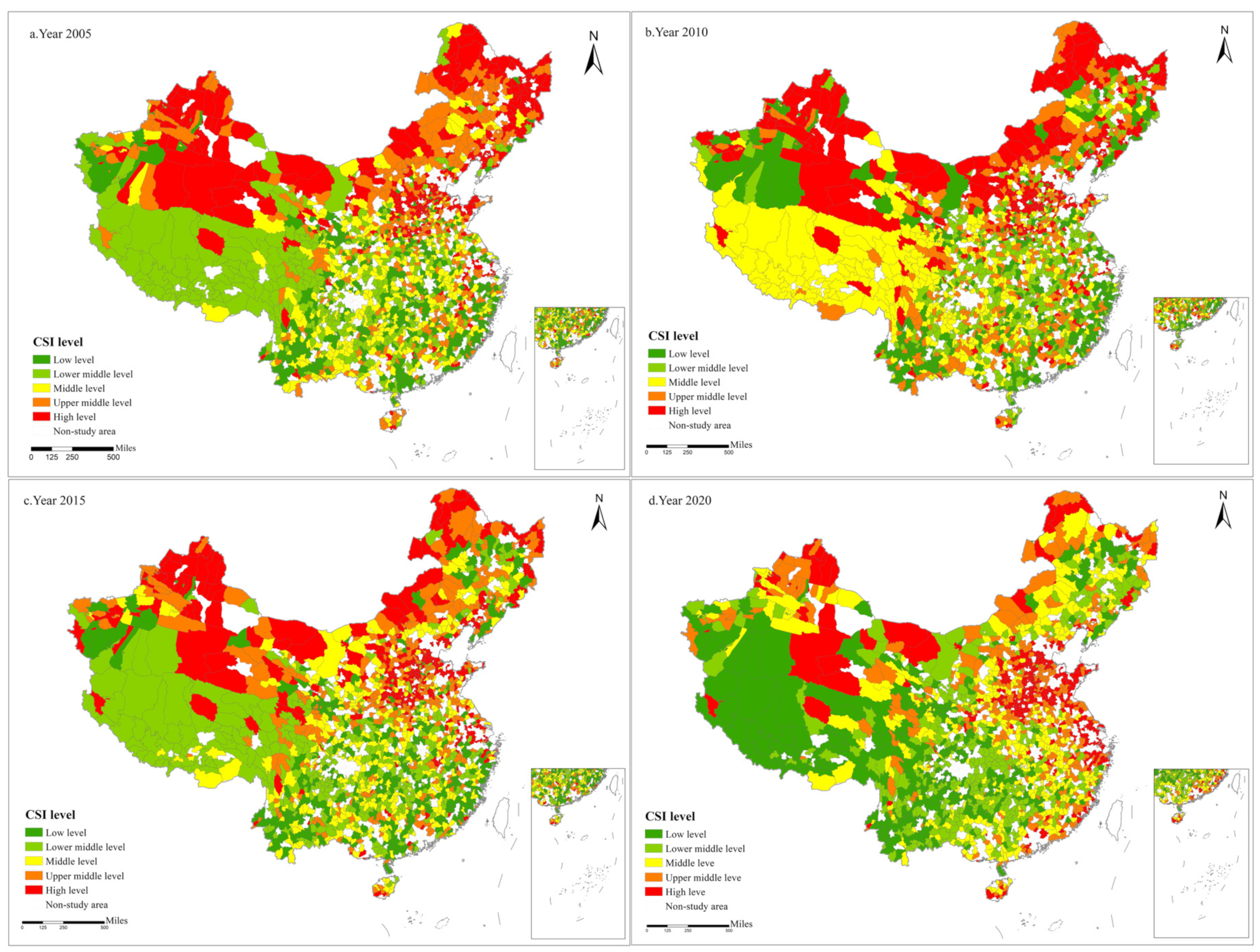
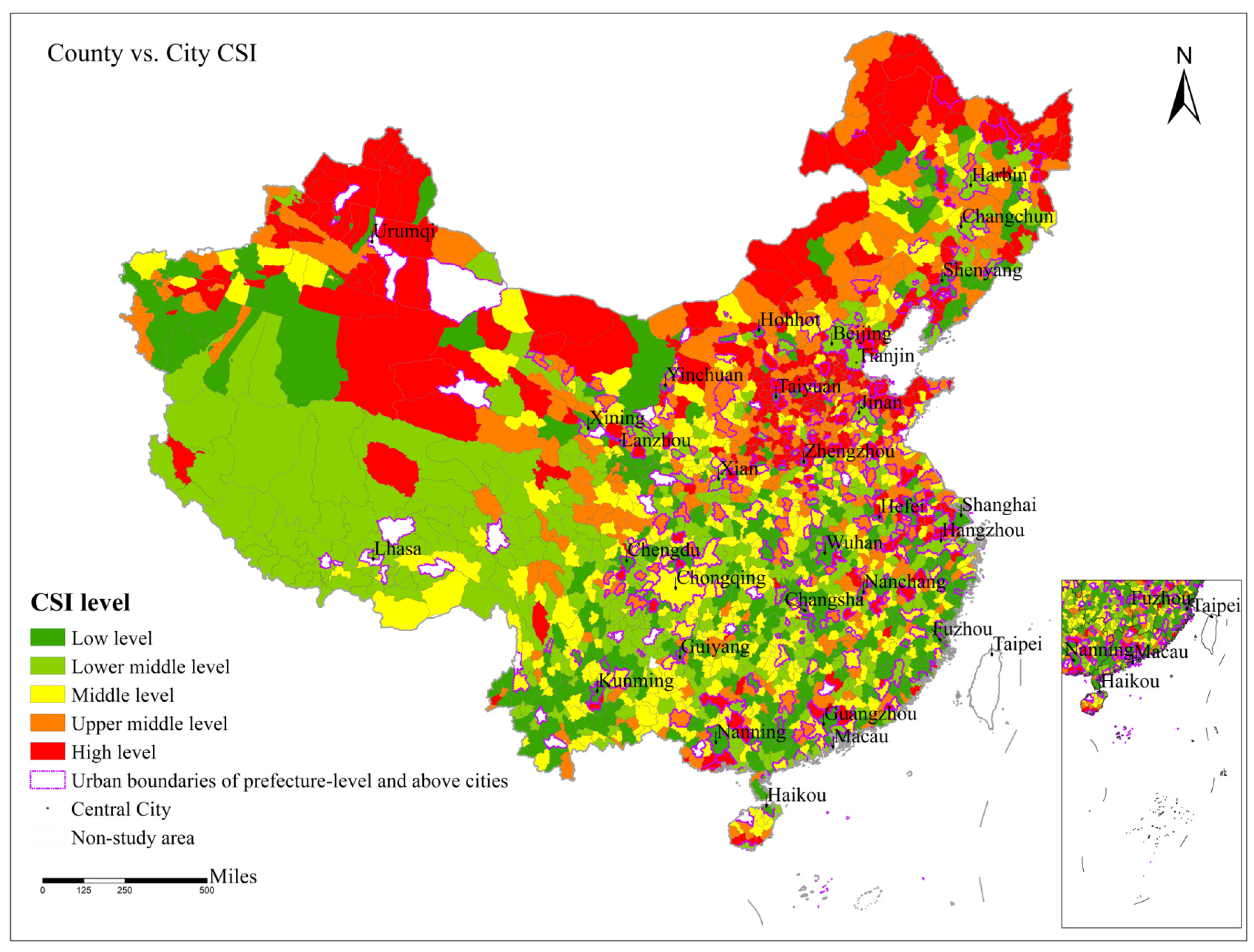
4.3.1. Spatial Distribution Patterns of County Sprawl

Firstly, the CSIs of 2005, 2010, 2015, and 2020 were spatially expressed using ArcGIS 10.8 software. On the basis of the calculated results, it was divided into five levels, namely low, lower medium, middle, upper medium, and high, indicating a CSI ranked at 0–20%, 20–40%, 40–60%, 60–80%, and 80–100% of the observed values, respectively (Figure 2). In 2005, the CSI showed a pattern of high in the north and low in the south. Most counties with high-level sprawl are located in North, Northeast, and Northwest China, including Liaoning, Jilin, Heilongjiang, Inner Mongolia, Xinjiang, Shanxi, Hebei, and the Shandong province. In 2010, the pattern of high in the north and low in the south remained unchanged, but the CSI in some counties in the northeast region decreased significantly. In 2015, The pattern of high CSI in the north and low in the south was modified, with the counties with high-level sprawl stretching to the south. In 2020, the number of counties with high-level sprawl in Zhejiang, Fujian, and Guangdong rose, and the spatial pattern of CSI changed from high in the north and low in the south to high in the east and low in the west. On this basis, the counties with high CSI were concentrated in the eastern coastal areas, including Hebei, Shandong, Jiangsu, Zhejiang, Fujian, and Guangdong, showing a gradually decreasing spatial pattern from east to west.

Second, the CSI of counties and municipal districts were compared spatially (Figure 3). From this, we can see that counties’ and municipal districts’ sprawl index had an interlocking distribution. In Figure 3, the sprawl index of first- and second-tier cities such as Beijing, Shanghai, Guangzhou, and Hangzhou was low. However, the sprawl index of many third- and fourth-tier cities in western China, such as Bazhong, Dingxi, Guigang, and Laibin, was high. Liu et al. [25] and Zhang et al. [28] reached similar conclusions to this study. However, this study found that highly sprawling counties surround central cities such as Beijing and Shanghai. In contrast, small and medium-sized cities with a high sprawl index are surrounded by counties with a low sprawl index, forming a contrast in the interlocking distribution.

To summarize, there are differences and connections between the sprawl of counties and municipal districts. Land resources are incredibly scarce in the municipal districts of central cities, resulting in high-density and high-intensity development patterns. At the same time, the surrounding counties have the advantage of the “borrowed scale,” which can attract more people, capital inflow, and enterprises to settle in the counties, but the laxer land use patterns bring about the counties’ sprawl. On the contrary, the spatial development of the municipal districts of small and medium-sized cities is still very rough, thus increasing their sprawl index. However, the surrounding counties have been influenced by the “shadow of agglomeration” and have lost their population and industry outward, and thus do not have the foundation to sprawl. It can be seen that even within the same urban administrative region, the levels of sprawl have apparent structural differences. The findings of this study are a valuable supplement to the existing research results and reflect the new characteristics of the spatial distribution patterns of urban sprawl after refinement to the county scale.

4.3.2. Territorial Spatial Dependency Patterns of County Sprawl

From the results of the global spatial dependence measure (

Table 1. Moran’s I calculation results for county sprawl.

Year	I-Value	z-Value	Year	I-Value	z-Value
2005	0.306 ***	7.158	2013	0.359 ***	8.776
2006	0.333 ***	3.108	2014	0.386 ***	8.602
2007	0.256 ***	6.126	2015	0.389 ***	5.327
2008	0.247 ***	4.171	2016	0.362 ***	7.361
2009	0.271 ***	5.560	2017	0.373 ***	8.547
2010	0.172 ***	7.791	2018	0.279 ***	6.274
2011	0.396 ***	8.795	2019	0.407 ***	9.260
2012	0.393 ***	6.103	2020	0.632 ***	8.340

Note: *** indicates significance at the 1% level.

), Moran’s index I ranged from 0.172 to 0.632 from 2005 to 2020, with the minimum value occurring in 2010 and the maximum value in 2020, and all years passed the significance test at the 1% level. This indicates that CSI has a significant positive spatial correlation, i.e., counties with high-level sprawl are adjacent to other counties with high-level sprawl. In contrast, counties with low-level sprawl surround counties with low-level sprawl, eventually forming a significant spatial dependence pattern. For 2005–2020, Moran’s index I showed a trend of increasing in fluctuation, indicating that the spatial dependence of CSI has been increasing.

Two significantly low Moran’s index I values were seen in 2010 and 2018. The lingering effects of the 2010 financial crisis may have caused this, while regulatory measures such as reducing the real estate inventory were implemented in counties in 2018. In the face of exogenous shocks such as the financial crisis and policy adjustments, the coping ability, means of coping, and policy implementation of different counties differed significantly, leading to a significant decrease in the spatial correlation of CSI. After this, Moran’s index I rebounded rapidly in 2011 and 2019, and its value exceeded that of previous years. This shows that exogenous shocks will only have a temporary impact, and fundamentally changing the evolutionary path of the CSI’s spatial dependence pattern is difficult.

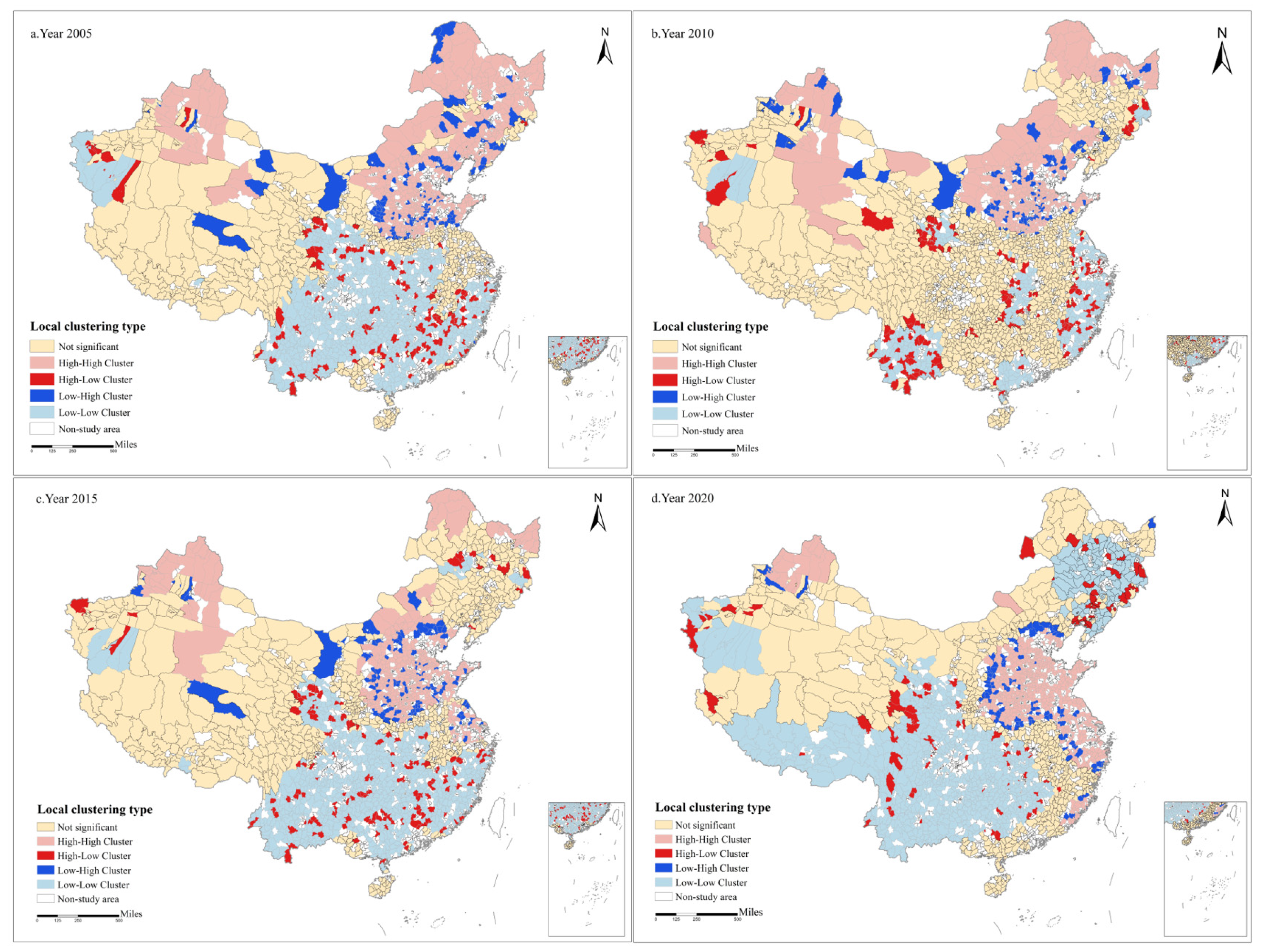
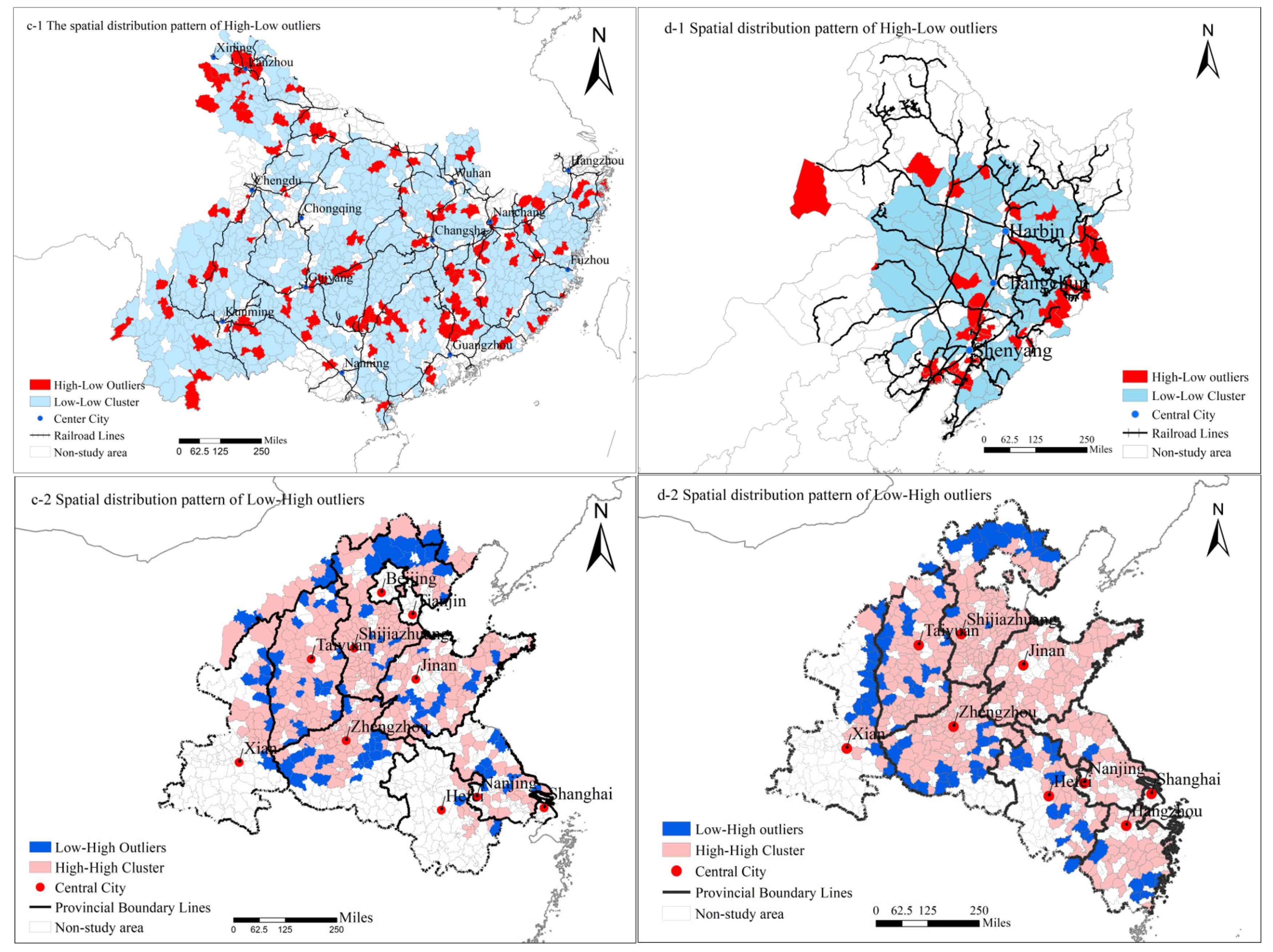
4.3.3. Local Spatial Clustering Pattern of County Sprawl

The global autocorrelation Moran’s index I can only identify whether CSI has a significant spatial clustering distribution from an overall perspective. However, we must reveal how, where, and why counties cluster. Therefore, to analyze the spatial clustering types and clustering areas of CSI more accurately and comprehensively, the local autocorrelation Moran’s index I was used to examine the spatial clustering patterns of CSI further (Figure 4).

High–high clusters refer to counties with a high CSI in themselves and in their surroundings. In 2005, the high–high cluster areas were distributed in the Northeast Plain, the North China Plain, and the Junggar Basin. The flat topography and the low elevation of the abovementioned areas contributed to the spatial clustering phenomenon of counties with high-level sprawl. In 2010, the high–high cluster range contracted slightly in the north. In 2015, the Northeast Plain withdrew from the high–high cluster areas; at the same time, the high–high cluster areas extended to the northern Zhejiang province. In 2020, the high–high cluster areas were mainly distributed in the North China Plain and the middle to lower Yangtze Plain. In summary, the high–high cluster areas were mainly concentrated in the plains during the observation period, and its range stopped to the north of the “Qinling–Huaihe” line. However, there was a tendency to extend southward on the eastern coast.

Low–low clusters refer to counties with a low CSI in themselves and in their surroundings. In 2005, the low–low cluster areas were mainly distributed in the southern region. It is easy to see that these areas have a complex topography, such as the Southeast Hills, Sichuan Basin, the Yunnan–Guizhou Plateau, and the Loess Plateau. As the population of counties gradually increases, the spatial constraints promote compact clustering of counties. In 2010, the low–low cluster areas contracted significantly. Immediately afterward, by 2015, the low–low cluster areas expanded again, especially starting to expand to the northeast. By 2020, the low–low cluster areas were widely distributed in the south and northeast.

High–low clusters refer to counties with a high CSI of their own and a low CSI in their surroundings. Using the years 2015 and 2020 in Figure 4 as examples, we explored the spatial distribution patterns of high–low outliers (as shown in Figure 5(c-1,d-1)). As seen in Figure 5(c-1), firstly, the high–low outliers were distributed in a point–line pattern along the main railway lines; secondly, the outliers were distributed in a cluster pattern at the railway intersections or near the central cities. Similarly, the spatial distribution pattern of high–low outliers in Figure 5(d-1) was more distinct. Most were located at railroad intersections, and the distribution was denser near the central cities.

Low–high clusters refer to counties with a low CSI of their own and a high CSI in their surroundings. Using 2015 and 2020 in Figure 4 as examples, we explored the spatial distribution patterns of low–high outliers (as shown in Figure 5(c-2,d-2)). According to Figure 5(c-2), the low–high outliers are mainly distributed along provincial boundaries. Chinese provincial boundaries are based on the shapes of the mountains and rivers. Therefore, the distribution of low–high outliers on provincial boundaries reflects the influence of geographic factors. Similarly, in Figure 5(d-2), the low–high outliers in 2020 spread further to the edges of the high–high cluster areas. The distribution on the provincial boundaries became more apparent, encircling the high–high cluster areas. The reason is easy to understand. A county in the plains has the conditions and motivation to sprawl. Thus, the high–high cluster areas continue to expand. However, when the high–high cluster areas encounter a topographic barrier and cannot continue to expand, several significant low–high outliers will form around it.

5. Driving Mechanisms of the Spatiotemporal Evolution of County Sprawl

5.1. Selection of Driving Factors

A system of drivers, shown in

Table 2. County sprawl drivers and their indicator calculations.

Driving Factors	Symbols	Indicators Calculation	Units
Level of economic development	ED	GDP per capita	million yuan
Industry structure	IS	Secondary industry added value/primary industry added value	%
Financial pressure	FP	General public budget expenditure/general public budget revenue	%
Population size	PZ	Number of permanent residents in the administrative area	Per person
Level of resident income	RI	Savings deposit balance per capita	yuan
Market vitality	MV	Year-end financial institutions’ loan balances/GDP	%
Terrain undulation	TU	Average terrain undulation by county based on 1 km × 1 km DEM raster data	—
Altitude	AL	Average altitude of each county calculated based on 1 km × 1 km DEM raster data	Meters
Distance to the nearest central city 4	DCC	Linear distance from the study unit to the nearest central city calculated using ArcGis 10.8 software	Kilometers
Distance to coastline	DC	Linear distance from the study unit to coastline calculated using ArcGis 10.8 software	Kilometers

, influencing the spatiotemporal evolution of county sprawl in China was developed on the basis of pertinent theories of regional economics and the new economic geography, as well as the advancement of extensive research on urban sprawl and urbanization [25,28,29,30].

The following drivers were selected.

(1)

Level of economic development. This reflects the strength or weakness of the county’s macro-economy.

(2)

Industrial structure. Industrialization drives the concentration of the population within counties and, at the same time, can enhance the efficiency of land use.

(3)

Financial pressure. The greater the financial pressure, the more likely the government will use land finance to compensate for the financial gap, leading to inefficient land use.

(4)

Population size. The population size is the basis of urbanization. The larger the population, the more potential for urbanization.

(5)

Level of residents’ income. As the income level of residents increases, people’s need for a better life becomes more urgent. For example, private cars can significantly expand the radius of people’s activities, which may impact the county’s sprawl.

(6)

Market vitality. This reflects the degree of economic activity in each county, which impacts urban construction.

(7)

Terrain undulation. A higher degree of terrain undulation is more costly for the spatial expansion of the county; therefore, it may promote a compact and intensive spatial form within the county.

(8)

Altitude. Areas with a higher altitude have poorer external connectivity and slower economic development. In addition, the higher the altitude, the higher the cost of county sprawl.

(9)

Distance to the nearest central city. The central city promotes economic growth and concentration of the population in the surrounding counties through the “borrowing scale”. However, it may also produce an agglomeration shadow, leading to the transfer of the county’ capital and population loss.

(10)

Distance to the coastline. An export-oriented economy is more likely to develop in areas closer to the coast, which benefits economic growth and efficient land use. Moreover, the closer the coastline, the more suitable the climate is for human habitation and the more attractive it is to the population [30].

5.2. Driver Detection Results

In line with the factor detection tool in GeoDetector, 2005, 2010, 2015, and 2020 were selected as observations to analyze each driver’s degree of influence and CSI ranking (

Table 3. Factor detection results for county sprawl drivers.

Driving Factors	2005		2010		2015		2020
	q-Value	Ranking	q-Value	Ranking	q-Value	Ranking	q-Value	Ranking
ED	0.103 **	8	0.173 ***	5	0.187 ***	6	0.205 ***	5
IS	0.181 ***	5	0.185 **	4	0.198 ***	5	0.201 ***	6
FP	0.172 **	6	0.162 *	6	0.140 ***	8	0.182 ***	8
PZ	0.312 ***	2	0.347 ***	1	0.322 ***	1	0.356 ***	1
RI	0.020	10	0.023 ***	10	0.024	9	0.015	9
MV	0.090 *	9	0.028 ***	9	0.003	10	0.004	10
TU	0.340 ***	1	0.306 ***	2	0.289 ***	2	0.280 ***	2
AL	0.240 ***	3	0.221 **	3	0.226 ***	3	0.218 ***	4
DCC	0.155 ***	7	0.120 ***	8	0.180 ***	7	0.195 ***	7
DC	0.210 ***	4	0.160 ***	7	0.209 ***	4	0.248 ***	3

Note: ***, **, and * indicate significance at the 1%, 5%, and 10% levels, respectively.

). According to Table 3, GeoDetector has a good ability to detect (a high q-value) the drivers of county sprawl each year, and most of the drivers passed the significance test.

Population size, terrain undulation, and altitude ranked as the top three. These factors are directly related to the core of county sprawl, i.e., the relationship between the population and land, especially in counties with larger populations and a flatter topography, which are highly prone to sprawl. The three drivers of distance to the coastline, industrial structure, and the level of economic development closely followed in the ranking. These reflect the county’s ability to gather resources and the dynamics of their economic growth, directly affecting the concentration of the population and development of the county’s infrastructure, significantly impacting county sprawl. Immediately afterwards, two drivers, namely financial pressure and distance to the nearest central city, ranked seventh to eighth in their impact on county sprawl. Financial pressure reflects the motives behind the county’s sprawl; the distance to the nearest central city reflects the conditions of the county for embedding in the urban network. These internal motivations and external conditions play a significant role in counties’ land supply and the concentration of their population, and thus significantly impact county sprawl. The two factors ranking last are the level of residents’ income and market vitality, which passed the significance test only in 2010. In response to the financial crisis, they have better explanatory power for county sprawl, while their role was weaker in other years.

The q-value of population size showed a fluctuating upward trend, indicating that the intensity of its influence on CSI has increased. In contrast, the q-values of terrain undulation and altitude have exhibited a general declining trend, demonstrating a decrease in the strength of these factors’ influence. At the same time, the q-values of five factors, including industrial structure and financial pressure, also showed an increasing trend, indicating that the intensity of their influence on CSI has increased. In summary, population size ranked first regarding both ranking and the degree of influence, indicating that it was the primary factor influencing the spatial divergence in county sprawl. The natural drivers, represented by terrain undulation and altitude, had a non-negligible influence on the spatial divergence of county sprawl. However, the intensity of their influence tended to decrease over time. Economic and spatial drivers, represented by the industrial structure, financial pressure, level of economic development, distance to a central city, and distance to the coastline, significantly influenced spatial divergence of county sprawl, and the intensity of their influence tended to increase. Therefore, the driving forces of county sprawl can be summarized as having four dimensions (natural, economic, social, and spatial drivers), and the four forces are interlinked and synergistic.

6. Conclusions and Discussion

6.1. Main Conclusions

This study took 1880 counties in China from 2005 to 2020 as the research object, measured CSI for the first time based on multi-source geographic raster data, and explored the characteristics of its spatiotemporal evolution and its driving mechanisms. The following main conclusions were obtained.

From 2005 to 2020, China’s CSI showed an upward trend. Controlling sprawl is a significant issue for counties during construction, as there is currently an undeniable tendency towards sprawl in counties. From the perspective of the temporal changes, the relationship between the population size and the supply of land determined the trend of CSI. Regarding regional heterogeneity, there is an apparent “Matthew effect” in the CSI, with the gap among different regions increasing over time. Regarding heterogeneity by administrative type, county-level cities are the critical targets for controlling sprawl.

From 2005 to 2020, the geographical pattern of CSI shifted from being high in the north to low in the south to being high in the east to low in the west. The levels of sprawl in counties and municipal districts are also significantly different, which is essential to account for in formulating differentiated land use policies. According to the spatial clustering patterns, high–high cluster areas are mainly distributed in the plains, while hilly, basin, and plateau areas tend to be low–low cluster areas. The high–low outliers are distributed in a point–line pattern along the railroad line and a clustering pattern near the railroad intersections or a central city. The low–high outliers encircle the high–high cluster areas, reflecting the blocking effect of geographical factors on the high–high clusters.

Regarding the driving mechanisms, population size ranks first in terms of impact and the intensity of this impact. The ranking of natural factors, represented by terrain undulation and altitude, was in the top three, but the intensity of their impact tended to decrease with time. Economic factors, such as industrial structure, financial pressure, and the level of economic development, and location factors, such as the distance to the coastline and the distance to the nearest central city, followed in the ranking, and the intensity of their impact showed an increasing trend. Based on this, natural, economic, social, and spatial drivers constitute the driving mechanism of the spatiotemporal evolution of county sprawl, and the four forces are interlinked and synergistic.

6.2. Discussion

The findings above are relevant to the promotion of high-quality county urbanization in China. Moreover, they have implications for formulating spatial development strategies for small cities in developing countries. The following insights emerged from this study.

First, the mode of economic development in the counties has been extensive, and attention needs to be paid to sprawl in the future. Previous studies considered that the sprawling phenomenon is more evident in large and medium-sized cities but did not pay attention to counties. However, due to their insufficient agglomeration, low land prices, insufficient regulation, and extensive development, counties may be characterized by more severe phenomena such as lax land use, waste of arable land resources, and a sprawling periphery. If we look at the developmental trajectory of global cities, once the sprawling development of cities is allowed to reach inertia, it is difficult to reverse the trend. Therefore, the development of counties should move forward incorporating lessons from the valuable experience of the construction of large cities, abandon the idea of “development by land,” establish a new concept of urbanization with people as the core, and promote the spatial layout of counties along a more reasonable track by improving spatial governance.

Second, the essence of county sprawl is an imbalance between the population and land, which is the key to controlling the sprawl. Within the county, urban managers should strengthen territorial spatial planning through the delineation of ecological, agricultural, and urban space; determining the redlines of ecological protection and arable land, and the boundaries of urban development; and the realization of intensive and efficient production spaces, livable and moderate living spaces, and ample and clear ecological spaces. It is necessary to re-evaluate the utilization efficiency of construction land in different counties and to scientifically and accurately configure the planned indicators of new construction land. At the same time, we should establish a mechanism linking the increases and decreases in construction land to the resident population, and thus reverse the mismatch between land elements among counties.

Third, we should classify and guide the high-quality development of various counties. Counties have differences in their economic, social, natural, and spatial factors, and their response to sprawl needs to be tailored to the local conditions. Economically developed or large cities surrounding counties should focus on the relationship between population inflows and land expansion and pay attention to the intensive use of land while continuing to attract population inflows. Counties with less developed economies or agricultural production areas need to speed up the improvement of the mechanism for the citizenship of transferred agricultural populations in the future and fully exploit their urbanization potential to promote population clustering. For functional counties with locational advantages for transportation, especially those near railroad lines, it is necessary to prevent the disorderly expansion of county towns brought about by the construction of new high-speed railway areas. For ecologically available counties with good natural endowments or counties with population outflows, we should follow the laws of nature and population flow to promote the transfer of the population to the surrounding large cities while reducing the supply of construction land and promoting smart contraction.

References

1. Jaeger, J.A.; Schwick, C. Improving the measurement of urban sprawl: Weighted Urban Proliferation (WUP) and its application to Switzerland. Ecol. Indic. 2014, 38, 294–308. [Google Scholar] [CrossRef]
2. Long, Y. Redefining Chinese city system with emerging new data. Appl. Geogr. 2016, 75, 36–48. [Google Scholar] [CrossRef]
3. Zhang, B.; Zhang, J.; Miao, C. Urbanization Level in Chinese Counties: Imbalance Pattern and Driving Force. Remote Sens. 2022, 14, 2268. [Google Scholar] [CrossRef]
4. Zhang, H.; Chen, M.; Liang, C. Urbanization of county in China: Spatial patterns and influencing factors. J. Geogr. Sci. 2022, 32, 1241–1260. [Google Scholar] [CrossRef]
5. Feng, Y.; Wang, X.; Du, W.; Liu, J.; Li, Y. Spatiotemporal characteristics and driving forces of urban sprawl in China during 2003–2017. J. Clean. Prod. 2019, 241, 118061. [Google Scholar] [CrossRef]
6. Harari, M. Cities in bad shape: Urban geometry in India. Am. Econ. Rev. 2020, 110, 2377–2421. [Google Scholar] [CrossRef]
7. Bento, A.M.; Cropper, M.L.; Mobarak, A.M.; Vinha, K. The effects of urban spatial structure on travel demand in the United States. Rev. Econ. Stat. 2005, 87, 466–478. [Google Scholar] [CrossRef]
8. Glaeser, E.L.; Gottlieb, J.D. Urban resurgence and the consumer city. Urban Stud. 2006, 43, 1275–1299. [Google Scholar] [CrossRef]
9. Rodríguez, M.C.; Dupont-Courtade, L.; Oueslati, W. Air pollution and urban structure linkages: Evidence from European cities. Renew. Sustain. Energy Rev. 2016, 53, 1–9. [Google Scholar] [CrossRef]
10. Bertram, C.; Goebel, J.; Krekel, C.; Rehdanz, K. Urban Land Use Fragmentation and Human Well-Being. Land Econ. 2022, 98, 399–420. [Google Scholar] [CrossRef]
11. Fallah, B.N.; Partridge, M.D.; Olfert, M.R. Urban sprawl and productivity: Evidence from US metropolitan areas. Pap. Reg. Sci. 2011, 90, 451–472. [Google Scholar] [CrossRef]
12. Fulton, W.B.; Pendall, R.; Nguyen, M.; Harrison, A. Who Sprawls Most? How Growth Patterns Differ across the US; Brookings Institution, Center on Urban and Metropolitan Policy: Washington, DC, USA, 2001.
13. Hamidi, S.; Ewing, R. A longitudinal study of changes in urban sprawl between 2000 and 2010 in the United States. Landsc. Urban Plan. 2014, 128, 72–82. [Google Scholar] [CrossRef]
14. Nazarnia, N.; Harding, C.; Jaeger, J.A. How suitable is entropy as a measure of urban sprawl? Landsc. Urban Plan. 2019, 184, 32–43. [Google Scholar] [CrossRef]
15. Li, G.; Li, F. Urban sprawl in China: Differences and socioeconomic drivers. Sci. Total Environ. 2019, 673, 367–377. [Google Scholar] [CrossRef]
16. Seevarethnam, M.; Rusli, N.; Ling, G.H.T.; Said, I. A geo-spatial analysis for characterising urban sprawl patterns in the Batticaloa municipal council, Sri Lanka. Land 2021, 10, 636. [Google Scholar] [CrossRef]
17. Horn, A.; Van Eeden, A. Measuring sprawl in the Western Cape Province, South Africa: An urban sprawl index for comparative purposes. Reg. Sci. Policy Pract. 2018, 10, 15–23. [Google Scholar] [CrossRef]
18. Ehrlich, M.V.; Hilber, C.A.; Schöni, O. Institutional settings and urban sprawl: Evidence from Europe. J. Hous. Econ. 2018, 42, 4–18. [Google Scholar] [CrossRef]
19. Nengroo, Z.A.; Bhat, M.S.; Kuchay, N.A. Measuring urban sprawl of Srinagar city, Jammu and Kashmir, India. J. Urban Manag. 2017, 6, 45–55. [Google Scholar] [CrossRef]
20. Wang, X.; Shi, R.; Zhou, Y. Dynamics of urban sprawl and sustainable development in China. Socio-Econ. Plan. Sci. 2020, 70, 100736. [Google Scholar] [CrossRef]
21. Yue, W.; Liu, Y.; Fan, P. Measuring urban sprawl and its drivers in large Chinese cities: The case of Hangzhou. Land Use Policy 2013, 31, 358–370. [Google Scholar] [CrossRef]
22. Tian, L.; Li, Y.; Yan, Y.; Wang, B. Measuring urban sprawl and exploring the role planning plays: A shanghai case study. Land Use Policy 2017, 67, 426–435. [Google Scholar] [CrossRef]
23. Guan, D.; He, X.; He, C.; Cheng, L.; Qu, S. Does the urban sprawl matter in Yangtze River Economic Belt, China? An integrated analysis with urban sprawl index and one scenario analysis model. Cities 2020, 99, 102611. [Google Scholar] [CrossRef]
24. Zhou, W.; Jiao, M.; Yu, W.; Wang, J. Urban sprawl in a megaregion: A multiple spatial and temporal perspective. Ecol. Indic. 2019, 96, 54–66. [Google Scholar] [CrossRef]
25. Liu, Z.; Liu, S.; Qi, W.; Jin, H. Urban sprawl among Chinese cities of different population sizes. Habitat Int. 2018, 79, 89–98. [Google Scholar] [CrossRef]
26. Jia, M.; Zhang, H.; Yang, Z. Compactness or sprawl: Multi-dimensional approach to understanding the urban growth patterns in Beijing-Tianjin-Hebei region, China. Ecol. Indic. 2022, 138, 108816. [Google Scholar] [CrossRef]
27. Liu, Y.; Fan, P.; Yue, W.; Song, Y. Impacts of land finance on urban sprawl in China: The case of Chongqing. Land Use Policy 2018, 72, 420–432. [Google Scholar] [CrossRef]
28. Zhang, X.; Pan, J. Spatiotemporal Pattern and Driving Factors of Urban Sprawl in China. Land 2021, 10, 1275. [Google Scholar] [CrossRef]
29. Wang, J.; Qu, S.; Peng, K.; Feng, Y. Quantifying urban sprawl and its driving forces in China. Discret. Dyn. Nat. Soc. 2019, 2019, 2606950. [Google Scholar] [CrossRef]
30. Rifat, S.A.A.; Liu, W. Quantifying spatiotemporal patterns and major explanatory factors of urban expansion in Miami Metropolitan Area during 1992–2016. Remote Sens. 2019, 11, 2493. [Google Scholar] [CrossRef] [Green Version]
31. Eren, F. Does the Asian property market work for sustainable urban developments? In Sustainable Cities in Asia; Caprotti, F., Yu, L., Eds.; Routledge: London, UK, 2018; pp. 32–47. [Google Scholar] [CrossRef]
32. Gao, B.; Huang, Q.; He, C.; Sun, Z.; Zhang, D. How does sprawl differ across cities in China? A multi-scale investigation using nighttime light and census data. Landsc. Urban Plan. 2016, 148, 89–98. [Google Scholar] [CrossRef]
33. Lv, Z.-Q.; Wu, Z.-F.; Wei, J.-B.; Sun, C.; Zhou, Q.-G.; Zhang, J.-H. Monitoring of the urban sprawl using geoprocessing tools in the Shenzhen Municipality, China. Environ. Earth Sci. 2011, 62, 1131–1141. [Google Scholar] [CrossRef]
34. Li, W.; Li, H.; Wang, S.; Feng, Z. Spatiotemporal Evolution of County Level Land Use Structure in the Context of Urban Shrinkage: Evidence from Northeast China. Land 2022, 11, 1709. [Google Scholar] [CrossRef]
35. Li, G.; Sun, S.; Fang, C. The varying driving forces of urban expansion in China: Insights from a spatial-temporal analysis. Landsc. Urban Plan. 2018, 174, 63–77. [Google Scholar] [CrossRef]
36. Henderson, J.V.; Nigmatulina, D.; Kriticos, S. Measuring urban economic density. J. Urban Econ. 2021, 125, 103188. [Google Scholar] [CrossRef]
37. Zhang, L.; Ren, Z.; Chen, B.; Gong, P.; Fu, H.; Xu, B. A Prolonged Artificial Nighttime-Light Dataset of China (1984–2020); National Tibetan Plateau/Third Pole Environment Data Center: Beijing, China, 2021. [Google Scholar] [CrossRef]
38. Li, Q.; Xu, Y.; Yang, X.; Chen, K. Unveiling the Regional Differences and Convergence of Urban Sprawl in China, 2006–2019. Land 2023, 12, 152. [Google Scholar] [CrossRef]
39. Qin, M.; Liu, X.; Tong, Y. Does Urban Sprawl Aggravate Smog Pollution? An Empirical Study of PM2. 5 in Chinese Cities. In A New Era: China’s Economy Globalizes; Palgrave MacMillan: Singapore, 2019; pp. 175–201. [Google Scholar]
40. Moran, P.A. Notes on continuous stochastic phenomena. Biometrika 1950, 37, 17–23. [Google Scholar] [CrossRef]
41. Zhao, R.; Zhan, L.; Yao, M.; Yang, L. A geographically weighted regression model augmented by Geodetector analysis and principal component analysis for the spatial distribution of PM2.5. Sustain. Cities Soc. 2020, 56, 102106. [Google Scholar] [CrossRef]
42. Zhao, Y.; Liu, L.; Kang, S.; Ao, Y.; Han, L.; Ma, C. Quantitative analysis of factors influencing spatial distribution of soil erosion based on geo-detector model under diverse geomorphological types. Land 2021, 10, 604. [Google Scholar] [CrossRef]
Figure 1. Time series trend of county sprawl.
Land 12 00721 g001
Figure 2. Spatial distribution pattern of county sprawl.
Land 12 00721 g002
Figure 3. Spatial distribution pattern of county sprawl and municipal districts sprawl.
Land 12 00721 g003
Figure 4. Local spatial clustering pattern of county sprawl.
Land 12 00721 g004
Figure 5. Spatial distribution pattern of county sprawl outliers.
Land 12 00721 g005