

Groundwater Urban Heat Island in Wrocław, Poland


1
Faculty of Geoengineering, Mining and Geology, Wroclaw University of Science and Technology, ul. Na Grobli 15, 50-421 Wroclaw, Poland
2
Independent Researcher, 65-395 Zielona Góra, Poland
*
Author to whom correspondence should be addressed.
Land 2023, 12(3), 658; https://doi.org/10.3390/land12030658
Submission received: 21 February 2023
/
Revised: 8 March 2023
/
Accepted: 9 March 2023
/
Published: 11 March 2023
(This article belongs to the Special Issue Urban Form and the Urban Heat Island Effect)
Abstract
:In the face of climate change and constantly progressing urbanization processes, so-called heat islands are observed with growing frequency. These phenomena are mainly characteristic of large cities, where increased air and land surface temperatures form an atmospheric (AUHI) or surface (SUHI) urban heat island (UHI). Moreover, UHIs have also been recognized in the underground environments of many cities worldwide, including groundwater (GUHI). However, this phenomenon is not yet as thoroughly studied as AUHI and SUHI. To recognize and characterize the thermal conditions beneath the city of Wrocław (SW, Poland), we analyze the groundwater temperature (GWT) of the first aquifer, measured in 64 wells in 2004–2005. The study aimed to identify groundwater urban heat islands (GUHI) in Wrocław. Therefore, we used a novel approach to gather data and analyze them in predefined seasonal periods. Meteorological data and satellite imagery from the same period allowed us to link GWT anomalies to the typical conditions that favor UHI formation. GWT anomaly related to the GUHI was identified in the central, urbanized part of Wrocław. Moreover, we found that the GUHI phenomenon occurs only seasonally during the winter, which is related to the city’s climate zone and anthropogenic heat sources. Comparing our results with previous works from other cities showed untypical behavior of the observed anomalies. In contrast to AUHI and SUHI temperatures, the GWT anomalies detected in Wrocław are characterized by seasonal transitions from a heat island in winter to a cold lake in summer. Such a transitional character of GUHI is described for the first time.
Keywords:
urban hydrogeology; thermal impact; subsurface temperature; climate change; land use; UHI; GUHI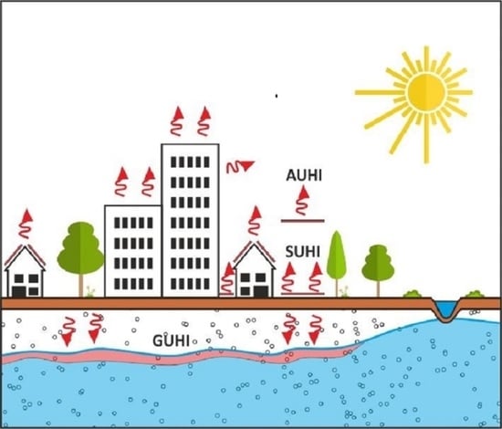
1. Introduction
Howard described the phenomenon of UHI for the first time in the XIX century [1] as an urban area significantly warmer than its surrounding rural areas due to human activities. Nowadays, we know that UHI can occur in the air (AUHI), on the surface (SUHI), and under the ground due to many artificial factors interfering.
The formation of an AUHI is facilitated by, among other things: large buildings [2,3,4], geographical location [5], topographical conditions [6,7,8], watercourses [9,10] and the lack of green areas [11,12]. These factors are responsible for the temperature difference between the AUHI and surrounding areas, reaching up to 12 °C [13]. The most commonly used AUHI survey method is a fixed and mobile weather station network [14,15]. Temperature measurements are obtained with a frequency ranging from several minutes to several hours and can reveal the spatial and temporal structure of an AUHI. A typical AUHI reaches its highest intensity 3–7 h after sunset [5,10,16,17], depending on the season.
The formation of SUHI results from changes in the urban energy balance. This phenomenon can be observed due to the dependence of remotely sensed land surface temperatures (LST) on air temperature [18,19,20]. The progress in this field of research allowed LST anomalies to be linked with changes in land cover/land use [21,22], changes in vegetation coverage [23,24,25] and many other factors, such as the presence of watercourses [10].
Since the thermal conditions below the surface are linked to surface conditions through conduction and advection [26], the UHI phenomenon can also be observed in GWT [27,28]. However, the coupling between air temperatures and GWT is not yet well explained [29,30]. In addition to air temperature, elevated GWT in a built-up area may be influenced by local hydrological conditions, such as downward groundwater flow [31], heat dissipation by the basements of buildings, district heating and sewerage infrastructure, or underground transportation infrastructure, such as metro and road tunnels [32,33].
Studies in Europe [28,34,35,36], Asia [37,38,39] and North America [40,41] have shown regional GWT increases of 2–5 °C. Studies using satellite data showed that satellite-derived LSTs could be used to approximate GWT in the shallow underground [42]. However, these observations are strongly dependent on weather conditions, especially snow cover and cloud cover [43], and the choice of convection [44,45] or convection-advection [46] as a model of heat conduction. This makes direct GWT measurements the most reliable source for information about the evolution of temperatures under the surface.
Based on other agglomerations’ examples, to complete the understanding of the heat transfer cycle related to urban development and climate change, it is crucial to analyze GUHI within the middle-east European city and deepen the knowledge of the GUHI in that part of Europe. In our work, we focused on GWT analysis beneath one of the largest Polish cities—the city of Wrocław (Figure 1), located in SW Poland (51° N, 17° E). There is no literature regarding the phenomenon of GUHI or SUHI in Wrocław. Thus, our research fills the knowledge gap. We recognized and characterized thermal conditions beneath Wrocław to identify and describe UHI in the city’s groundwater with specific underground conditions: distinctive geology and hydrogeology, no buildings with more than two underground levels, no deep road tunnels, no metro tunnels and relatively shallow other large underground infrastructure. We also received results not wholly similar to the previous works in other parts of Europe and the World. We believe sharing this knowledge is vital for further analyses of the GUHI phenomenon and planning future urban research.
During a series of studies conducted in Wroclaw in the early 2000s by Szymanowski et al. [7,16,43,47], the existence of an AUHI was confirmed. It occurred both in the early night hours and during the day in the summer and winter months. In 59% of the hours per year, the AUHI was observed with an intensity exceeding 0.5 °C. The most frequently observed temperature differences were between 0.5 °C and 3 °C. The highest observed temperature difference was 9.0 °C during the night on 12 December 1999. The same study highlighted the presence of an urban cold island (UCI). In this phenomenon, air temperatures observed in built-up areas are briefly lower than those in adjacent areas. UCI is typically explained by the thermal inertia of buildings [10,16] or the presence of large green areas in the city area [48]. In Wrocław, this phenomenon appeared sporadically in the early morning hours (12% of time annually) [16]. Another study conducted in 2011 [43] used satellite-derived LST and indicators such as the normalized difference vegetation index (NDVI) to analyze the most prominent cases of AUHI. It was found that the city’s green areas have a significant weakening effect on LST. This relationship can be observed in all world regions [24,48].
Despite the fact that AUHI has been fairly well documented in all major Polish metropolises: in Warsaw [49], Kraków [50], Poznań [19], Łódź [32,51] and Wrocław [7,16,43,47], the presence of the underground heat island has, in this part, of Europe has not been analyzed yet. Several works of researchers from the University of Wroclaw just touched on the topic of GWT beneath the city and municipal well-field [52,53] without deeper analysis of its character. We recognized and characterized thermal conditions beneath the city to identify and describe UHI in groundwater. Our study examines whether the UHI phenomenon occurs in the groundwater of Wrocław and answers the question of if the spatial distribution and temporal variability are visible. For this purpose, we analyzed GWT from the years 2004–2005. We used meteorological data and satellite images to compare GWT anomalies and UHI spatial structure. Examining previous research in Wrocław allowed us to analyze the course and time correlation of AUHI/SUHI and GWT anomalies, thus defining the GUHI phenomenon. This phenomenon is fundamental in the context of future research on the use of waste heat and the sustainable development of urban ecosystems. Therefore, this study may significantly contribute to establishing new ways to plan water management and low-heat geothermal energy systems in cities. The novelty of our research also lies in a spatial-seasonal GUHI analysis that has not been performed anywhere yet. This approach is slightly different from the spatial or statistical analysis used in all the existing studies from Europe and the World.
2. Characteristics of the Study Area
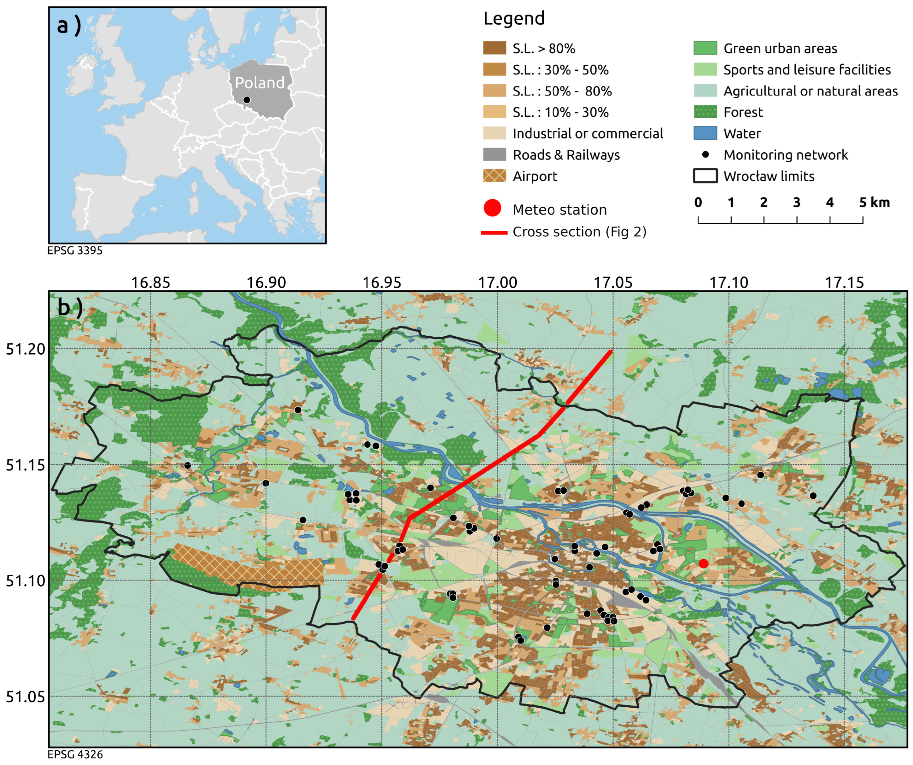
Wrocław is the fourth largest city in Poland and the capital of the Lower Silesian Voivodship. It covers an area of 293 km and is inhabited by ca. 640,000 people [54]. The city is located in the center of the Silesian Lowland, with the Odra River Valley crossing the city with a wide strip in the northwest/south-eastern direction. The city of Wroclaw is more than 1000 years old. It is closely connected with the Odra River and its numerous branches, tributaries and canals, including four other rivers (Widawa, Olawa, Sleza and Bystrzyca), that frame the city’s landscape and which, in combination with groundwater, create a unique hydraulic system. The length of the Odra River within the boundaries of Wroclaw is 26 km, and the width of its valley sometimes reaches several kilometers [55].
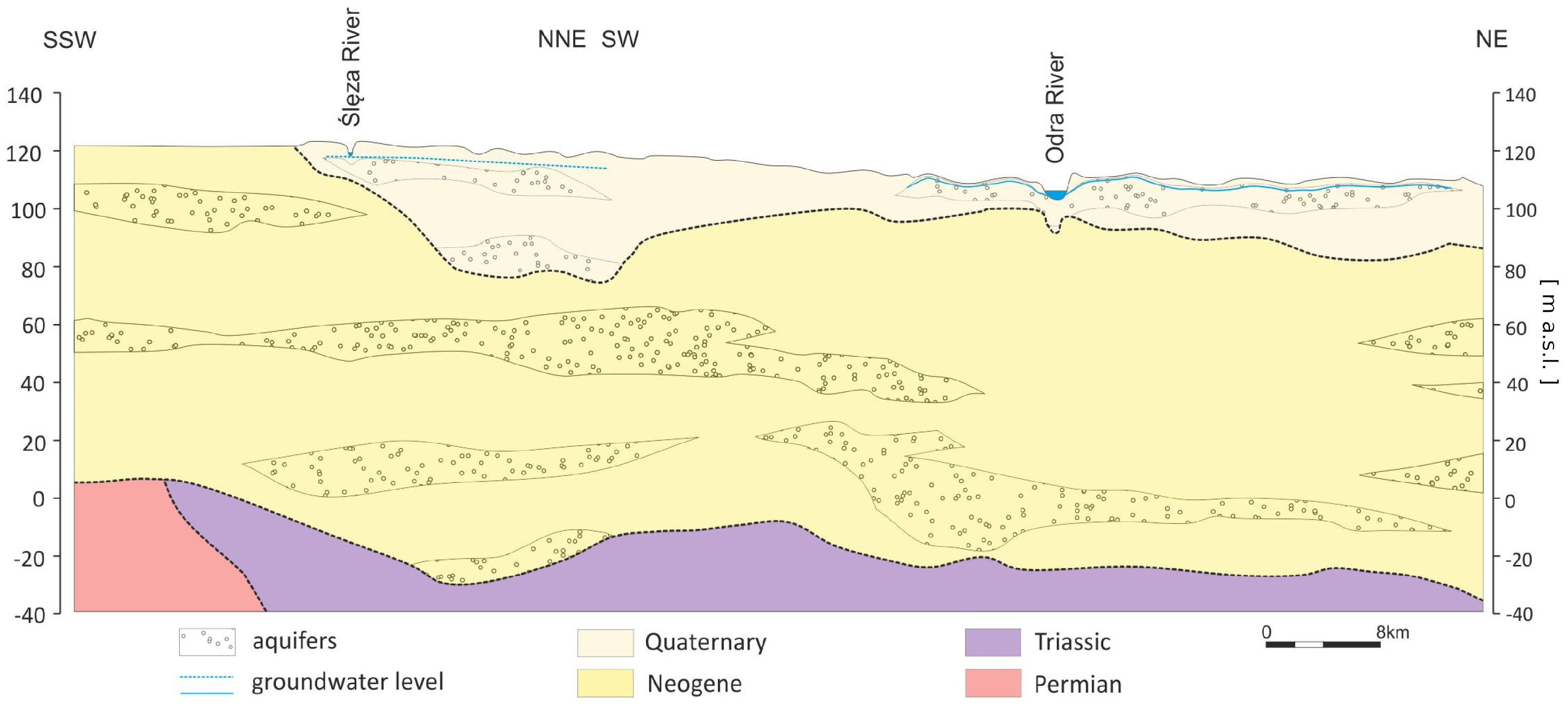
Geologically, Wrocław is situated on the southwestern margin of the Fore-Sudetic Monocline, adjacent to the Fore-Sudetic Block. The older, pre-Cenozoic tectonic basement (metamorphic shales and granite gneisses of the Middle Odra metamorphic, in places Lower Carboniferous rocks, Permian and Triassic formations) is covered with Cenozoic sediments represented by Neogene and Quaternary deposits. The basement is characterized by deep fractures and faults of several hundred meters, forming two dislocation systems—parallel and perpendicular to the direction of the Odra River [56]. Most of the city covers the Odra River valley filled with river sediments (Figure 2) except the southern districts on a moraine plateau composed of Quaternary fluvioglacial, glacial or Neogene sediments. Typically, the moraine upland clays have a thickness of 3–5 m and are discontinuous within the city’s borders. The first aquifer here is partially confined, and the groundwater table in this part of the city usually occurs below 2 m (Figure 2). The Odra Valley is filled mainly with permeable sediments, sands and gravels 20–50 m thick. The first aquifer is continuous and unconfined here, and the groundwater table is usually less than 5 m deep (Figure 2). The youngest deposits in the Wroclaw area are hardly permeable anthropogenic soils (historical and cultural layers) with thicknesses up to several meters, especially in the area of the city center [55,57].
The 2004 city of Wrocław could be described as a “green” city, where arable fields, wastelands, meadows and forests or parks were still present over a large area (Figure 1). The land use was divided between agricultural land (44.8%) and housing estates, communication and industrial areas (44.8%). The remaining few percent of the space was occupied mainly by forests and greenery (5.6%), water (3.4%), wastelands and mines (1.3% and 0.1%) [57]. Such repartition resulted from the gradual enlargement of the city in the 1950s and 1970s by the absorption of adjacent rural areas along with the entire rural structure of land development [55,58]. It should be noted, however, that densely urbanized areas and the entire infrastructure dominate the central and southern parts of the city: the oldest districts of Wrocław and new districts related to “large-panel” system buildings. Such an arrangement of urbanized areas causes the concentration and intensification of anthropogenic factors in these places, directly and indirectly impacting the city’s climate and groundwater. The massive use of impermeable construction materials in these areas significantly limits the possibility of free water circulation, including infiltration of rainfall and meltwater into the aquifer [57].
3. Materials and Methods
Observations of groundwater in aquifer layers beneath Wrocław were carried out from 13 April 2004, to 31 December 2005, in 99 wells. In the present article, we analyze data from 64 monitoring wells of the shallowest Quaternary aquifer, in which a total of 5184 temperature and groundwater depth measurements were taken. These measurements were collected once a week from 8 a.m. to 4 p.m. following a constant, planned itinerary. A gauge cable with a temperature probe of 0.01 °C resolution was used for temperature measurements. The measurements were made 1 m below the water table. A hydrogeological whistle was used to measure the position of the water table. The accuracy of the hydrogeological whistle was estimated to be 10 mm based on five consecutive measurements. The other 35 wells are not taken into consideration because of being set in a deep Tertiary aquifer or due to a lack of measurements that could not be running due to the destruction of the well.
Detailed information about the measurement points and selected parameters from the analysis are presented in Appendix B. Moreover, measurements from all 64 monitoring wells were made available along with the article under Open Data and presented in Supplementary Materials. These data have been compared with air temperature provided by an in situ meteorological station maintained by the Observatory of the Department of Climatology and Atmospheric Protection at the University of Wrocław (17°0520.0 E, 51°0619.0 N). It was the only meteo-station in the city that could provide us with meteorological observations parallel to the GWT measurements. The air temperature (Tair) was measured using a Vaisala HMP45AC probe equipped with a PT 100 temperature sensor having a measuring range of −40 °C to +60 °C.
Based on the seasonal variability of UHI presence in Wrocław [16], we also decided to analyze GUHI phenomena seasonally. The seasons are defined as follows: Summer 2004—from 4 July 2004 to 14 September 2004, Winter 2004/2005—from 1 February 2005 to 13 April 2005, and Summer 2005—from 8 July 2005 to 12 September 2005. These time intervals were determined based on the GWT time series analysis, which is shifted compared to air temperature. As with soil, the time lag will vary with the depth of the water table [59,60,61,62,63]. Based on previous studies, using lagged correlation [64,65], the phase shift between the GWT and Tair was calculated with an accuracy of 1 week, and it was estimated for 5–6 weeks of delay in GWT. To remove high-frequency noise from the GWT and air temperature time series, monthly means were presented in Figure 3.
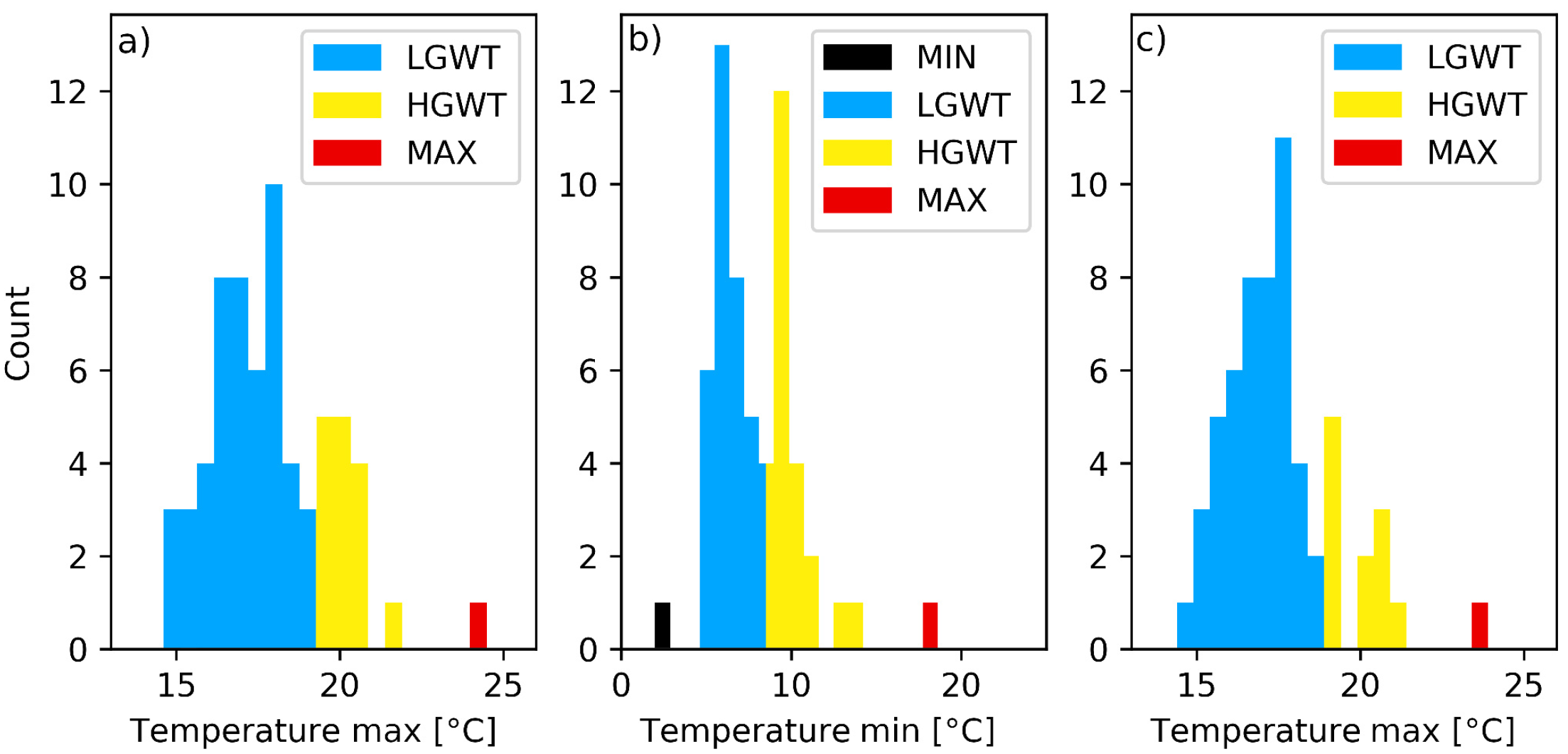
To confirm the presence of GUHI, the time evolution of mean monthly temperatures (Figure 3) and the seasonal distribution of maximal monthly GWT for the summer seasons and minimal GWT for the winter season (Figure 5) were examined. According to the literature [33,66], at least two data populations must be visible on the GWT histogram in the presence of UHI. The bi-modal distribution indicates that the data have come from two regions with different temperature ranges. Typically these regions are dense urban areas located inside the UHI zone, characterized by higher GWT mean, and areas located outside UHI, characterized by lower GWT mean [33,66,67]. It is necessary to separate these populations for spatial analysis using GIS software. This was performed with the help of a GWT histogram by determining the temperature threshold (Table 1) at the point where two populations overlap (Figure 5). The histogram also helps spot and isolate anomalies beyond the 3 distribution. In our case, four temperature groups were obtained. The following text describes these intervals as GWT minimum outliers (MIN), lower GWT (LGWT), higher GWT (HGWT) and GWT maximum outliers (MAX). The observation points were then assigned to one of the above-mentioned categories based on their average GWT in a given season.
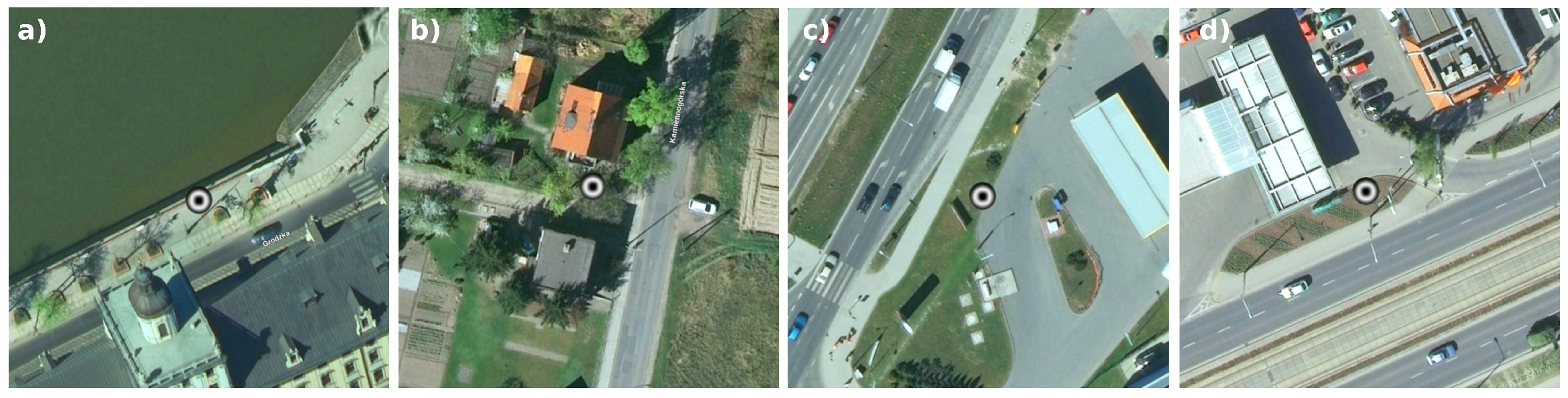
The observation points’ location data and their attributes were processed in QGIS. This allowed spatial analysis of selected attributes (Figure 4). Moreover, the geographical coordinates of each measurement point were used to identify the borehole position on high-resolution imagery and to describe the type of land cover/land use. This description was realized on 30 × 30 m image crops centered on the well. Screenshots presented in Figure 6 and Appendix A were made using Google Earth view, oriented to the north, at 249 m above sea level altitude. Finally, after receiving a spatial representation of GWT, the temporal evolution of the monthly GWT average was examined independently for LGWT (outside GUHI) and HGWT (inside GUHI) groups.
Visual identification and interpretation of land cover characteristics are sometimes used in UHI surveys [50,68,69]. This approach is because boreholes are almost always located within small green islets. At the same time, nearby buildings, passageways, concrete yards or parking lots are mostly responsible for heating up the terrain and air around these places. Information about vegetation cover or surface temperature in the vicinity of measuring points can be obtained by means of normalized difference vegetation index (NDVI) indices [70] or LST [71]. Depending on the type of urban areas and imagery resolution, the LST and NDVI data may correlate well, poorly or not at all with the UHI area [24,43,72]. Based on the preliminary GWT/LST analysis results, we found no reliable LST data to conduct a detailed analysis of both parameters. Thus it is not the scope of the article.
To characterize land cover/land use in the vicinity of wells, we focused on NDVI analysis. No high-resolution multispectral images are available for the period studied in the present article. For this reason, our research used data with 25 × 25 m and 30 × 30 m ground resolution from SPOT and IRSP6 instruments. The available data closest to the examined period is the IRSP6 image from 6 May 2006 and the SPOT image taken on 23 September 2006. Both photos were downloaded from the ESA Image2006 collection. The NDVI was estimated using QGIS software and Raster Calculator Tool in these squares with the observation well in the central point. For given GWT groups and seasons, the mean NDVI was calculated and is presented in Table 1.
The visual analysis of the land use was also performed to support NDVI analysis in the same squares. It was used for picturing the GWT classes of boreholes based on thresholds from Table 1 and in the background of land cover. A high-resolution satellite photo taken by MGPP Aero on 30 April 2009, available on Google Earth, was used for land use around the borehole description and is presented in Appendix A.
In both cases, there is a two or more years difference between the GWT measurements and the satellite images. In our work, we compared photo documentation from the time of measurements with the land use in the satellite images. We assumed no significant changes in the land cover in already urbanized areas during the 2004–2009 period. The photo documentation of the project, realized in 2004, was used to verify the location of the boreholes on satellite images and to clarify any doubts related to land development changes in 2004–2009.
4. Results
The average depth of the boreholes included in our work is 5.13 m (maximum 8.40 m, minimum 2.02 m). For technical reasons, the depth of some of the boreholes was not measured, but it is known from archival data that their depth did not exceed 20 m. The average water table depth below the ground level was 3.21 m during observation. Based on these numbers, we can conclude that all observation points are shallow wells, where GWT will be mainly regulated by anthropogenic heat and surface conditions [33,73].
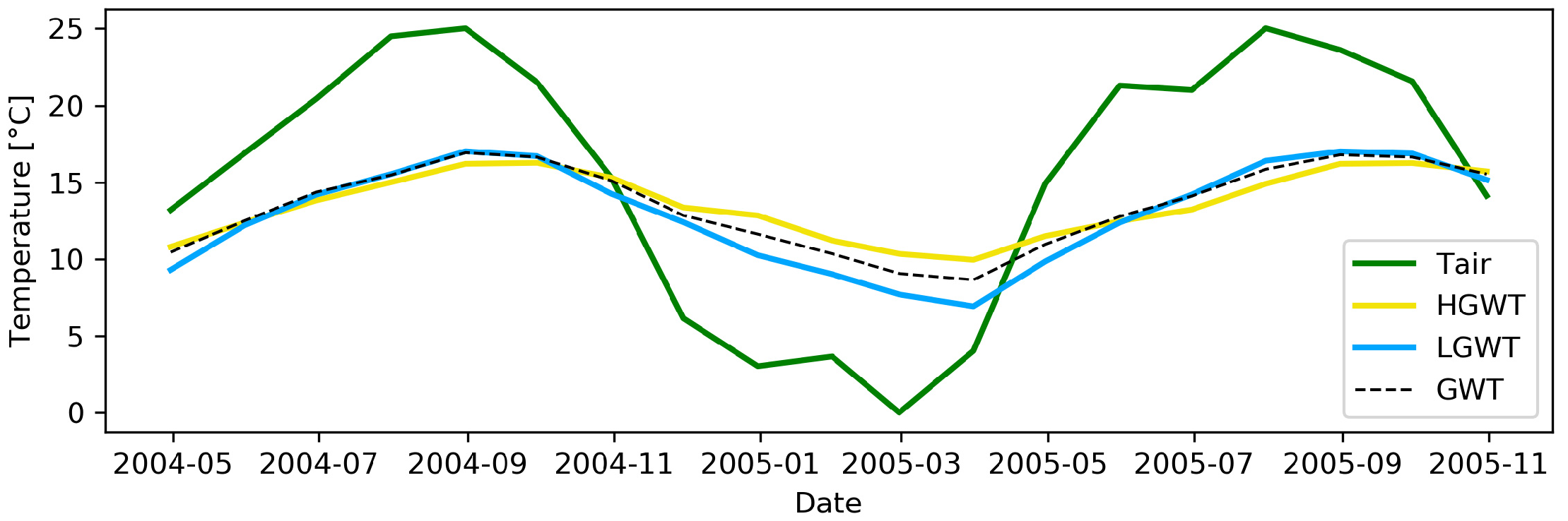
Figure 3 shows the monthly mean air temperature and the monthly GWT average from all measurement wells. The lowest mean monthly air temperature of −0.00 °C was recorded in February 2005, and the highest was 25.02 °C in July 2005. The lowest monthly GWT average of 8.64 °C was recorded in March 2005, and the highest was 16.92 °C in August 2004. Lagged correlation showed that air temperatures are 5 to 6 weeks ahead of GWT. This advance is constant over the entire measuring period.
Well depth and water table depth below the surface are also non-negligible factors. In wells where the water table is less than 10 m below the topographic surface (shallow wells according to the classification by Lee and Hahn [61]), the groundwater temperature is usually behind air temperature by 1–4 months. For example, Figura et al. [74] reported a time lag of 2–4 months for pumping wells with a median depth of groundwater table equal to 2.6, Clavache and Schneider [62,63] reported a time lag of 2–5 months for wells with a water table less than 10 m below the topographic surface. Finally, Masbruch et al. [59] obtained a time lag slightly longer than one month for a sensor suspended from the well cap to a depth of approximately 1.2 m. The time lag we received is, therefore, typical for shallow wells.
Figure 3 shows the histograms of the temperatures measured in the observation wells: minimum during winter and maximum during summer seasons. In all cases, we can observe a bimodal distribution. Such a distribution in urban conditions may be associated with the occurrence of UHI [33]. For each season, the measurement points were assigned to one of the four temperature groups: MIN, LGWT, HGWT and MAX (see Section 3). The exact thresholds for these temperature groups are shown in Table 1. A similar difference between the LGWT and HGWT temperature groups characterizes the winter and summer seasons. In 2005, the difference between the maximum LGWT population and the maximum HGWT population was 3.3 °C in winter and 3.5 °C in summer.
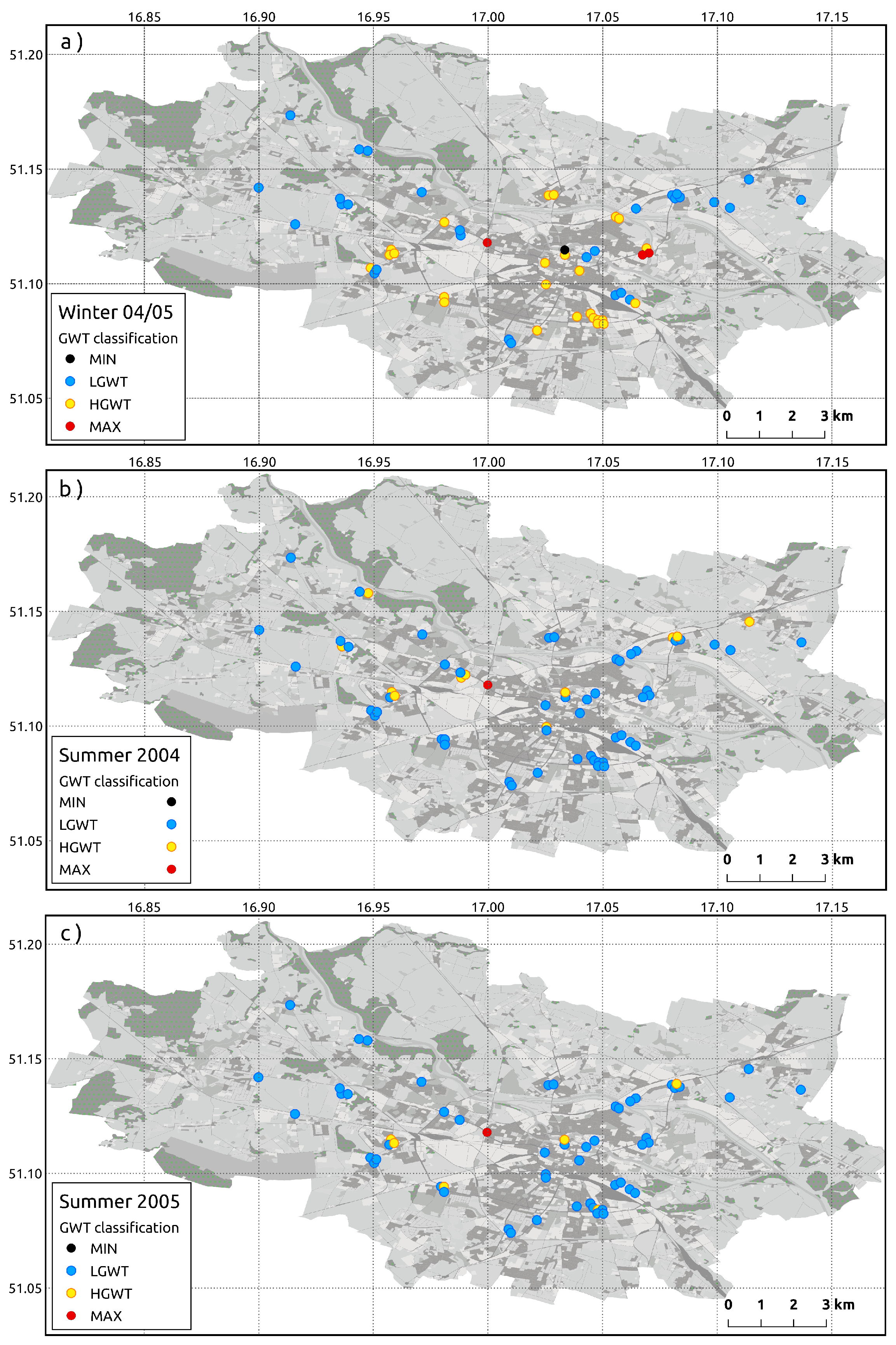
GUHI intensity is comparable in value to the GUHI observed in other agglomerations, such as Paris, Berlin or Karlsruhe [33,36,42], in which urban and hydrogeological and climate conditions are similar to Wrocław’s. The temperature difference between the LGWT and HGWT groups is practically the same in summer and winter. This peculiarity can be explained by the uneven spatial distribution of the monitoring network and the lack of measurement in many, especially densely built-up, districts (Figure 1). The next figure (Figure 4) shows the spatial distribution of the GWT anomalies. In winter 2004/2005 (Figure 4a), we can observe a concentration of the HGWT in the central part of the urbanized area. In this period, LGWT stations were located mainly on the city’s outskirts and in the low-rise districts. This kind of distribution is typical of GUHI occurring within large agglomerations [28,33,75,76]. In contrast to the winter period, in the summer of 2004 and 2005 (Figure 4b,c), we can observe a small number of HGWT observation points within the urbanized part of the city and a large number of observation points belonging to LGWT. This result suggests that the GUHI occurs only seasonally in winter and disappears in summer.
The NDVI analysis (Table 1) revealed that HGWT and MAX groups have a lower concentration of vegetation. The average NDVI value of the MAX group is typical for highly urbanized areas without tree cover. The average value of the LGWT group is typical for areas with large numbers of green features [24,72]. The date of the IRSP6 image coincides with the period of growth and flowering of plants and deciduous trees, which explains the higher NDVI means on this image. Similar NDVI values were also obtained for AUHI, including AUHI in Wrocław [43]. Low separation and high variance in the LGWT and HGWT groups excluded precise clustering of observation wells on the NDVI basis alone.
The analysis of the context of the surroundings partially confirms this discrepancy (Figure 6). The common feature for the HGWT group is the location of the well within human-transformed areas (Figure 6c). Typical locations are gas stations located along the main routes and parking lots. A complete lack of tree cover characterizes these measurement points. These conditions could theoretically translate to a higher GWT. The most common feature of the LGWT stations is their presence in low-rise areas with high participation of greenery (Figure 6b), which explains the higher NDVI mean in this group. In the LGWT group, however, many (12/30) points are located near gas stations (see Appendix A, Figure A3). Like the measurement points belonging to HGWT, they are located in an open area, close to highways and completely deprived of tree cover. This means that the increased temperatures in the HGWT group, thus GUHI, result from factors other than the surface temperature itself, which is also confirmed by the results of studies in other cities [33,38].
This discrepancy is also observed in the correlation between the HGWT and air temperature (Appendix B). In the HGWT group, this correlation is high ( > 0.75) for some of the measuring holes (11/26) and low ( < 0.6) for the rest of them. The evolution of the monthly GWT and Tair averages shown in Figure 5 shows that the annual GUHI behavior deviates from the behavior of the typical AUHI or SUHI described in the literature (see Introduction). By observing the LGWT and HGWT over the period from December 2004 to May 2005, we can see that the average temperature of the water in the wells in the urbanized part of the city (HGWT) is about 3 °C higher than the average temperature of in wells outside the GUHI (LGWT) area. During the summer period from July to September, these series are inverted. The average water temperature in wells located in the urbanized zone is about 0.5 °C lower than in holes outside this zone. This explains the inverted classification of the wells compared to the winter period (Figure 4b,c). The temperature transition is smooth. The data have shown that a similar transition also occurred in June 2004 and October 2005 (Figure 3). This suggests that the temperatures oscillated similarly before and after the period covered by our study. In conclusion, the city’s urbanized area has a cyclic seasonal transition of groundwater temperatures from GUHI to UCI.
5. Discussion
Our GWT analysis confirmed the presence of a heat island in the shallow groundwater (GUHI) of Wrocław, the main objective of our work. Due to the similarity of climatic conditions, the urbanization planning as well as the geology and hydrogeology of Wrocław to the German cities, such as Berlin or Karlsruhe [28,33], we expected to obtain a similar spatial distribution of GWT as in the above-mentioned cities. In general, our expectations were confirmed because the Wrocław GUHI is characterized by the highest intensity in the city center and is disappearing towards the outskirts and areas with lower building density (Figure 4a).
However, our analysis was realized using a different methodological approach than previous studies in Germany. We did not analyze the average annual temperatures but the average in two opposing seasons. First, for the summer period, when the typical SUHI, for example, in Berlin, is very intense and driven by solar radiation, and second for the winter period, when the classic SUHI is weaker, and GWT is mainly driven by anthropogenic heat [33,77]. With this approach, we noticed that the GUHI in Wrocław is the most intense in winter when the typical SUHI or AUHI is the weakest. This phenomenon can be likely explained by the influence of municipal infrastructure on shallow GWT and the heating period that starts in October and ends in April. We can suppose that this seasonality might result from the poor deep underground infrastructure of Wrocław, compared to the cities mentioned above, which could generate underground heat during the summer season, when winter households’ heating is off. Almost no buildings have more than two underground levels, no deep road tunnels, no metro tunnels or other large underground infrastructure. This also explains why the land cover/vegetation fraction analysis using satellite images was inconclusive. Moreover, we observed an interesting seasonal transition of the winter GUHI into UCI in the summer. A similar phenomenon was recorded in Wrocław and other cities concerning air or surface temperatures, but only on a daily cycle basis [16,77,78]. For example, during a study carried out in Wrocław in 1999–2000, Szymanowski observed the presence of both UHI and UCI. Both phenomena were very dynamic. A similar phenomenon was recorded in Wrocław and other cities noticed at different times of the day, all year long.
In the case of Wrocław’s groundwater, there is a cyclic formation of GUHI in the winter season and the progressive transition of the GUHI into a UCI of very low intensity in the summer (Figure 3). Therefore, the observed phenomenon differs from AUHI or UHI documented in Wrocław by Szymanowski using air temperatures and LST [16]. According to our research, the GUHI, unlike AUHI, is more intense during the winter and is much more stable. Changes in the GUHI are slow, possibly due to the thermal inertia of geological layers and heat accumulation in the shallow aquifer [79].
Of course, our research and analyses are biased by the short observation period (1 year), low frequency of tests (once a week), a relatively small number and uneven distribution of monitoring points (0.3 points/km). Nevertheless, many other analyses were based on short-term measurements, such as, for example, those in Germany [42]. This does not diminish the value of our observations, which are the first GWT analysis in Poland and contribute substantially to recognizing the GUHI phenomenon in the largest European cities. Our results also highlight the necessity of GUHI analysis with respect to seasonality adapted to the climate conditions in the region.
6. Conclusions and Perspectives
Our analysis identified a GWT anomaly related to the GUHI in the central, urbanized part of Wrocław. Moreover, we found that the GUHI phenomenon occurs only seasonally during winter, which relates to the city’s climate zone and anthropogenic heat sources. With the use of satellite imagery, we were able to confirm that a lower vegetation fraction characterizes areas with elevated GWT. However, neither the NDVI nor the air temperature was sufficient to delineate the GWT anomaly area. Nevertheless, the correlation of GWT with air temperature is very high for most stations ( 0.75 or better). In perspective, this correlation can be used to estimate GWT changes based on future climate projections. However, the analysis of land cover/land use near measuring points suggests that the elevated temperatures in the HGWT group do not depend exclusively on surface conditions.
Further research is, therefore, needed to better identify the GUHI phenomenon and the factors driving GWT. The analysis of the depth of the water table concerning the depth of the city’s underground infrastructure and the impact of the city’s extent on GWT seems to be the appropriate follow-up. The LST analysis and the inter-comparison of AUHI and GUHI spatiotemporal structure would also improve the understanding of the mechanisms and dependencies of these phenomena.
Supplementary Materials
The following are available online at https://www.mdpi.com/article/10.3390/land12030658/s1, data available in supplementary files—article_dataset.csv and google_earth.kml.
Author Contributions
Conceptualization, M.W.-K. and A.A.; methodology, A.A.; validation, M.W.-K.; formal analysis, M.W.-K.; investigation, M.W.-K.; resources, M.W.-K.; data curation, M.W.-K.; writing—original draft preparation, M.W.-K. and A.A.; writing—review and editing, M.W.-K. and A.A.; visualization, M.W.-K. and A.A.; supervision, M.W.-K.; project administration, M.W.-K.; funding acquisition, M.W.-K. All authors have read and agreed to the published version of the manuscript.
Funding
This research work was partially funded by an internal grant of the Institute of Geological Sciences, University of Wrocław no 20022/W/ING/04-59 and City of Wrocław MOZART program (InAquaCity project no BWU-29/2019/M8). It was also co-founded within the Polish Ministry of Education and Science funds granted to Wrocław University of Science and Technology for 2023.
Acknowledgments
This work could not have been performed without the data on air temperatures shared by the Observatory of the Department of Climatology and Atmospheric Protection at the University of Wrocław, satellite images from ESA Image 2006 collection and Google, MGPP Aero map data.
Conflicts of Interest
The author declares no conflict of interest. The funders had no role in the design of the study; in the collection, analyses, or interpretation of data; in the writing of the manuscript, or in the decision to publish the results.
Abbreviations
The following abbreviations are used in this manuscript:
| AUHI | atmospheric urban heat island; |
| GWT | groundwater temperatures; |
| GUHI | groundwater urban heat island; |
| LST | land surface temperatures; |
| NDVI | normalized difference vegetation index; |
| UHI | urban heat island; |
| UCI | urban cold island; |
| SUHI | surface urban heat island. |
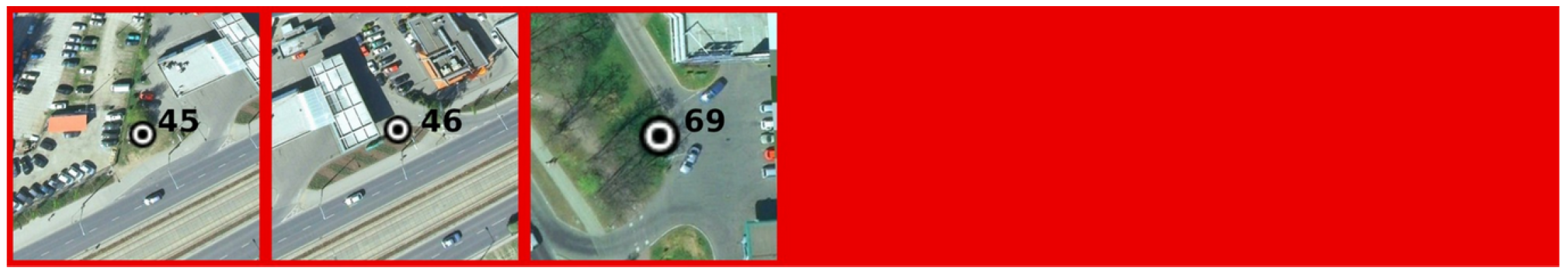
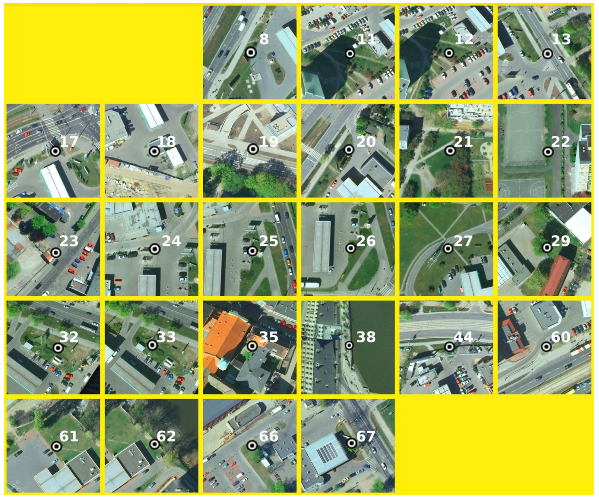
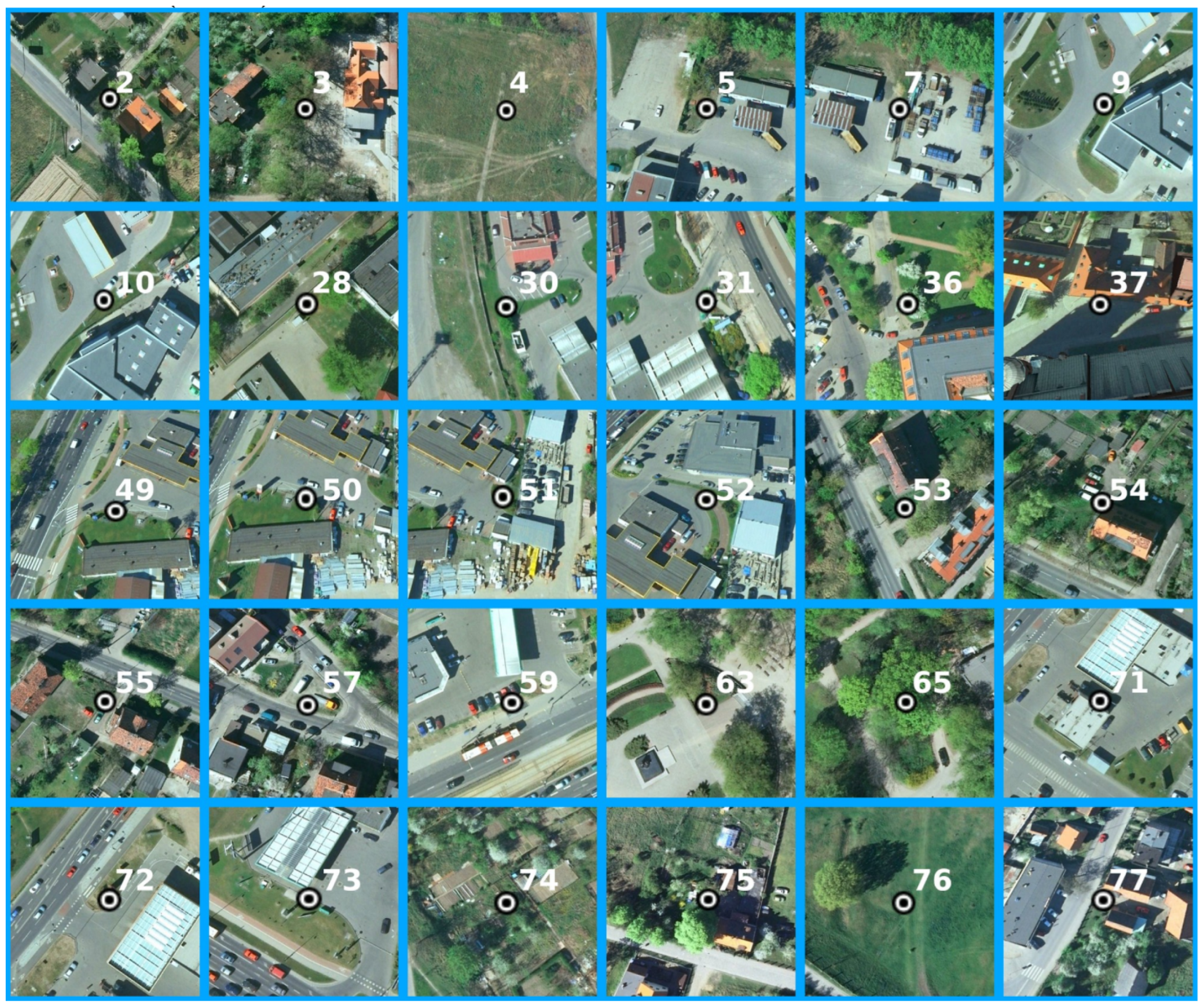
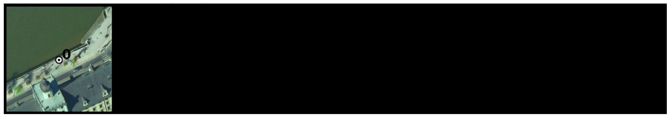
Appendix A
In order to describe the land use in the vicinity of the well, a high-resolution satellite photo taken by MGPP Aero on 30 April 2009, available on Google Earth, was used. Screenshots presented in this appendix were made using Google Earth view, oriented to the north, at 259 m above sea level altitude. The numbers next to wells are corresponding to UID in Table 1. The wells are classified seasonally using temperature intervals described in the Methodology (see Section 3). In total, four temperature intervals were obtained: GWT minimum outliers (MIN), lower GWT (LGWT), higher GWT (HGWT) and GWT maximum outliers (MAX). In the article, the HGWT group is assimilated to the GUHI. For the 2004/2005 winter season, we have obtained the following classification:
Figure A1.
GWT maximum outliers (MAX).

Figure A2.
Higher GWT (HGWT) assimilated to GUHI.

Figure A3.
Lower GWT (LGWT).

Figure A4.
GWT minimum outliers (MIN).

Appendix B

Table A1.
Detailed information on measuring points. Columns: 1—Unique ID, 2—Height above sea level (m), 3—Well depth (m), 4—Mean water table depth (m), 5—Longitude, 6—Latitude, 7—Linear regression R score (GWT vs. air temperature), 8—Slope, 9—Intercept, 10—Winter GWT classification, 11—Summer 2004 GWT classification, 12 Summer 2005 GWT classification. Results in columns 7–9 were obtained using Winter GWT classification (column 11). For wells with ID 17, 33 and 60, data from Summer 2005 (column 12) are missing (n.a.).
| 1 | 2 | 3 | 4 | 5 | 6 | 7 | 8 | 9 | 10 | 11 | 12 |
|---|---|---|---|---|---|---|---|---|---|---|---|
| 0 | 118.65 | 3.01 | 16.866563 | 51.149281 | 0.90 | 1.109 | −2.633 | MIN | HGWT | HGWT | |
| 71 | 116.57 | 4.49 | 2.14 | 16.987893 | 51.122601 | 0.84 | 2.112 | −15.377 | LGWT | LGWT | LGWT |
| 72 | 116.61 | 5.45 | 3.82 | 16.987780 | 51.122878 | 0.70 | 2.477 | −18.205 | LGWT | LGWT | LGWT |
| 74 | 111.23 | 2.02 | 1.18 | 16.970998 | 51.139932 | 0.88 | 1.947 | −10.950 | LGWT | LGWT | LGWT |
| 75 | 114.65 | 8.06 | 1.69 | 16.946866 | 51.158004 | 0.88 | 2.408 | −18.079 | LGWT | LGWT | LGWT |
| 76 | 110.99 | 2.94 | 1.73 | 16.943786 | 51.158694 | 0.87 | 2.763 | −18.383 | LGWT | LGWT | LGWT |
| 77 | 113.03 | 4.43 | 2.83 | 16.913755 | 51.173491 | 0.87 | 2.128 | −13.073 | LGWT | LGWT | LGWT |
| 2 | 118.84 | 6.20 | 1.27 | 16.899923 | 51.141886 | 0.83 | 2.518 | −18.389 | LGWT | LGWT | LGWT |
| 3 | 118.62 | 3.73 | 2.06 | 16.915804 | 51.125902 | 0.87 | 2.677 | −16.868 | LGWT | LGWT | LGWT |
| 5 | 117.26 | 4.23 | 2.25 | 16.937858 | 51.137295 | 0.82 | 2.098 | −16.181 | LGWT | LGWT | LGWT |
| 7 | 117.11 | 4.92 | 2.30 | 16.938388 | 51.137283 | 0.72 | 2.514 | −20.852 | LGWT | LGWT | LGWT |
| 4 | 116.19 | 4.25 | 2.81 | 16.936562 | 51.137225 | 0.87 | 2.300 | −13.439 | LGWT | LGWT | LGWT |
| 9 | 119.10 | 4.79 | 2.57 | 16.950364 | 51.105614 | 0.77 | 2.157 | −15.328 | LGWT | LGWT | LGWT |
| 10 | 119.03 | 4.67 | 2.54 | 16.950574 | 51.105752 | 0.76 | 2.821 | −21.413 | LGWT | LGWT | LGWT |
| 65 | 123.55 | 3.85 | 2.50 | 17.009241 | 51.075203 | 0.81 | 2.607 | −17.076 | LGWT | LGWT | LGWT |
| 63 | 124.13 | 4.32 | 2.88 | 17.009702 | 51.074778 | 0.70 | 3.241 | −23.233 | LGWT | LGWT | LGWT |
| 28 | 120.67 | 4.67 | 2.12 | 17.062957 | 51.092322 | 0.79 | 2.100 | −14.407 | LGWT | LGWT | LGWT |
| 30 | 119.76 | 1.65 | 17.056153 | 51.095442 | 0.80 | 1.770 | −10.522 | LGWT | LGWT | LGWT | |
| 31 | 119.51 | 1.40 | 17.056821 | 51.095514 | 0.78 | 2.336 | −17.413 | LGWT | LGWT | LGWT | |
| 36 | 118.90 | 4.71 | 3.53 | 17.043204 | 51.111568 | 0.88 | 3.312 | −27.471 | LGWT | LGWT | LGWT |
| 37 | 120.26 | 4.97 | 17.046442 | 51.114456 | 0.83 | 3.133 | −27.500 | LGWT | LGWT | LGWT | |
| 49 | 118.04 | 3.79 | 1.92 | 17.081856 | 51.138054 | 0.87 | 2.210 | −16.475 | LGWT | LGWT | LGWT |
| 50 | 118.17 | 3.63 | 2.02 | 17.082066 | 51.138025 | 0.80 | 2.117 | −13.031 | LGWT | LGWT | LGWT |
| 51 | 118.32 | 5.10 | 2.68 | 17.082444 | 51.138056 | 0.68 | 2.424 | −18.710 | LGWT | LGWT | LGWT |
| 52 | 118.43 | 3.20 | 2.15 | 17.082444 | 51.138453 | 0.78 | 1.972 | −13.463 | LGWT | HGWT | HGWT |
| 55 | 118.83 | 3.16 | 1.56 | 17.105609 | 51.133033 | 0.86 | 1.860 | −10.620 | LGWT | LGWT | LGWT |
| 54 | 117.66 | 6.45 | 1.69 | 17.098802 | 51.135477 | 0.20 | 3.534 | −27.919 | LGWT | LGWT | LGWT |
| 53 | 117.70 | 5.20 | 1.66 | 17.097671 | 51.136320 | 0.79 | 2.425 | −15.877 | LGWT | LGWT | LGWT |
| 57 | 122.60 | 3.09 | 1.61 | 17.113702 | 51.145718 | 0.87 | 1.745 | −10.260 | LGWT | LGWT | LGWT |
| 59 | 117.98 | 5.63 | 17.062763 | 51.131713 | 0.57 | 3.908 | −40.467 | LGWT | LGWT | LGWT | |
| 67 | 115.71 | 5.86 | 4.48 | 17.028512 | 51.138829 | 0.72 | 4.237 | −45.792 | HGWT | LGWT | LGWT |
| 66 | 115.76 | 5.68 | 4.27 | 17.027429 | 51.138567 | 0.45 | 3.453 | −29.766 | HGWT | LGWT | LGWT |
| 73 | 116.40 | 6.00 | 5.02 | 16.980919 | 51.126863 | 0.78 | 4.339 | −43.100 | HGWT | LGWT | LGWT |
| 11 | 120.53 | 7.12 | 2.81 | 16.957984 | 51.113298 | 0.84 | 3.367 | −39.965 | HGWT | HGWT | HGWT |
| 12 | 120.45 | 5.50 | 2.08 | 16.958122 | 51.113206 | 0.79 | 3.562 | −35.805 | HGWT | LGWT | LGWT |
| 13 | 120.77 | 5.00 | 1.58 | 16.958969 | 51.113386 | 0.79 | 2.363 | −20.639 | HGWT | HGWT | HGWT |
| 8 | 118.98 | 4.90 | 2.91 | 16.950131 | 51.105888 | 0.80 | 2.330 | −19.226 | HGWT | LGWT | LGWT |
| 17 | 124.07 | 4.08 | 16.979559 | 51.094236 | 0.84 | 4.551 | −48.499 | HGWT | LGWT | n.a. | |
| 18 | 123.94 | 2.08 | 16.979644 | 51.093770 | 0.86 | 2.792 | −26.864 | HGWT | HGWT | HGWT | |
| 19 | 125.33 | 4.49 | 16.980878 | 51.092403 | 0.76 | 4.764 | −47.638 | HGWT | LGWT | LGWT | |
| 20 | 124.70 | 7.40 | 5.00 | 17.021350 | 51.079639 | 0.68 | 4.444 | −42.821 | HGWT | LGWT | LGWT |
| 21 | 125.05 | 5.21 | 17.038807 | 51.085730 | 0.78 | 5.565 | −57.196 | HGWT | LGWT | LGWT | |
| 22 | 123.55 | 3.56 | 17.044782 | 51.086982 | 0.74 | 3.082 | −28.424 | HGWT | LGWT | LGWT | |
| 23 | 124.40 | 8.40 | 4.46 | 17.045010 | 51.085111 | 0.79 | 4.752 | −44.125 | HGWT | LGWT | LGWT |
| 24 | 124.53 | 4.27 | 17.048281 | 51.083742 | 0.60 | 2.218 | −12.890 | HGWT | HGWT | HGWT | |
| 25 | 124.67 | 4.71 | 17.048543 | 51.083611 | 0.39 | 0.195 | 3.264 | HGWT | LGWT | LGWT | |
| 26 | 124.76 | 4.98 | 17.048461 | 51.083473 | 0.31 | 4.501 | −38.734 | HGWT | LGWT | LGWT | |
| 27 | 124.76 | 4.82 | 17.050460 | 51.082405 | 0.53 | 3.846 | −32.446 | HGWT | LGWT | LGWT | |
| 29 | 120.86 | 7.28 | 2.32 | 17.063170 | 51.092141 | 0.63 | 4.704 | −41.051 | HGWT | LGWT | LGWT |
| 44 | 118.39 | 4.81 | 17.069237 | 51.114784 | 0.56 | 5.458 | −65.983 | HGWT | LGWT | LGWT | |
| 47 | 117.08 | 4.22 | 3.26 | 17.083378 | 51.115149 | 0.76 | 4.513 | −39.179 | HGWT | LGWT | LGWT |
| 60 | 117.65 | 5.32 | 17.062336 | 51.131606 | 0.50 | 17.120 | −198.137 | HGWT | LGWT | n.a. | |
| 61 | 116.97 | 7.35 | 3.63 | 17.056694 | 51.128397 | 0.53 | 3.417 | −27.884 | HGWT | LGWT | LGWT |
| 62 | 116.86 | 7.32 | 3.55 | 17.057143 | 51.128379 | 0.55 | 3.349 | −27.502 | HGWT | LGWT | LGWT |
| 38 | 118.65 | 5.48 | 3.26 | 17.033443 | 51.114156 | 0.68 | 4.090 | −38.072 | HGWT | LGWT | LGWT |
| 35 | 118.63 | 7.32 | 5.31 | 17.024546 | 51.109247 | 0.91 | 3.957 | −41.158 | HGWT | LGWT | LGWT |
| 32 | 119.37 | 2.02 | 17.025757 | 51.099291 | 0.87 | 2.649 | −23.069 | HGWT | LGWT | LGWT | |
| 33 | 119.44 | 1.92 | 17.025592 | 51.099321 | 0.82 | 3.081 | −24.697 | HGWT | LGWT | n.a. | |
| 69 | 116.57 | 7.46 | 4.23 | 16.999622 | 51.117932 | 0.82 | 5.512 | −104.462 | MAX | MAX | MAX |
| 46 | 118.58 | 5.24 | 17.069443 | 51.114341 | 0.57 | 11.484 | −152.314 | MAX | LGWT | LGWT | |
| 45 | 118.52 | 4.62 | 17.068759 | 51.114188 | 0.09 | 6.671 | −81.956 | MAX | LGWT | LGWT |
MIN, GWT minimum outliers; LGWT, lower GWT group; HGWT, higher GWT group; MAX, GWT maximum outliers.
References
- Howard, L. Climate of London Deduced from Meteorological Observations, 1833rd ed.; Harvey and Darton: London, UK, 1833; Volume 1–3. [Google Scholar]
- Bennet, M.G.; Ewenz, C. Increased urban heat island effect due to building height increase. In Proceedings of the MODSIM2013, 20th International Congress on Modelling and Simulation; Piantadosi, J., Anderssen, R.S., Boland, J., Eds.; Modelling and Simulation Society of Australia and New Zealand (MSSANZ), Inc.: Canberra, Australia, 2013. [Google Scholar] [CrossRef]
- Bakarman, M.A.; Chang, J.D. The Influence of Height/width Ratio on Urban Heat Island in Hot-arid Climates. Procedia Eng. 2015, 118, 101–108. [Google Scholar] [CrossRef]
- Li, Y.; Schubert, S.; Kropp, J.P.; Rybski, D. On the influence of density and morphology on the Urban Heat Island intensity. Nat. Commun. 2020, 11, 2647. [Google Scholar] [CrossRef]
- Oke, T.R. The energetic basis of the urban heat island. Q. J. R. Meteorol. Soc. 1982, 108, 1–24. [Google Scholar] [CrossRef]
- Oke, T.R. Canyon geometry and the nocturnal urban heat island: Comparison of scale model and field observations. J. Climatol. 1981, 1, 237–254. [Google Scholar] [CrossRef]
- Szymanowski, M. Interactions between thermal advection in frontal zones and the urban heat island of Wrocław, Poland. Theor. Appl. Climatol. 2005, 82, 207–224. [Google Scholar] [CrossRef]
- Suder, A.; Szymanowski, M. Determination of Ventilation Channels in Urban Area: A Case Study of Wrocław (Poland). Pure Appl. Geophys. 2014, 171, 965–975. [Google Scholar] [CrossRef] [Green Version]
- Hathway, E.A.; Sharples, S. The interaction of rivers and urban form in mitigating the Urban Heat Island effect: A UK case study. Build. Environ. 2012, 58, 14–22. [Google Scholar] [CrossRef] [Green Version]
- Moyer, A.N.; Hawkins, T.W. River effects on the heat island of a small urban area. Urban Clim. 2017, 21, 262–277. [Google Scholar] [CrossRef]
- Aram, F.; García, E.H.; Solgi, E.; Mansournia, S. Urban green space cooling effect in cities. Heliyon 2019, 5. [Google Scholar] [CrossRef] [Green Version]
- Huang, M.; Cui, P.; He, X. Study of the Cooling Effects of Urban Green Space in Harbin in Terms of Reducing the Heat Island Effect. Sustainability 2018, 10, 1101. [Google Scholar] [CrossRef] [Green Version]
- Hawkins, T.W.; Brazel, A.J.; Stefanov, W.L.; Bigler, W.; Saffell, E.M. The Role of Rural Variability in Urban Heat Island Determination for Phoenix, Arizona. J. Appl. Meteorol. 2004, 43, 476–486. [Google Scholar] [CrossRef]
- Voogt, J.A.; Oke, T.R. Thermal remote sensing of urban climates. Remote Sens. Environ. 2003, 86, 370–384. [Google Scholar] [CrossRef]
- Oke, T.R. Initial Guidance to Obtain Representative Meteorological Observations at Urban Sites; World Meteorological Organization: Geneva, Switzerland, 2004. [Google Scholar]
- Szymanowski, M. Miejska Wyspa Ciepła We Wrocławiu; Wydawnictwo Uniwersytetu Wrocławskiego: Wrocław, Poland, 2004. [Google Scholar]
- Tan, M.; Li, X. Quantifying the effects of settlement size on urban heat islands in fairly uniform geographic areas. Habitat Int. 2015, 49, 100–106. [Google Scholar] [CrossRef]
- Martin, P.; Baudouin, Y.; Gachon, P. An alternative method to characterize the surface urban heat island. Int. J. Biometeorol. 2015, 59, 849–861. [Google Scholar] [CrossRef]
- Majkowska, A.; Kolendowicz, L.; Półrolniczak, M.; Hauke, J.; Czernecki, B. The urban heat island in the city of Poznań as derived from Landsat 5 TM. Theor. Appl. Climatol. 2017, 128, 769–783. [Google Scholar] [CrossRef] [Green Version]
- Das, P.; Vamsi, K.S.; Zhenke, Z. Decadal Variation of the Land Surface Temperatures (LST) and Urban Heat Island (UHI) over Kolkata City Projected Using MODIS and ERA-Interim DataSets. Aerosol Sci. Eng. 2020, 4, 200–209. [Google Scholar] [CrossRef]
- Makinde, E.O.; Agbor, C.F. Geoinformatic assessment of urban heat island and land use/cover processes: A case study from Akure. Environ. Earth Sci. 2019, 78, 483. [Google Scholar] [CrossRef]
- Karakuş, C.B. The Impact of Land Use/Land Cover (LULC) Changes on Land Surface Temperature in Sivas City Center and Its Surroundings and Assessment of Urban Heat Island. Asia-Pac. J. Atmos. Sci. 2019, 55, 669–684. [Google Scholar] [CrossRef]
- Santamouris, M. Cooling the cities—A review of reflective and green roof mitigation technologies to fight heat island and improve comfort in urban environments. Sol. Energy 2014, 103, 682–703. [Google Scholar] [CrossRef]
- Grover, A.; Singh, R.B. Analysis of Urban Heat Island (UHI) in Relation to Normalized Difference Vegetation Index (NDVI): A Comparative Study of Delhi and Mumbai. Environments 2015, 2, 125–138. [Google Scholar] [CrossRef] [Green Version]
- Yang, Q.; Huang, X.; Li, J. Assessing the relationship between surface urban heat islands and landscape patterns across climatic zones in China. Sci. Rep. 2017, 7, 9337. [Google Scholar] [CrossRef] [PubMed] [Green Version]
- Cheon, J.Y.; Ham, B.S.; Lee, J.Y.; Park, Y.; Lee, K.K. Soil Temperatures in Four Metropolitan Cities of Korea from 1960 to 2010: Implications for Climate Change and Urban Heat; Springer: Berlin, Germany, 2014; Volume 71, pp. 5215–5230. [Google Scholar]
- Zhu, K.; Blum, P.; Ferguson, G.; Balke, K.D.; Bayer, P. The geothermal potential of urban heat islands. Environ. Res. Lett. 2010, 5, 044002. [Google Scholar] [CrossRef]
- Menberg, K.; Bayer, P.; Zosseder, K.; Rumohr, S.; Blum, P. Subsurface urban heat islands in German cities. Sci. Total. Environ. 2013, 442, 123–133. [Google Scholar] [CrossRef] [PubMed]
- Beltrami, H.; Kellman, L. An examination of short- and long-term air–ground temperature coupling. Glob. Planet. Chang. 2003, 38, 291–303. [Google Scholar] [CrossRef]
- Dědeček, P.; Šafanda, J.; Rajver, D. Detection and quantification of local anthropogenic and regional climatic transient signals in temperature logs from Czechia and Slovenia. Clim. Chang. 2012, 113, 787–801. [Google Scholar] [CrossRef]
- Kurylyk, B.L.; MacQuarrie, K.T.B. A new analytical solution for assessing climate change impacts on subsurface temperature. Hydrol. Process. 2014, 28, 3161–3172. [Google Scholar] [CrossRef]
- Fortuniak, K. Miejska Wyspa Ciepła: Podstawy Energetyczne, Studia Eksperymentalne, Modele Numeryczne i Statystyczne. Ph.D. Thesis, Wydaw. UŁ, Łódź, Poland, 2003. ISBN 9788371716584. [Google Scholar]
- Benz, S. Human Impact on Groundwater Temperatures; Karlsruher Institut für Technologie: Karlsruhe, Germany, 2016. [Google Scholar] [CrossRef]
- Balke, K.D. Die Grundwassertemperaturen in Ballungsgebieten; Institutional Reasearch Report T81-028; Geologisches Landratsamt Nordrhein: Westfahlen, Germany, 1981. [Google Scholar]
- Čermák, V.; Bodri, L.; Šafanda, J.; Krešl, M.; Dědeček, P. Ground-air temperature tracking and multi-year cycles in the subsurface temperature time series at geothermal climate-change observatory. Stud. Geophys. Geod. 2014, 58, 403–424. [Google Scholar] [CrossRef]
- Perrier, F.; Mouël, J.L.L.; Poirier, J.P.; Shnirman, M.G. Long-term climate change and surface versus underground temperature measurements in Paris. Int. J. Climatol. 2005, 25, 1619–1631. [Google Scholar] [CrossRef]
- Taniguchi, M.; Shimada, J.; Fukuda, Y.; Yamano, M.; Onodera, S.i.; Kaneko, S.; Yoshikoshi, A. Anthropogenic effects on the subsurface thermal and groundwater environments in Osaka, Japan and Bangkok, Thailand. Sci. Total Environ. 2009, 407, 3153–3164. [Google Scholar] [CrossRef]
- Huang, S.; Taniguchi, M.; Yamano, M.; Wang, C.h. Detecting urbanization effects on surface and subsurface thermal environment—A case study of Osaka. Sci. Total Environ. 2009, 407, 3142–3152. [Google Scholar] [CrossRef]
- Yamano, M.; Goto, S.; Miyakoshi, A.; Hamamoto, H.; Lubis, R.F.; Monyrath, V.; Taniguchi, M. Reconstruction of the thermal environment evolution in urban areas from underground temperature distribution. Sci. Total Environ. 2009, 407, 3120–3128. [Google Scholar] [CrossRef]
- Wang, K.; Lewis, T.J.; Belton, D.S.; Shen, P.Y. Differences in recent ground surface warming in eastern and western Canada: Evidence from borehole temperatures. Geophys. Res. Lett. 1994, 21, 2689–2692. [Google Scholar] [CrossRef]
- Ferguson, G.; Woodbury, A.D. Urban heat island in the subsurface. Geophys. Res. Lett. 2007, 34. [Google Scholar] [CrossRef]
- Benz, S.A.; Bayer, P.; Goettsche, F.M.; Olesen, F.S.; Blum, P. Linking Surface Urban Heat Islands with Groundwater Temperatures. Environ. Sci. Technol. 2016, 50, 70–78. [Google Scholar] [CrossRef] [PubMed]
- Szymanowski, M.; Kryza, M. Application of remotely sensed data for spatial approximation of urban heat island in the city of Wrocław, Poland. In Proceedings of the 2011 Joint Urban Remote Sensing Event, Munich, Germany, 11–13 April 2011; pp. 353–356. [Google Scholar] [CrossRef]
- Pollack, H.N.; Huang, S.; Shen, P.Y. Climate Change Record in Subsurface Temperatures: A Global Perspective. Science 1998, 282, 279–281. [Google Scholar] [CrossRef] [Green Version]
- Beltrami, H.; Bourlon, E.; Kellman, L.; González-Rouco, J.F. Spatial patterns of ground heat gain in the Northern Hemisphere. Geophys. Res. Lett. 2006, 33. [Google Scholar] [CrossRef] [Green Version]
- Bense, V.; Beltrami, H. Impact of horizontal groundwater flow and localized deforestation on the development of shallow temperature anomalies. J. Geophys. Res. Earth Surf. 2007, 112. [Google Scholar] [CrossRef] [Green Version]
- Szymanowski, M.; Kryza, M. Local regression models for spatial interpolation of urban heat island—An example from Wrocław, SW Poland. Theor. Appl. Climatol. 2012, 108, 53–71. [Google Scholar] [CrossRef] [Green Version]
- Wang, X.; Cheng, H.; Xi, J.; Yang, G.; Zhao, Y. Relationship between Park Composition, Vegetation Characteristics and Cool Island Effect. Sustainability 2018, 10, 587. [Google Scholar] [CrossRef] [Green Version]
- Kuchcik, M.; Milewski, P. Urban heat island in Warsaw—An attempt at assessment with the use of Local Climate Zones method (Miejska wyspa ciepła w Warszawie – próba oceny z wykorzystaniem Local Climate Zones). Acta Geogr. Lodz. 2016, 104, 21–33. [Google Scholar]
- Bokwa, A.; Hajto, M.J.; Walawender, J.P.; Szymanowski, M. Influence of diversified relief on the urban heat island in the city of Kraków, Poland. Theor. Appl. Climatol. 2015, 122, 365–382. [Google Scholar] [CrossRef] [Green Version]
- Fortuniak, K.; Kłysik, K.; Wibig, J. Urban–rural contrasts of meteorological parameters in Łódź. Theor. Appl. Climatol. 2006, 84, 91–101. [Google Scholar] [CrossRef]
- Buczyński, S.; Staśko, S. Temperatura płytkich wód podziemnych na terenie Wrocławia. Biul. PaŃStwowego Inst. Geol. 2013, 456, 51–56. [Google Scholar]
- Błachowicz, M.; Buczyński, S.; Staśko, S. Temperatura wód podziemnych jako wskaźnik zasilania na przykładzie ujęcia dla Wrocławia. Biul. PaŃStwowego Inst. Geol. 2019, 475, 19–26. [Google Scholar] [CrossRef]
- Książek, S.; Suszczewicz, M. City profile: Wrocław. Cities 2017, 65, 51–65. [Google Scholar] [CrossRef]
- Szponar, A.; Szponar, A.M. Geology and Paleogeography of Wrocław (Geologia i Paleogeografia Wrocławia); KGHM CUPRUM Centrum Badawczo-Rozwojowe: Wrocław, Poland, 2008. [Google Scholar]
- Róźycki, M. Geological structure of the vicinity of Wrocław. Biul. Inst. Geol. 1968, 214, 181–230. [Google Scholar]
- Worsa-Kozak, M. Groundwater Table Fluctuations in Urban Areas—City of Wrocław (Wahania Zwierciadła Wód Podziemnych na Terenach Zurbanizowanych—Miasto Wrocław). Ph.D. Thesis, University of Wrocław, Wrocław, Poland, 2007. [Google Scholar] [CrossRef]
- Jaworek-Jakubska, J.; Filipiak, M.; Michalski, A.; Napierała-Filipiak, A. Spatio-Temporal Changes of Urban Forests and Planning Evolution in a Highly Dynamical Urban Area: The Case Study of Wrocław, Poland. Forests 2020, 11, 17. [Google Scholar] [CrossRef] [Green Version]
- Masbruch, M.D.; Chapman, D.S.; Solomon, D.K. Air, ground, and groundwater recharge temperatures in an alpine setting, Brighton Basin, Utah. Water Resour. Res. 2012, 48. [Google Scholar] [CrossRef]
- Kurylyk, B.L.; Bourque, C.P.A.; MacQuarrie, K.T.B. Potential surface temperature and shallow groundwater temperature response to climate change: An example from a small forested catchment in east-central New Brunswick (Canada). Hydrol. Earth Syst. Sci. 2013, 17, 2701–2716. [Google Scholar] [CrossRef] [Green Version]
- Lee, J.Y.; Hahn, J.S. Characterization of groundwater temperature obtained from the Korean national groundwater monitoring stations: Implications for heat pumps. J. Hydrol. 2006, 329, 514–526. [Google Scholar] [CrossRef]
- Calvache, M.L.; Duque, C.; Fontalva, J.M.G.; Crespo, F. Processes affecting groundwater temperature patterns in a coastal aquifer. Int. J. Environ. Sci. Technol. 2011, 8, 223–236. [Google Scholar] [CrossRef] [Green Version]
- Schneider, R. An Application of Thermometry to the Study of Ground Water; Technical Report; US Government Printing Office: Washington, DC, USA, 1962.
- Bennett, R. Spatial Time Series: Analysis-Forecasting-Control; Pion: London, UK, 1979. [Google Scholar]
- Seeboonruang, U. An application of time-lag regression technique for assessment of groundwater fluctuations in a regulated river basin: A case study in Northeastern Thailand. Environ. Earth Sci. 2015, 73, 6511–6523. [Google Scholar] [CrossRef]
- Moffett, K.B.; Makido, Y.; Shandas, V. Urban-Rural Surface Temperature Deviation and Intra-Urban Variations Contained by an Urban Growth Boundary. Remote Sens. 2019, 11, 2683. [Google Scholar] [CrossRef] [Green Version]
- Steeneveld, G.J.; Koopmans, S.; Heusinkveld, B.G.; Hove, L.W.A.v.; Holtslag, A.a.M. Quantifying urban heat island effects and human comfort for cities of variable size and urban morphology in the Netherlands. J. Geophys. Res. Atmos. 2011, 116. [Google Scholar] [CrossRef]
- Singh, R.B.; Grover, A. Spatial Correlations of Changing Land Use, Surface Temperature (UHI) and NDVI in Delhi Using Landsat Satellite Images. In Urban Development Challenges, Risks and Resilience in Asian Mega Cities; Singh, R., Ed.; Advances in Geographical and Environmental Sciences; Springer: Tokyo, Japan, 2015; pp. 83–97. [Google Scholar] [CrossRef]
- Zhang, X.; Steeneveld, G.J.; Zhou, D.; Duan, C.; Holtslag, A.A.M. A diagnostic equation for the maximum urban heat island effect of a typical Chinese city: A case study for Xi’an. Build. Environ. 2019, 158, 39–50. [Google Scholar] [CrossRef]
- Rouse, J.; Haas, R.; Deering, D.; Schell, J.A.; Harlan, J. Monitoring the Vernal Advancement and Retrogradation (Green Wave Effect) of Natural Vegetation; Great Goddard Space Flight Center Greenbelt: Greenbelt, MD, USA, 1973.
- Wan, Z.; Dozier, J. A generalized split-window algorithm for retrieving land-surface temperature from space. IEEE Trans. Geosci. Remote Sens. 1996, 34, 892–905. [Google Scholar] [CrossRef] [Green Version]
- Adeyeri, O.E.; Akinsanola, A.A.; Ishola, K.A. Investigating surface urban heat island characteristics over Abuja, Nigeria: Relationship between land surface temperature and multiple vegetation indices. Remote Sens. Appl. Soc. Environ. 2017, 7, 57–68. [Google Scholar] [CrossRef]
- Menberg, K. Anthropogenic and Natural Alterations of Shallow Groundwater Temperatures; Karlsruher Institut für Technologie: Karlsruhe, Germany, 2014. [Google Scholar] [CrossRef]
- Figura, S.; Livingstone, D.M.; Hoehn, E.; Kipfer, R. Regime shift in groundwater temperature triggered by the Arctic Oscillation. Geophys. Res. Lett. 2011, 38. [Google Scholar] [CrossRef] [Green Version]
- Zhu, K.; Bayer, P.; Grathwohl, P.; Blum, P. Groundwater temperature evolution in the subsurface urban heat island of Cologne, Germany. Hydrol. Process. 2015, 29, 965–978. [Google Scholar] [CrossRef]
- Hemmerle, H.; Hale, S.; Dressel, I.; Benz, S.A.; Attard, G.; Blum, P.; Bayer, P. Estimation of Groundwater Temperatures in Paris, France. Geofluids 2019, 2019, e5246307. [Google Scholar] [CrossRef] [Green Version]
- Schwarz, N.; Lautenbach, S.; Seppelt, R. Exploring indicators for quantifying surface urban heat islands of European cities with MODIS land surface temperatures. Remote Sens. Environ. 2011, 115, 3175–3186. [Google Scholar] [CrossRef]
- Dian, C.; Pongrácz, R.; Dezső, Z.; Bartholy, J. Annual and monthly analysis of surface urban heat island intensity with respect to the local climate zones in Budapest. Urban Clim. 2020, 31, 100573. [Google Scholar] [CrossRef]
- Nam, Y.; Ooka, R. Development of potential map for ground and groundwater heat pump systems and the application to Tokyo. Energy Build. 2011, 43, 677–685. [Google Scholar] [CrossRef]
Figure 1.
Location of the study area (a), including the Wrocław land cover structure and monitoring wells (b). Soil sealing layer (S.L.) thresholds defined by the Mapping Guide for a European Urban Atlas, Ref. Ares (2012)1348219.
Figure 1.
Location of the study area (a), including the Wrocław land cover structure and monitoring wells (b). Soil sealing layer (S.L.) thresholds defined by the Mapping Guide for a European Urban Atlas, Ref. Ares (2012)1348219.

Figure 2.
Conceptual cross-section through the city of Wrocław with elements of hydrogeology [57].
Figure 2.
Conceptual cross-section through the city of Wrocław with elements of hydrogeology [57].

Figure 3.
Monthly means of air temperature (Tair) and groundwater temperature (GWT) in all monitoring wells during the observation period. The shown course of average monthly temperature for LGWT and HGWT groups is based on the classification of wells in winter 2004/2005. This corresponds to the distribution and classification of wells shown in Figure 4a.

Figure 4.
Spatial visualization of GWT anomalies in: (a) winter 2004/2005, (b) summer 2004 and (c) summer 2005. Map projection EPSG:4326.
Figure 4.
Spatial visualization of GWT anomalies in: (a) winter 2004/2005, (b) summer 2004 and (c) summer 2005. Map projection EPSG:4326.

Figure 5.
Histograms of the GWT in each observation well during summer 2004 (a), winter season 2004/2005 (b) and summer 2005 (c).
Figure 5.
Histograms of the GWT in each observation well during summer 2004 (a), winter season 2004/2005 (b) and summer 2005 (c).

Figure 6.
Typical land cover/land use for: (a) MIN (UID 0), (b) LGWT (UID 2), (c) HGWT (UID 8) and (d) MAX (UID 46). It shows that the proportion of green areas in the LGWT group is slightly larger than in HGWT or MAX groups. The well or piezometer is located in the center of each image.
Figure 6.
Typical land cover/land use for: (a) MIN (UID 0), (b) LGWT (UID 2), (c) HGWT (UID 8) and (d) MAX (UID 46). It shows that the proportion of green areas in the LGWT group is slightly larger than in HGWT or MAX groups. The well or piezometer is located in the center of each image.

Table 1.
NDVI and GWT classification thresholds.
| Class | GWT Threshold [°C] | Mean NDVI | |
|---|---|---|---|
| IRSP6 | SPOT | ||
| MIN | <4.0 in winter | (Odra river) | |
| LGWT | ≥4.0 <7.5 in winter 04/05 | ||
| ≥13.0 <19.0 in summer 2004 | 0.153 | 0.097 | |
| ≥13.0 <18.0 in summer 2005 | |||
| HGWT | ≥7.5 <12.0 in winter 04/05 | ||
| ≥19.0 <22.0 in summer 2004 | 0.057 | 0.055 | |
| ≥18.0 <22.0 in summer 2005 | |||
| MAX | ≥12.0 in winter 04/05 | ||
| ≥22.0 in summer 2004 | −0.014 | −0.007 | |
| ≥22.0 in summer 2005 | |||
MIN, GWT minimum outliers; LGWT, lower GWT group; HGWT, higher GWT group; MAX, GWT maximum outliers.
Disclaimer/Publisher’s Note: The statements, opinions and data contained in all publications are solely those of the individual author(s) and contributor(s) and not of MDPI and/or the editor(s). MDPI and/or the editor(s) disclaim responsibility for any injury to people or property resulting from any ideas, methods, instructions or products referred to in the content. |
© 2023 by the authors. Licensee MDPI, Basel, Switzerland. This article is an open access article distributed under the terms and conditions of the Creative Commons Attribution (CC BY) license (https://creativecommons.org/licenses/by/4.0/).
Share and Cite
MDPI and ACS Style
Worsa-Kozak, M.; Arsen, A. Groundwater Urban Heat Island in Wrocław, Poland. Land 2023, 12, 658. https://doi.org/10.3390/land12030658
AMA Style
Worsa-Kozak M, Arsen A. Groundwater Urban Heat Island in Wrocław, Poland. Land. 2023; 12(3):658. https://doi.org/10.3390/land12030658
Chicago/Turabian StyleWorsa-Kozak, Magdalena, and Adalbert Arsen. 2023. "Groundwater Urban Heat Island in Wrocław, Poland" Land 12, no. 3: 658. https://doi.org/10.3390/land12030658
Note that from the first issue of 2016, this journal uses article numbers instead of page numbers. See further details here.