Article

Global Maps of Agricultural Expansion Potential at a 300 m Resolution

by
Mirza Čengić
1,
Zoran J. N. Steinmann
1,2,
Pierre Defourny
3,
Jonathan C. Doelman
4,
Céline Lamarche
3,
Elke Stehfest
4,
Aafke M. Schipper
1,4,* and
Mark A. J. Huijbregts
1
1
Department of Environmental Science, Radboud Institute for Biological and Environmental Sciences (RIBES), Radboud University, 6525 XZ Nijmegen, The Netherlands
2
Environmental Systems Analysis, Department of Environmental Sciences, Wageningen University and Research, 6708 PB Wageningen, The Netherlands
3
Earth and Life Institute, Environmental Sciences, Université Catholique de Louvain, 1348 Louvain-la-Neuve, Belgium
4
PBL Netherlands Environmental Assessment Agency, 2500 GH The Hague, The Netherlands
*
Author to whom correspondence should be addressed.
Land 2023, 12(3), 579; https://doi.org/10.3390/land12030579
Submission received: 9 January 2023 / Revised: 23 February 2023 / Accepted: 24 February 2023 / Published: 28 February 2023
(This article belongs to the Special Issue New Approaches to Land Use/Land Cover Change Modeling)

Abstract

:
The global expansion of agricultural land is a leading driver of climate change and biodiversity loss. However, the spatial resolution of current global land change models is relatively coarse, which limits environmental impact assessments. To address this issue, we developed global maps representing the potential for conversion into agricultural land at a resolution of 10 arc-seconds (approximately 300 m at the equator). We created the maps using artificial neural network (ANN) models relating locations of recent past conversions (2007–2020) into one of three cropland categories (cropland only, mosaics with >50% crops, and mosaics with <50% crops) to various predictor variables reflecting topography, climate, soil, and accessibility. Cross-validation of the models indicated good performance with area under the curve (AUC) values of 0.88–0.93. Hindcasting of the models from 1992 to 2006 revealed a similar high performance (AUC of 0.83–0.91), indicating that our maps provide representative estimates of current agricultural conversion potential provided that the drivers underlying agricultural expansion patterns remain the same. Our maps can be used to downscale projections of global land change models to more fine-grained patterns of future agricultural expansion, which is an asset for global environmental assessments.

1. Introduction

Conversion of natural land for agricultural purposes is one of the leading causes of biodiversity loss and ecosystem degradation worldwide [1,2,3,4]. Expansion of agricultural land leads to terrestrial habitat loss and fragmentation [5], impacts on freshwater ecosystems through altered surface runoff, increased usage of water for irrigation and pesticides [4], and leads to increases in anthropogenic carbon emissions [6,7]. The global area of cropland was estimated at 19.6 million km2 for the year 2000 [8], which equates nearly twice the size of Canada. Scenario-based projections of cropland area based on changes in dietary preferences and the global human population revealed considerable potential future cropland expansion, albeit associated with large uncertainties [9,10].
Global land change models are critical for improving our understanding of the proximate and ultimate causes of global agricultural expansion and for the assessment of where future expansion may occur [11]. To that end, global land change models typically require three main inputs: information on future agricultural demands, usually estimated based on the socio-economic characteristics of relatively coarse spatial units (e.g., countries or world regions); an estimate of the area of land available for agricultural expansion; and relatively fine-grained maps indicating where the expansion is likely to occur [11,12,13,14]. These maps are commonly based on empirical relationships between the occurrence of agricultural land and a set of biophysical and socioeconomic predictor variables and are used to downscale the coarse-grain projections of future agricultural land demand [11,12,15].
Modelling the global expansion of agricultural land and its impacts is, however, challenging in at least two ways. First, the spatial resolution of global land change models tends to be relatively coarse, typically ranging between 5 and 30 arc-minutes (approximately 10 to 50 km) [11,15,16]. This hampers assessment of the impacts that are highly dependent on the local context and spatial configuration of the landscape, such as impacts on biodiversity and carbon stock [17,18]. Second, global land change models typically downscale coarse-grain projections of land demand based on existing land-use patterns, thus implicitly assuming that the predictors of the spatial patterns of agricultural expansion are constant over time [11]. However, as agricultural expansion in frontier regions may occur under very different circumstances than in consolidated agricultural regions, this assumption may lead to inadequate projections of future expansion patterns [11,19].
In this study, we aimed to address these two challenges by developing global maps of agricultural conversion potential with an unprecedented spatial resolution and parameterized based on recent past conversions into agricultural land, thus capturing agricultural frontier dynamics [19]. To that end, we made use of a consistent annual time series of global land-cover maps (1992–2020) at a spatial resolution of 10 arc-seconds (approximately 300 m at the equator) [20]. We distinguished three categories of cropland (cropland only, mosaics with >50% crops, and mosaics with <50% crops) and trained artificial neural network (ANN) models to predict the potential of conversion into each of these three categories as a function of a set of predictor variables reflecting topography, climate, soil, and accessibility. We then used the trained and validated ANN models to predict the potential of conversion into cropland worldwide. The resulting maps can be used to downscale projections of global land change models to more fine-grained patterns of future agricultural expansion, which is an asset for global environmental impact assessments.

2. Methods

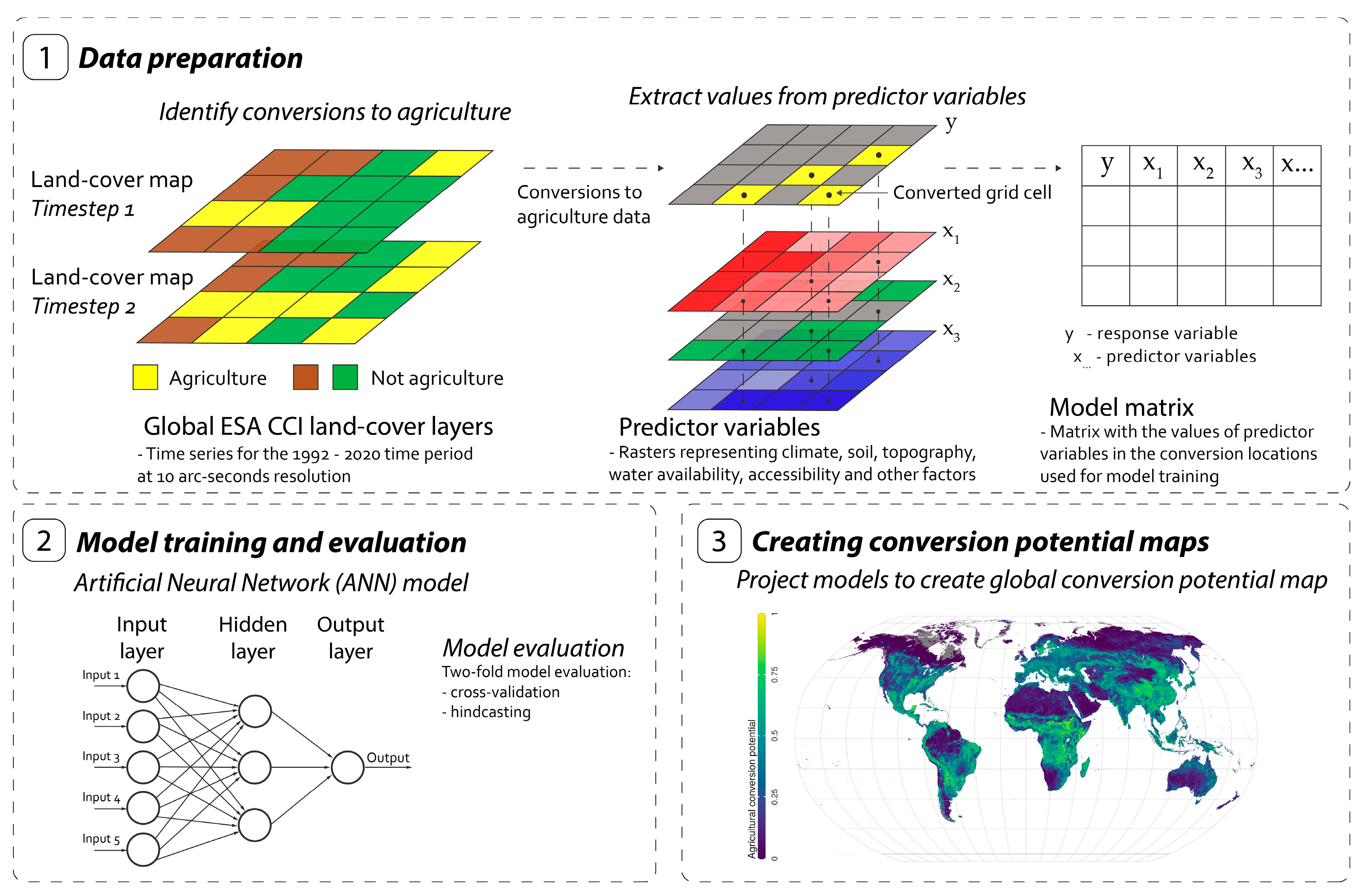
2.1. General Approach

Our approach for producing the global agricultural conversion potential maps consisted of three main steps (Figure 1). In the first step, we identified locations of conversions to agricultural land from 2007 to 2020 and collected data on possible predictors of conversion. In the second step, we used the data on agricultural conversions and corresponding predictor variables to train artificial neural network (ANN) models, which we validated using both cross-validation and hindcasting. For the hindcasting, we used conversions to agricultural land observed from 1992 to 2006. Finally, we combined the validated ANN models with global raster layers of the predictor variables to create global maps of agricultural expansion potential.

2.2. Identifying Locations of Agricultural Conversion

We identified locations of agricultural conversion based on the ESA CCI land-cover dataset. This dataset contains yearly global land-cover maps based on remotely sensed data for 1992–2020 [20,21]. The dataset has a spatial resolution of 10 arc-seconds (approximately 300 m at the equator) and includes 22 main land-cover categories. Agricultural land encompasses rainfed crops (ESA CCI class 10), irrigated crops (ESA CCI class 20), and two types of mosaic cropland: mosaics of >50% cropland with <50% natural vegetation (ESA CCI class 30) and mosaics of >50% natural vegetation with <50% cropland (ESA CCI class 40). Because irrigated and rainfed crops are not consistently distinguished as separate categories in all regions of the world, we combined rainfed and irrigated crops into a single category of ‘cropland only’. Thus, we distinguished three agricultural land categories: cropland only (71% of the total agricultural area in the ESA CCI dataset), mosaics with >50% crops (15% of the total agricultural area), and mosaics with <50% crops (14% of the total agricultural area). We divided the dataset in two parts, selecting the years 2007–2020 for training our agricultural conversion potential model and the 1992–2006 period for model evaluation (hindcasting). For each of the three agricultural land categories and each of the two periods, we extracted the locations of conversion as those where the land cover changed into the respective agricultural land categories.

2.3. Predictor Variables

We selected a set of predictor variables that are expected to influence the spatial patterns of conversion into agricultural land [15,19,22,23,24]. These variables are related to the topographic characteristics of the landscape, climate properties, soil properties, accessibility, and previous land cover (Table 1). As topographic landscape properties, we included elevation, terrain slope, northness (a measure of terrain aspect), and the topographic wetness index (TWI). We retrieved elevation from the global MERIT Digital Elevation Model (DEM) [25] and calculated terrain slope and northness from this same DEM using the gdaldem function from the Geospatial Data Abstraction Library (GDAL) 2.2.2 software [26]. We obtained the TWI from ISRIC’s worldgrids database (https://web.archive.org/web/20170620003114/http://www.worldgrids.org/doku.php/wiki:twisre3; accessed on 24 February 2023). As climatic predictors, we included annual mean values of temperature and precipitation as well as their seasonality (standard deviation and coefficient of variation of monthly values, respectively), as both are expected to influence local suitability for crop production [15,24]. We retrieved the climatic predictor variables based on long-term mean monthly values over 1979–2013 as provided by the CHELSA climate database [27]. Soil-related predictors included the available water capacity, cation exchange capacity, soil pH, and the organic carbon, clay, silt, and sand contents. We retrieved these variables from the SoilGrids database, using geometric mean values across 0–30 cm depth profiles [28]. We further included four variables indicative of the accessibility of a site: the distance to roads, distance to urban areas, distance to existing croplands, and the presence of protected areas. We calculated the distances to roads, urban areas, and agriculture as the Euclidean distance to any of the road types I–IV in the GRIP global road dataset [29] and cells classified as urban or agricultural in the ESA CCI land-cover map for 2007, respectively. We obtained a layer with protected areas from the World Database of Protected Areas [30]. Finally, we included the human population density (year 2000) from the Gridded Population of the World database [31] and variables that describe the land-cover category that was present in a given location prior to the conversion into agriculture to account for land-cover inertia, i.e., how easy or difficult it is to convert current land cover into agriculture (Table 1).
The original spatial resolution of the predictor variables ranged from 90 to 1000 m (Table 1). We resampled all predictor variables to a spatial resolution of 10 arc-seconds (300 m) to match the spatial resolution of the land-cover maps. We resampled variables with a higher spatial resolution by calculating the average value of cells within the larger 10 arc-second cell. We resampled variables with a lower spatial resolution to 10 arc-seconds using cubic spline resampling, which produces smoother surfaces compared with simpler resampling techniques [32]. To harmonize the spatial resolution and extent of the predictor variables, we used GDAL 2.2.2.

2.4. Training the ANNs

We modelled the potential of conversion into each of the three agricultural land categories as a function of the predictor variables using artificial neural network (ANN) models, which are known for their ability to learn and mimic complex phenomena [33,34]. We employed feed-forward ANNs with a single hidden layer, i.e., a layer of mathematical functions to translate the input data (predictor variables) into the output (conversion potential). Prior to training the ANNs, we selected grid cells not being converted into cropland from 2007 to 2020 as reference or absence locations. To avoid pseudo-replication, we performed spatial subsampling or thinning of the data by randomly selecting one observation (either a conversion or non-conversion) per 1 km2 grid cell (i.e., the spatial resolution of the coarsest predictor variables; see Table 1). For each agricultural land category, we then randomly selected a number of non-conversions equal to the number of conversions in order to obtain a balanced sample. We further log-transformed predictor variables with clear positive skew (human population density and distance variables) in order to limit the effect of extreme values, and we standardized all continuous predictor variables, as recommended for ANN training [35].
To prevent overfitting of the model, we tuned the hyperparameters that control the number of units in the hidden layer and the weights decay regularization function by identifying the combination that returned the highest kappa value in cross-validation. To this end, we performed 10-fold cross-validation with two-thirds of the data used for model training and the remaining third for model assessment. The tuning resulted in 20 units in the hidden layer and a decay value of 0.001, hence we used these values for training the final ANN models. For model training and hyperparameter tuning, we used the R packages caret version 6.0-81 [36] and nnet version 7.3-12 [37].

2.5. Model Evaluation

We evaluated the predictive performance of the ANN models based on both cross-validation and hindcasting. For the cross-validation, we used two-thirds of the 2007–2020 data for model training and the remaining third to evaluate the models. For the hindcasting, we used the data from the 1992–2006 period to evaluate the models that were trained on the full dataset for 2007–2020. We evaluated the performance of the models using the area under the curve of the receiver operator characteristic (AUC in short). The AUC metric ranges between 0 and 1, where a value of 1 indicates perfect discrimination between presence and absence (in our case, conversion or non-conversion to agricultural land) [38]. In addition, we evaluated the relationships between the conversion potential and the predictor variables. First, we estimated the relative importance of each variable for predicting the conversion potential of each of the three cropland categories. To that end, we followed a variable permutation procedure similar to the random forest variable importance algorithm [38], using our ANN model trained on the full 2007–2020 dataset. We used this model to make predictions of the conversion potential with permuted values for the predictor variable of concern, correlated those predictions with the predictions of the model based on the original (non-permuted) data, and quantified the variable importance as one minus the Pearson’s correlation coefficient (r). Thus, the higher the correlation between the predictions based on the data with the permuted variable and the predictions based on the original data, the less important the permuted variable. We repeated this procedure 100 times for each of the predictor variables to obtain an importance measure and corresponding standard error for each. Second, we assessed the direction and magnitude of changes in conversion potential in relation to each of the predictor variables by establishing partial dependence plots (PDPs). PDPs show how a response variable changes in relation to a variable of interest given average predictions over all the other predictor variables. We created the PDPs using R package pdp version 0.7.0 [39].

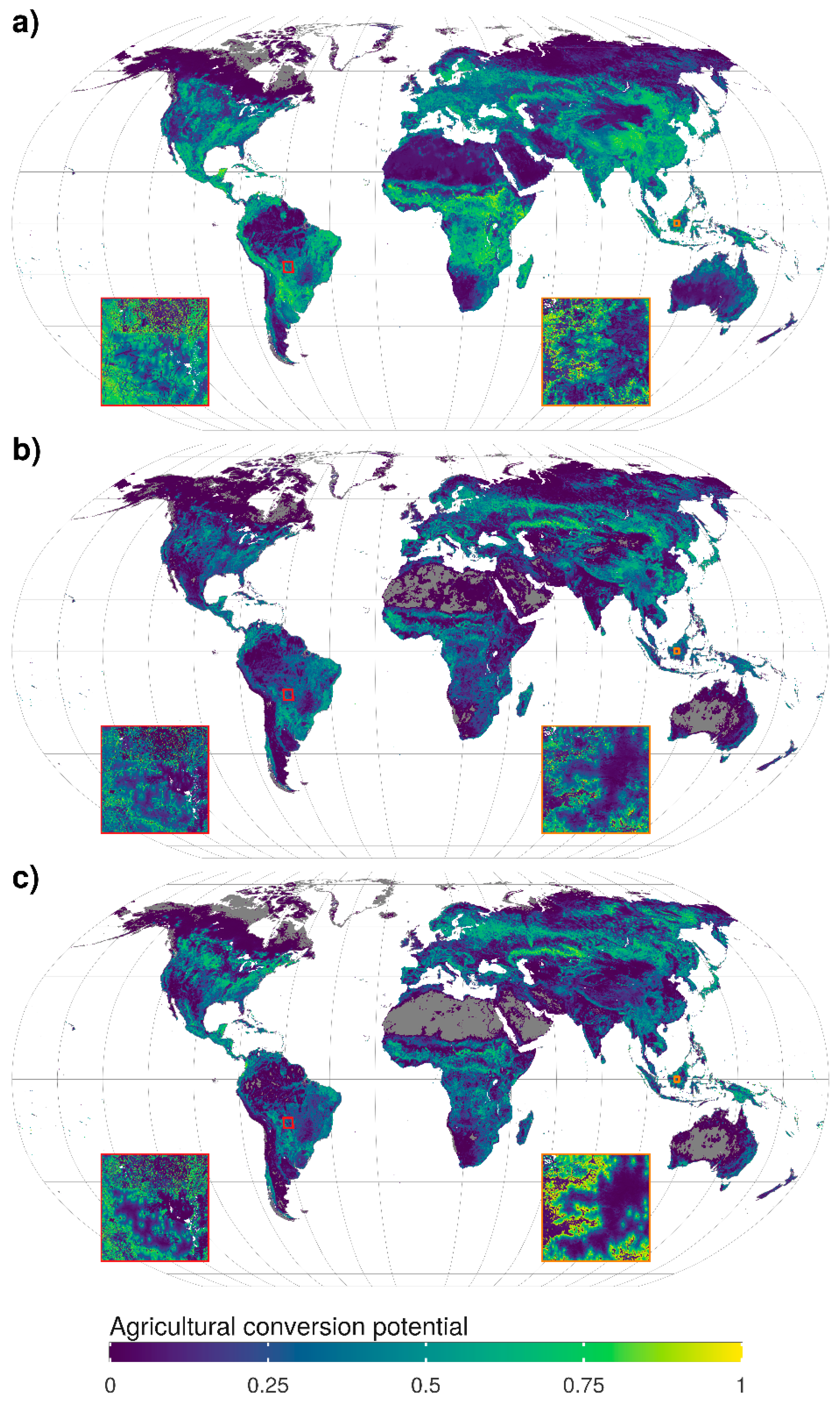
2.6. Conversion Potential Maps

After training and evaluating the ANN models, we applied them to create global maps of agricultural conversion potential for each of the three cropland categories. Because this process is highly computationally intensive, we divided the globe into 6630 tiles of equal size. We cropped the predictor variable rasters for each tile and then used the trained ANN models to obtain predictions for each tile by splitting the task across multiple cluster computing nodes. Afterwards, we merged the resulting conversion potential maps across the tiles into global maps (Figure 1). For splitting and merging of the layers we used GDAL version 2.2.2. In addition to the 10 arc-seconds layers, we provide layers of 30 arc-seconds and 5 arc-minutes resolutions for more coarse-grained applications. We provide three layers for each aggregated set, containing the minimum, mean, and maximum values of the 10 arc-seconds values within the larger cells. All conversion potential maps are publicly available for download from https://doi.org/10.5281/zenodo.7665902 (accessed on 24 February 2023). We performed all modelling and post-processing in the R environment (version 3.6.3). Scripts are available via GitHub at https://github.com/MirzaCengic/agriculture_suitability (accessed on 24 February 2023).

3. Results

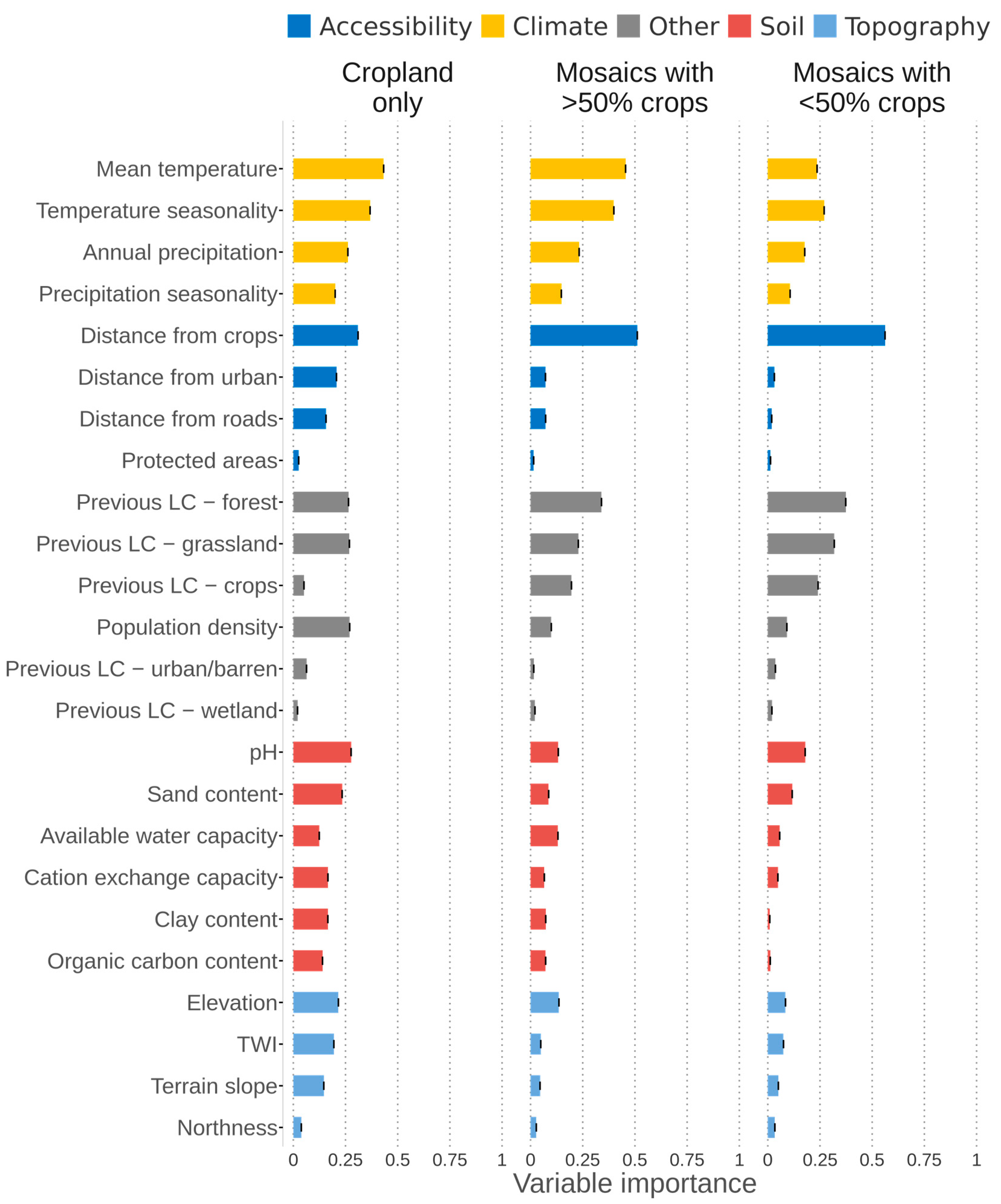
3.1. Model Performance

The performance evaluation of the ANN models revealed AUC values of 0.88–0.93 in the cross-validation and 0.83–0.91 in the hindcasting (Table 2). The high AUC values indicate that the models are well able to distinguish locations of agricultural conversions from locations without conversion. Further, the high model performance in hindcasting indicates that the predictors of agricultural conversion patterns and the magnitude of their influence have remained relatively constant over the past decades.

3.2. Conversion Potential Maps

Our global agricultural conversion potential maps revealed high conversion probabilities in some of the tropical regions (Congo basin, Borneo, New Guinea, Amazon region), the Cerrado and Chaco regions in South America, the North American plains, eastern China, the northern parts of the Indian sub-continent, and the steppes of Kazakhstan and southern Russia (Figure 2). Although the conversion potential maps revealed considerable similarities between the three cropland categories, we also found a few differences. For example, for the cropland only category, we found high conversion potential particularly in the tropical regions, whereas for the mosaic categories, the steppes of Kazakhstan and southern Russia stood out (Figure 2).

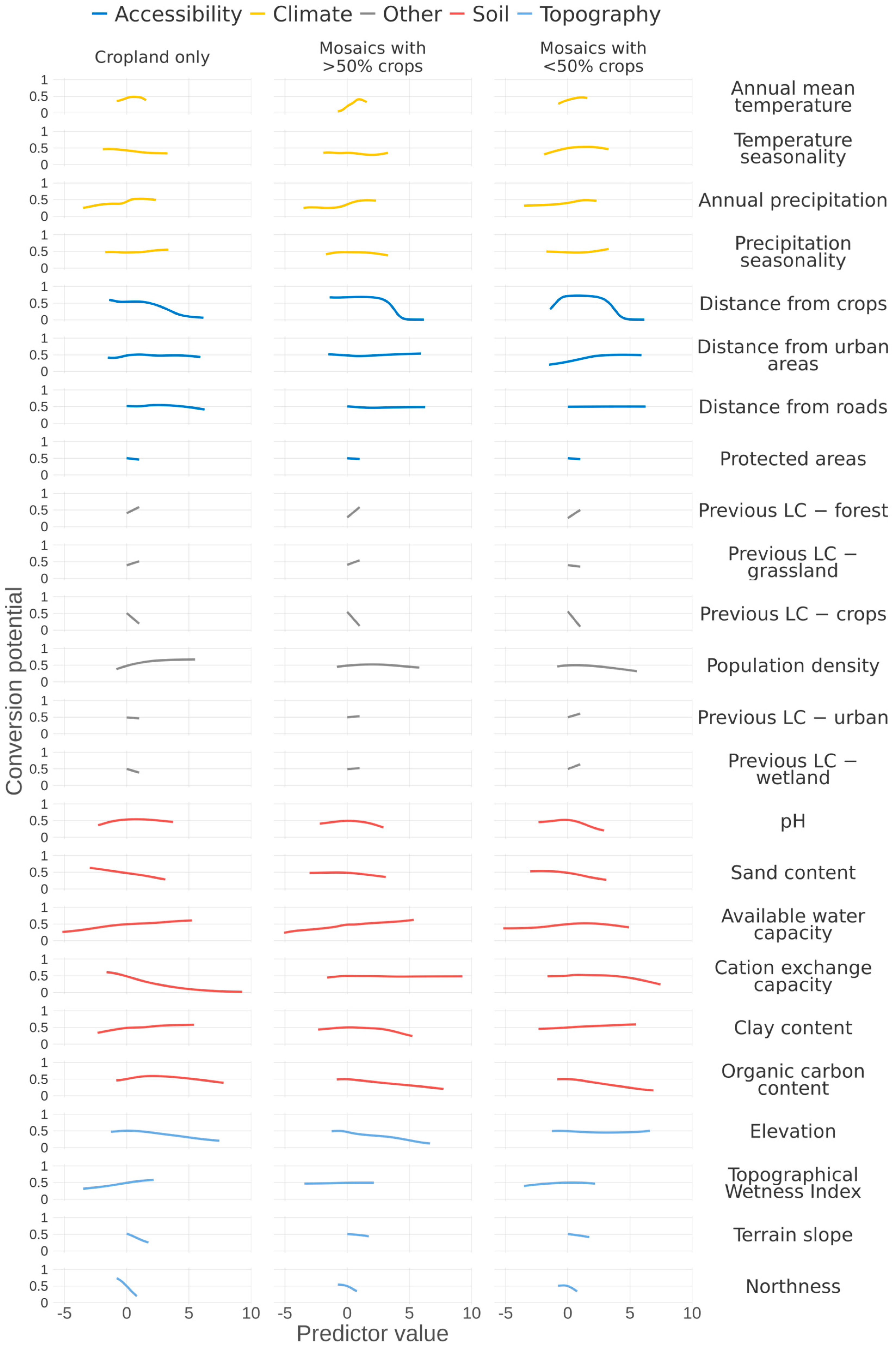
3.3. Relationships between Conversion Potential and Predictor Variables

Important predictors of conversion potential included climatic variables (mainly mean annual temperature and seasonality, followed by annual precipitation) and the distance from existing cropland (Figure 3). For mean annual temperature, we found unimodal responses, with increases in conversion potential followed by declines at higher annual mean temperature values (Figure 4). The relationship between conversion potential and temperature seasonality was negative for cropland only and mosaics with >50% crops and positive for mosaics with <50% crops, indicating that conversion to the latter is more prevalent in more variable climatic conditions. For all three cropland categories, we found positive relationships between conversion potential and annual precipitation. The distance to existing cropland was especially important for the mosaic categories (Figure 3). For mosaics with >50% crops as well as croplands only, we found a monotonic decrease in conversion potential with increasing distance from existing cropland. For mosaics with <50% crops, we observed a slightly different response, with the highest conversion potential at some distance from the existing cropland (Figure 4). Of the variables representing previous land cover, forest was relatively important. Here, we found positive response relationships across the three cropland categories, indicating that recent conversions have been relatively prevalent in forested areas. Of the soil variables, pH was relatively important, with the highest conversion potential at average pH values (Figure 4).

4. Discussion

To our knowledge, this study is the first to derive global agricultural conversion potential maps based on recent past conversions rather than current land-use patterns and at a considerably improved spatial resolution compared with existing global land change models. These improvements were possible thanks to the development and release of the ESA CCI dataset, which offers a consistent time series of global land-cover maps. The ANN models that we developed to establish the agricultural conversion potential maps showed high performance not only in cross-validation (2007–2020) but also in hindcasting (1992–2006). This reflects that the frontiers of agricultural expansion have been relatively stable during the past decades, with agricultural expansion happening mainly in regions where some expansion has already occurred [19]. In line with this, we found that the proximity to existing cropland was indeed a main predictor of conversion potential across all three agricultural land categories (Figure 3 and Figure 4). The clustered expansion of cropland, in turn, may reflect that agricultural expansion frontiers build on agglomeration economies, where the clustering of related firms and organizations brings benefits such as increased access to knowledge, a pooled labour market, lower transportation costs, and reduced entry barriers [40].
Our conversion potential maps revealed various hotspots of conversion that coincide with regions of large recent agricultural expansion [8]. For example, the Chaco and Cerrado regions in South America are characterized by significant recent expansions of large-scale soy bean cultivation [41], whereas the Congo basin is home to various countries with substantial expansions of oil palm plantations [42]. Large oil palm plantation expansions have also occurred in Sumatra and Borneo over the recent decades [43]. The high conversion potential in the steppes in Kazakhstan and southern Russia may reflect the recultivation of land that was abandoned after the collapse of the former Soviet Union [44]. However, our maps show relatively high conversion probabilities also in regions without significant recent increases in total agricultural land area, such as North America, or even with net declines in agricultural land, such as western Europe [8]. In these regions, the rates of expansion might be similar to or even lower than the rates of abandonment, which in turn may reflect that the expansion of large farms goes alongside the abandonment of smallholder farms [45].
The high performance of our ANN models in both cross-validation and hindcasting indicates that our conversion potential maps can help to improve the projections of global land change models provided that the drivers underlying the global patterns of agricultural expansion remain the same. As such, our conversion potential maps are useful for researchers and practitioners interested in assessing the locations and effects of future agricultural expansion, for example in integrated assessment modelling or biodiversity impact modelling [9,18]. To that end, our maps need to be combined with estimates of the expected future demands for agricultural land per socioeconomic region. In such a coupled approach, our global conversion potential maps can be used to spatially allocate the additional agricultural land demands. In this context, it is important to note that the modelled relationships between the agricultural conversions and our set of predictors may result in non-zero probabilities also in areas that are highly unlikely to be converted into agriculture, such as urban areas or strictly protected nature reserves. This implies that users of our maps may need to implement an additional map layer that masks areas unavailable for agricultural expansion. We also stress that our maps represent agricultural conversion potential conditional on the predictor variables that we included, implying that our maps do not capture the possible influences of other potentially relevant predictors. For example, our conversion potential models and maps do not account for permafrost, which may pose significant challenges to possible agricultural expansion at higher latitudes in response to climate change [46].
Finally, we note that our mapping procedure based on a consistent time series of land-cover maps is easily extended to other land-use or land-cover types, such as built-up areas. The procedure can also be applied to obtain maps representing the potential of agricultural abandonment, which is characterized by its own dynamics and specific drivers [45]. Ultimately, a consistent set of conversion potential maps for multiple land categories, combined with corresponding estimates of demands per socioeconomic region, may result in more accurate and spatially detailed projections of land change, including potential shifts in agricultural land. This in turn would be an asset, in particular, for assessments of changes in ecological patterns and processes that operate on small scales [18].

5. Conclusions

We produced global maps of agricultural conversion potential at a 10 arc-seconds resolution (about 300 m), based on location-specific information of sites where land was converted into agriculture in the recent past (2007–2020). We obtained these maps with machine learning models that we tested with two complementary approaches (cross-validation and hindcasting). The testing revealed a good model performance (AUC > 0.80), indicating that the resulting maps can be used to project future agricultural expansion over the coming decades, provided that the drivers underlying the global spatial patterns of expansion remain the same. Integrating our maps into scenario-based land use and integrated assessment modelling can help to better quantify impacts of future agricultural expansion on ecosystems and, ultimately, lead to more informed policy decisions. Further, our modelling workflow can be extended to other land-use types and with the development and improvement of long-term time series data, enable more accurate assessment of drivers and patterns of land change and its effects.

Author Contributions

M.A.J.H. conceived the initial idea. M.Č., Z.J.N.S., A.M.S. and M.A.J.H. designed the study. M.Č. carried out the data processing and analysis. M.Č. and A.M.S. wrote the paper. All authors contributed to refining the methodology, interpreting the results, and improving the manuscript. All authors have read and agreed to the published version of the manuscript.

Funding

MČ: ZJNS, PD, JCD, CL, ES, and AMS were supported by PBL Netherlands Environmental Assessment Agency via the GLOBIO project (www.globio.info (accessed on 24 February 2023)). MAJH was supported by the project 016.Vici.170.190, which was financed by The Netherlands Organisation for Scientific Research (NWO).

Data Availability Statement

All the modelling and post-processing were performed in the R environment (version 3.6.2). Scripts are available via GitHub at https://github.com/MirzaCengic/agriculture_suitability (accessed on 24 February 2023). The conversion potential maps are publicly available for download from https://doi.org/10.5281/zenodo.7665902 (accessed on 24 February 2023). In addition to the 10 arc-seconds layers, we provide layers of 30 arc-seconds and 5 arc-minutes and 10 arc-minutes resolutions for more coarse-grained applications. We provide four layers for each aggregated set, containing the minimum, mean, median and maximum values of the 10 arc-seconds values within the larger cells.

Conflicts of Interest

The authors declare that they have no conflict of interest.

References

  1. Ellis, E.C.; Goldewijk, K.K.; Siebert, S.; Lightman, D.; Ramankutty, N. Anthropogenic transformation of the biomes, 1700 to 2000. Glob. Ecol. Biogeogr. 2010, 19, 589–606. [Google Scholar] [CrossRef]
  2. Lambin, E.F.; Meyfroidt, P. Global land use change, economic globalization, and the looming land scarcity. Proc. Natl. Acad. Sci. USA 2011, 108, 3465–3472. [Google Scholar] [CrossRef] [PubMed] [Green Version]
  3. Turner, B.L.; Lambin, E.F.; Reenberg, A. The emergence of land change science for global environmental change and sustainability. Proc. Natl. Acad. Sci. USA 2007, 104, 20666–20671. [Google Scholar] [CrossRef] [Green Version]
  4. Laurance, W.F.; Sayer, J.; Cassman, K.G. Agricultural expansion and its impacts on tropical nature. Trends Ecol. Evol. 2014, 29, 107–116. [Google Scholar] [CrossRef] [PubMed]
  5. Kuipers, K.J.J.; Hilbers, J.P.; Garcia-Ulloa, J.; Graae, B.J.; May, R.; Verones, F.; Huijbregts, M.A.J.; Schipper, A.M. Habitat fragmentation amplifies threats from habitat loss to mammal diversity across the world’s terrestrial ecoregions. One Earth 2021, 4, 1505–1513. [Google Scholar] [CrossRef]
  6. Houghton, R.A.; House, J.I.; Pongratz, J.; van der Werf, G.R.; DeFries, R.S.; Hansen, M.C.; Le Quere, C.; Ramankutty, N. Carbon emissions from land use and land-cover change. Biogeosciences 2012, 9, 5125–5142. [Google Scholar] [CrossRef] [Green Version]
  7. Suh, S.; Johnson, J.A.; Tambjerg, L.; Sim, S.; Broeckx-Smith, S.; Reyes, W.; Chaplin-Kramer, R. Closing yield gap is crucial to avoid potential surge in global carbon emissions. Glob. Environ. Change-Hum. Policy Dimens. 2020, 63, 102100. [Google Scholar] [CrossRef]
  8. Li, W.; MacBean, N.; Ciais, P.; Defourny, P.; Lamarche, C.; Bontemps, S.; Houghton, R.A.; Peng, S.S. Gross and net land cover changes in the main plant functional types derived from the annual ESA CCI land cover maps (1992–2015). Earth Syst. Sci. Data 2018, 10, 219–234. [Google Scholar] [CrossRef] [Green Version]
  9. Doelman, J.C.; Stehfest, E.; Tabeau, A.; van Meijl, H.; Lassaletta, L.; Gernaat, D.; Hermans, K.; Harmsen, M.; Daioglou, V.; Biemans, H.; et al. Exploring SSP land-use dynamics using the IMAGE model: Regional and gridded scenarios of land-use change and land-based climate change mitigation. Glob. Environ. Change-Hum. Policy Dimens. 2018, 48, 119–135. [Google Scholar] [CrossRef] [Green Version]
  10. Alexander, P.; Prestele, R.; Verburg, P.H.; Arneth, A.; Baranzelli, C.; Silva, F.B.E.; Brown, C.; Butler, A.; Calvin, K.; Dendoncker, N.; et al. Assessing uncertainties in land cover projections. Glob. Change Biol. 2017, 23, 767–781. [Google Scholar] [CrossRef] [Green Version]
  11. Meiyappan, P.; Dalton, M.; O’Neill, B.C.; Jain, A.K. Spatial modeling of agricultural land use change at global scale. Ecol. Model. 2014, 291, 152–174. [Google Scholar] [CrossRef] [Green Version]
  12. Seto, K.C.; Guneralp, B.; Hutyra, L.R. Global forecasts of urban expansion to 2030 and direct impacts on biodiversity and carbon pools. Proc. Natl. Acad. Sci. USA 2012, 109, 16083–16088. [Google Scholar] [CrossRef] [PubMed] [Green Version]
  13. Van Asselen, S.; Verburg, P.H. Land cover change or land-use intensification: Simulating land system change with a global-scale land change model. Glob. Change Biol. 2013, 19, 3648–3667. [Google Scholar] [CrossRef] [PubMed]
  14. Eitelberg, D.A.; van Vliet, J.; Verburg, P.H. A review of global potentially available cropland estimates and their consequences for model-based assessments. Glob. Change Biol. 2015, 21, 1236–1248. [Google Scholar] [CrossRef]
  15. van Asselen, S.; Verburg, P.H. A Land System representation for global assessments and land-use modeling. Glob. Change Biol. 2012, 18, 3125–3148. [Google Scholar] [CrossRef] [Green Version]
  16. Hasegawa, T.; Fujimori, S.; Ito, A.; Takahashi, K.; Masui, T. Global land-use allocation model linked to an integrated assessment model. Sci. Total Environ. 2017, 580, 787–796. [Google Scholar] [CrossRef] [Green Version]
  17. Hoskins, A.J.; Bush, A.; Gilmore, J.; Harwood, T.; Hudson, L.N.; Ware, C.; Williams, K.J.; Ferrier, S. Downscaling land-use data to provide global 30 ‘‘estimates of five land-use classes. Ecol. Evol. 2016, 6, 3040–3055. [Google Scholar] [CrossRef] [Green Version]
  18. Schipper, A.M.; Hilbers, J.P.; Meijer, J.R.; Antao, L.H.; Benitez-Lopez, A.; de Jonge, M.M.J.; Leemans, L.H.; Scheper, E.; Alkemade, R.; Doelman, J.C.; et al. Projecting terrestrial biodiversity intactness with GLOBIO 4. Glob. Change Biol. 2020, 26, 760–771. [Google Scholar] [CrossRef] [Green Version]
  19. Eigenbrod, F.; Beckmann, M.; Dunnett, S.; Graham, L.; Holland, R.A.; Meyfroidt, P.; Seppelt, R.; Song, X.P.; Spake, R.; Vaclavik, T.; et al. Identifying agricultural frontiers for modeling global cropland expansion. One Earth 2020, 3, 504–514. [Google Scholar] [CrossRef]
  20. Defourny, P.; Kirches, G.; Brockmann, C.; Boettcher, M.; Peters, M.; Bontemps, S.; Lamarche, C.; Schlerf, M.; Santoro, M. Land Cover CCI Product User Guide Version 2.0; UCL Geomatics: Leuven, Belgium, 2017. [Google Scholar]
  21. Defourny, P.; Lamarche, C.; Marissiaux, Q.; Brockmann, C.; Boettcher, M.; Kirches, G. Product User Guide and Specification. ICDR Land Cover 2016-2020; European Centre for Medium-Range Weather Forecasts (ECMWF): Reading, UK, 2021. [Google Scholar]
  22. Amatulli, G.; Domisch, S.; Tuanmu, M.N.; Parmentier, B.; Ranipeta, A.; Malczyk, J.; Jetz, W. A suite of global, cross-scale topographic variables for environmental and biodiversity modeling. Sci. Data 2018, 5, 180040. [Google Scholar] [CrossRef] [Green Version]
  23. Sacks, W.J.; Deryng, D.; Foley, J.A.; Ramankutty, N. Crop planting dates: An analysis of global patterns. Glob. Ecol. Biogeogr. 2010, 19, 607–620. [Google Scholar] [CrossRef]
  24. Wheeler, T.R.; Craufurd, P.Q.; Ellis, R.H.; Porter, J.R.; Prasad, P.V.V. Temperature variability and the yield of annual crops. Agric. Ecosyst. Environ. 2000, 82, 159–167. [Google Scholar] [CrossRef]
  25. Yamazaki, D.; Ikeshima, D.; Tawatari, R.; Yamaguchi, T.; O’Loughlin, F.; Neal, J.C.; Sampson, C.C.; Kanae, S.; Bates, P.D. A high-accuracy map of global terrain elevations. Geophys. Res. Lett. 2017, 44, 5844–5853. [Google Scholar] [CrossRef] [Green Version]
  26. GDAL/OGR Contributors. GDAL/OGR Geospatial Data Abstraction Software Library; Version 2.2.2; Open Source Geospatial Foundation: Chicago, IL, USA, 2020. [Google Scholar]
  27. Karger, D.N.; Conrad, O.; Bohner, J.; Kawohl, T.; Kreft, H.; Soria-Auza, R.W.; Zimmermann, N.E.; Linder, H.P.; Kessler, M. Climatologies at high resolution for the earth’s land surface areas. Sci. Data 2017, 4, 170122. [Google Scholar] [CrossRef] [PubMed] [Green Version]
  28. Hengl, T.; de Jesus, J.M.; Heuvelink, G.B.M.; Gonzalez, M.R.; Kilibarda, M.; Blagotic, A.; Shangguan, W.; Wright, M.N.; Geng, X.Y.; Bauer-Marschallinger, B.; et al. SoilGrids250m: Global gridded soil information based on machine learning. PLoS ONE 2017, 12, e0169748. [Google Scholar] [CrossRef] [PubMed] [Green Version]
  29. Meijer, J.R.; Huijbregts, M.A.J.; Schotten, K.; Schipper, A.M. Global patterns of current and future road infrastructure. Environ. Res. Lett. 2018, 13, 064006. [Google Scholar] [CrossRef] [Green Version]
  30. UNEP-WCMC and IUCN. Protected Planet: The World Database on Protected Areas (WDPA). 2017. Available online: http://www.protectedplanet.net/ (accessed on 24 February 2023).
  31. Center for International Earth Science Information Network (CIESIN). Gridded Population of the World, Version 4 (GPWv4). 2016. Available online: https://sedac.ciesin.columbia.edu/data/collection/gpw-v4 (accessed on 24 February 2023).
  32. Li, J.; Heap, A.D. Spatial interpolation methods applied in the environmental sciences: A review. Environ. Model. Softw. 2014, 53, 173–189. [Google Scholar] [CrossRef]
  33. Basse, R.M.; Omrani, H.; Charif, O.; Gerber, P.; Bodis, K. Land use changes modelling using advanced methods: Cellular automata and artificial neural networks. The spatial and explicit representation of land cover dynamics at the cross-border region scale. Appl. Geogr. 2014, 53, 160–171. [Google Scholar] [CrossRef]
  34. Barbarossa, V.; Huijbregts, M.A.J.; Beusen, A.H.W.; Beck, H.E.; King, H.; Schipper, A.M. FLO1K, global maps of mean, maximum and minimum annual streamflow at 1 km resolution from 1960 through 2015. Sci. Data 2018, 5, 180052. [Google Scholar] [CrossRef] [Green Version]
  35. Haykins, S.S. Neural Networks and Learning Machines; Pearson Education: Upper Saddle River, NJ, USA, 2009. [Google Scholar]
  36. Kuhn, M. Building predictive models in R using the caret package. J. Stat. Softw. 2008, 28, 1–26. [Google Scholar] [CrossRef] [Green Version]
  37. Venables, W.N.; Ripley, B.D. Modern Applied Statistics with S.; Springer: New York, NY, USA, 2002. [Google Scholar]
  38. Swets, J.A. Measuring the accuracy of diagnostic systems. Science 1988, 240, 1285–1293. [Google Scholar] [CrossRef] [PubMed] [Green Version]
  39. Greenwell, B.M. pdp: An R Package for Constructing Partial Dependence Plots. R J. 2017, 9, 421–436. [Google Scholar] [CrossRef] [Green Version]
  40. Garrett, R.D.; Lambin, E.F.; Naylor, R.L. The new economic geography of land use change: Supply chain configurations and land use in the Brazilian Amazon. Land Use Policy 2013, 34, 265–275. [Google Scholar] [CrossRef]
  41. Graesser, J.; Ramankutty, N.; Coomes, O.T. Increasing expansion of large-scale crop production onto deforested land in sub-Andean South America. Environ. Res. Lett. 2018, 13, 084021. [Google Scholar] [CrossRef] [Green Version]
  42. Ordway, E.M.; Asner, G.P.; Lambin, E.F. Deforestation risk due to commodity crop expansion in sub-Saharan Africa. Environ. Res. Lett. 2017, 12, 044015. [Google Scholar] [CrossRef]
  43. Carlson, K.M.; Curran, L.M.; Ratnasari, D.; Pittman, A.M.; Soares, B.S.; Asner, G.P.; Trigg, S.N.; Gaveau, D.A.; Lawrence, D.; Rodrigues, H.O. Committed carbon emissions, deforestation, and community land conversion from oil palm plantation expansion in West Kalimantan, Indonesia. Proc. Natl. Acad. Sci. USA 2012, 109, 7559–7564. [Google Scholar] [CrossRef] [PubMed] [Green Version]
  44. Meyfroidt, P.; Schierhorn, F.; Prishchepov, A.V.; Muller, D.; Kuemmerle, T. Drivers, constraints and trade-offs associated with recultivating abandoned cropland in Russia, Ukraine and Kazakhstan. Glob. Environ. Change-Hum. Policy Dimens. 2016, 37, 1–15. [Google Scholar] [CrossRef]
  45. Hatna, E.; Bakker, M.M. Abandonment and expansion of arable land in Europe. Ecosystems 2011, 14, 720–731. [Google Scholar] [CrossRef] [Green Version]
  46. Jones, M.K.W.; Schwoerer, T.; Gannon, G.M.; Jones, B.M.; Kanevskiy, M.Z.; Sutton, I.; St Pierre, B.; St Pierre, C.; Russell, J.; Russell, D. Climate-driven expansion of northern agriculture must consider permafrost. Nat. Clim. Change 2022, 12, 699–703. [Google Scholar] [CrossRef]
Figure 1. Schematic overview of the agricultural conversion potential modelling procedure according to three main steps: (1) data preparation: identification of locations of conversions to agriculture and extraction of predictor variables, (2) training and evaluating the ANN models, and (3) applying the trained models to create global maps of agricultural conversion potential.
Land 12 00579 g001
Figure 2. Global conversion potential maps for the three agricultural categories: (a) cropland only, (b) mosaics with >50% crops, and (c) mosaics with <50% crops. For visualization purposes, the global maps were resampled to a spatial resolution of 5 arc-minutes (~10 km) and displayed in Robinson projection. Areas with probabilities close to zero (1‰ cut-off value) are shown in grey. Inset maps are displayed at the original 10 arc-seconds resolution.
Land 12 00579 g002
Figure 3. Importance of the predictor variables for the conversion potential into three categories of agricultural land: cropland only (left), mosaics with >50% crops (centre), and mosaics with <50% crops (right). Bars and error bars represent the means and standard errors based on 100 repetitions of the variable importance estimation procedure. LC = land cover; TWI = topographic wetness index.
Land 12 00579 g003
Figure 4. Partial dependence plots showing the change in conversion potential in relation to each of the predictors (standardized values) for cropland only (left), mosaics with >50% crops (centre), and mosaics with <50% crops (right).
Land 12 00579 g004
Table 1. List of predictor variables with original units and spatial resolution (prior to resampling and standardization).
VariableUnitSpatial ResolutionSource
ClimateAnnual mean temperature°C1 kmCHELSA Climate [27]
Temperature seasonality°C1 kmCHELSA Climate [27]
Annual precipitationmm/year1 kmCHELSA Climate [27]
Precipitation seasonalitydimensionless1 kmCHELSA Climate [27]
SoilAvailable water capacity%250 mSoilGrids [28]
Cation exchange capacitycmol/kg250 mSoilGrids [28]
Clay content%250 mSoilGrids [28]
Organic carbon contentg/kg250 mSoilGrids [28]
pHdimensionless250 mSoilGrids [28]
Silt content%250 mSoilGrids [28]
Sand content %250 mSoilGrids [28]
TopographyElevationm90 mMERIT DEM [25]
Slopedegrees90 mthis study
Northness indexdimensionless90 mthis study
Topographic Wetness Index (TWI)dimensionless250 mISRIC worldgrids
AccessibilityDistance to roadsm300 mGRIP [29]
Distance to agriculturem300 mthis study
Protected areas0 or 1300 mWDPA [30]
Distance to urban areasm300 mthis study
OtherPopulation densitypersons/km21 kmGPW [31]
Previous land cover * (agriculture, forests, grasslands, wetlands, urban/barren)0 or 1300 mthis study
* Previous land cover includes five binary layers with aggregated land-cover categories, indicating whether in the year prior to the conversion the land cover belonged to the given land-cover type or not. Agriculture encompasses rainfed, irrigated, and mosaic croplands; forests encompass all categories with tree cover; grasslands encompass shrublands, grasslands, and sparse vegetation; wetlands include flooded forests with brackish or saline water; urban/barren includes urban areas, bare areas, and permanent snow and ice.
Table 2. Model performance as measured by the area under the curve of the receiver operator characteristic (AUC), shown for three categories of agricultural land and two evaluation procedures. For the cross-validation, we used two-thirds of the 2007–2020 data to train the models and the remaining third for evaluation. Hindcasted models were trained on the entire dataset containing the conversions from 2007 to 2020 and evaluated on a dataset from the preceding period (1992–2006).
Agricultural CategoryAUC
Cross-validationHindcasting
Cropland only0.880.84
Mosaics with >50% crops0.930.91
Mosaics with <50% crops0.930.83
Disclaimer/Publisher’s Note: The statements, opinions and data contained in all publications are solely those of the individual author(s) and contributor(s) and not of MDPI and/or the editor(s). MDPI and/or the editor(s) disclaim responsibility for any injury to people or property resulting from any ideas, methods, instructions or products referred to in the content.

