Article

Early Evidence That Soil Dryness Causes Widespread Decline in Grassland Productivity in China

1
Henan Normal University, Xinxiang 453007, China
2
Ministry of Education Key Laboratory for Western Arid Region Grassland Resources and Ecology, Xinjiang Agricultural University, Urumqi 830000, China
3
Ministry of Education Key Laboratory for Biodiversity Science and Ecological Engineering, Fudan University, Shanghai 200438, China
4
Lanzhou University, Lanzhou 730020, China
5
College of Resources and Environment, Northwest A&F University, Yangling 712100, China
6
Key Research Insititute of Yellow River Civilization and Sustainable Development Collaborative Innovation Center on Yellow River Civilization, Henan University, Kaifeng 475001, China
7
College of Resources and Environmental Sciences, China Agricultural University, Beijing 100193, China
*
Author to whom correspondence should be addressed.
Land 2023, 12(2), 484; https://doi.org/10.3390/land12020484
Submission received: 9 January 2023 / Revised: 1 February 2023 / Accepted: 2 February 2023 / Published: 15 February 2023

Abstract

:
The burning of fossil fuels by humans emits large amounts of CO2 into the atmosphere and strongly affects the Earth’s carbon balance, with grassland ecosystems changing from weak carbon sinks that were previously close to equilibrium to core carbon sinks. Chinese grasslands are located in typical arid–semi-arid and semi-arid climatic regions, and drought events in the soil and atmosphere can have strong and irreversible consequences on the function and structure of Chinese grassland ecosystems. Based on this, we investigated the response of the gross primary production (GPP) of Chinese grasslands to land–atmosphere moisture constraints, using GPP data simulated through four terrestrial ecosystem models and introduced copula functions and Bayesian equations. The main results were as follows: (1) Soil moisture trends were not significant, and changes were dominated by interannual variability. The detrended warm-season SM correlated with GPP at 0.48 and 0.63 for the historical and future periods, respectively; thus, soil moisture is the critical water stress that regulates interannual variability in Chinese grassland GPP. (2) The positive correlation between shallow SM (0–50 cm) and GPP was higher (r = 0.62). Shallow-soil moisture is the main soil layer that constrains GPP, and the soil moisture decrease in shallow layers is much more likely to cause GPP decline in Chinese grasslands than that in deep-soil water. (3) The probability of GPP decline in Chinese grasslands caused by drought in shallow soils of 0–20 and 20–50 cm is 32.49% and 27.64%, respectively, which is much higher than the probability of GPP decline in deeper soils. In particular, soil drought was more detrimental to grassland GPP in Xinjiang and the Loess Plateau. (4) The probability of soil drought causing GPP decline was higher than that of atmospheric drought during the historical period (1.78–8.19%), but the probability of an atmospheric drought-induced GPP deficit increases significantly in the future and becomes a key factor inhibiting GPP accumulation in some regions (e.g., the Loess Plateau). Our study highlighted the response of grassland ecosystems after the occurrence of soil drought, especially for the shallow-soil-water indicator, which provides important theoretical references for grassland drought disaster emergency prevention and policy formulation.

1. Introduction

Global climate change has fundamentally altered the inherent patterns of variability of weather phenomena, such as precipitation and temperature, leading to the increasing frequency of extreme weather events such as droughts, heat waves, and cold waves [1]. Extreme events severely affect the composition and function of terrestrial ecosystems, thus affecting the terrestrial carbon cycle and its feedback to the climate system. Extreme droughts, in particular, are highly anticipated natural disasters because they occur with the highest frequency and exert the greatest influence [2,3]. The intensity and frequency of droughts are the most limiting factors affecting terrestrial vegetation growth and carbon cycling [4], and droughts reduce the water available to vegetation directly [5], with extensive and profound effects on carbon uptake in terrestrial ecosystems [6].
Recent research pointed out that terrestrial carbon sinks are often strongly influenced by interannual fluctuations in terrestrial water storage. Terrestrial water constraints are also an important limiting factor for the accumulation of ecosystem gross primary productivity (GPP) [7], that is, the largest carbon flux [8]. However, the terrestrial water storage referred to by previous studies includes all water types, such as soil water, groundwater, surface water, and canopy water. In contrast, there is a lack of exploration of the possible effects of water shortage from the soil on ecosystem productivity, as the terrestrial water variability is considerably sensitive [9]. Soil moisture accounts for a relatively large proportion of terrestrial water storage [10,11]. However, soil moisture is a generalized concept, and it is generally loosely considered as all the water within 3 m below the ground surface. Considering the differences in terrestrial water adaptation of different plants and the strong link between water availability to grass plants and root depth [12], it is necessary to explore the varying effects of soil water constraints at different soil depths on ecosystem GPP.
In addition to soil drought, atmospheric drought has been recently reported as one of the hydraulic processes that affect ecosystem productivity [13]. Plants initially draw water from the soil for photosynthesis and simultaneously dissipate it in the atmosphere through transpiration from plant leaves [14]. Both supply and depletion stresses can significantly reduce terrestrial carbon uptake and crop yields [6] and cause widespread vegetation mortality. However, current research on the primacy of soil moisture (SM) and atmospheric moisture (vapor pressure difference, VPD) on ecosystem productivity response is controversial. Novick et al. (2016) pointed out that VPD has a greater constraining effect on stomatal conductance and evapotranspiration than SM, which is more important for carbon accumulation. Moreover, as atmospheric VPD will continue to rise in the future, the negative effect of VPD on stomatal conductance during the plant growing season will increase significantly, as will its dominance on carbon fixation [15]. Liu et al. (2020) proposed the opposite conclusion and claimed that soil drought is the main stress that threatens GPP accumulation in more than 70% of regional ecosystems worldwide, and by decoupling SM–VPD, found that the impact of VPD on terrestrial ecosystems is much smaller than that of soil moisture [16]. Given the complexity of the coupling between VPD and SM, it is highly desirable to use novel methods (e.g., probabilistic) to compare the dominance of VPD and SM on ecosystem GPP.
Chinese grasslands are mainly distributed in arid and semi-arid regions (typical temperate grasslands and montane grasslands) and the Tibetan Plateau (typical alpine grasslands), where the ecological environment is fragile [17,18], providing a natural barrier to ecological security in Central and Western China. Due to the unique arid–semi-arid environment and distinct vertical zonality, the carbon cycling processes in Chinese grassland ecosystems are very sensitive to climate change and human disturbances [19,20,21]. In this study, Chinese grasslands were the study area, and copula functions and Bayesian equations were introduced to explore the conditional probability of GPP decline in Chinese grassland ecosystems when atmospheric drought (high-VPD event) and soil drought (low-SM event) occurred, respectively. We aim to address the following three issues.
(1)
To analyze the interannual variability of SM and GPP in Chinese grasslands and to explore the mechanisms of SM regulation of GPP in Chinese grassland ecosystems during historical and future periods.
(2)
To compare the correlation between the effects of SM on ecosystem GPP in different soil layers, and analyze the conditional probability of drought in soils of different soil layers causing a decline in GPP in Chinese grasslands.
(3)
To calculate the difference between the probability of ecosystem loss due to soil drought minus the probability of ecosystem loss due to atmospheric drought and determine the key moisture constraints controlling GPP in Chinese grasslands.

2. Materials and Methods

2.1. Materials

2.1.1. GPP Datasets

We used the model outputs from four global vegetation dynamics models (CARAIB, LPJ GUESS, LPJmL, ORCHIDEE DGVM) as GPP (monthly, 0.5°) products. The model GPP products are all derived from the harmonized general circulation model IPSL-CM5A-LR as meteorological forcing data, considering historical (1901–2005) and further (2006–2099) scenarios. The results of the model simulations of GPP are all implemented strictly in accordance with the ISIMIP 2b standard protocol, so differences between model outputs are only related to the complexity of the model. Considering that a single model only provides valuable and usable insights at the regional scale, to effectively eliminate intra-model variability and reduce uncertainty in GPP products, we conducted pooled averaging of multi-model GPPs for further processing. Since only LPJmL of the four models of ISIMIP 2b provides mainstream high-emission RCP8.5 climate projections, the future scenarios consider only medium to high GHG emission scenarios (RCP6.0).

2.1.2. SM Datasets

SM data were used to characterize the degree of soil drought. The previous comparison of individual simulated values and pooled averages shows that the amplitudes of the pooled averages are much smaller than those of individual simulated values [22]. In other words, the ensemble averaging method can effectively eliminate the effect of variability within the model, which can effectively reduce the uncertainty between different models. Therefore, we selected the pooled average soil moisture products from the four model outputs.
However, it should be additionally noted that the different models differ in their simulation of land atmospheric exchange fluxes and carbon- and water-cycle stocks in natural and agro-ecosystems, so each model provides different soil moisture soil thicknesses. Here, to match soil layer thickness and reduce data errors, the soil moisture counted was limited to the sum of the moisture in all soil layers within 3 m below ground.
In addition, to explore the binding effect of soil moisture in different soil layers on ecosystem GPP, the LPJmL model with explicit soil stratification thickness was extracted for further analysis. The LPJmL model output included soil moisture at different soil depths of 0–20 cm, 20–50 cm, 50–100 cm, 100–200 cm, and 200–300 cm.

2.1.3. VPD Datasets

We also obtained standard-corrected model input parameters (temperature and relative humidity) from ISIMIP to calculate VPD, which refers to the difference between saturated vapor pressure and actual vapor pressure (AVP) at a given temperature and is a direct measure of the intensity of atmospheric drought [23].
V P D = S V P - A V P
Saturated vapor pressure is a non-linear function of atmospheric temperature and can be obtained directly from atmospheric temperature calculations with the following empirical formula:
S V P = 6.112 × f a × e 17.67 T a T a + 243.5
f a = 1 + 7 × 10 - 4 + 3.46 × 10 - 6 P m s t
P m s t = P m s l T a + 273.16 T a + 273.16 + 0.0065 × Z
where Ta is the atmospheric surface temperature (°C); Z is the altitude (m); Pmsl is the atmospheric pressure at mean sea level (≈1013.25 hPa); and Pmst is the atmospheric pressure (hPa).
A V P = R H 100 × S V P
The above equation shows that warming significantly increases the amount of water vapor held by the atmosphere at saturation (saturation vapor pressure), while the actual vapor pressure of the atmosphere (depending on the relative humidity) remains relatively constant. Consequently, the warming is followed by a non-linear increase in VPD.

2.1.4. Definition of Warm Season and Screening for Warm-Season GPP, SM, and VPD

The warm season in the grid cell was defined as the hottest three month average (one value per year) given that the warm season coincides with the main growing season of plants [24].
We adopted the previous idea of averaging (one value per year) GPP, SM, and VPD for the three months with larger mean temperature values, as carbon loss due to moisture shortage is often most intense in the hottest three months. Therefore, the location of the three months with the largest temperature on the grid unit was extracted by counting the monthly mean temperatures over the period 1901–2005, and the mean GPP, SM, and VPD for the three months with the largest temperature on the metric scale were then filtered from the time series for analysis.

2.2. Methods

2.2.1. Interannual Correlation Measures

For extreme value theory, the correlation coefficient is a good indicator and is commonly used to measure the effect of dependence on the likelihood of binary extreme values [24]. We calculated the interannual correlation between the SM and GPP model dataset per pixel. To remove the influence of climate change signals on long-term trends, we performed a linear detrending of the bivariate prior to calculating correlations.
Commonly used correlations include Pearson and Spearman [25]. Pearson correlation coefficients are only applicable to correlation analyses where the two variables are linear; however, the effect of SM on GPP is often non-linear. Therefore, we chose the Spearman’s rank correlation coefficient to analyze the correlation between SM and GPP, with a stronger negative correlation between the two variables indicating more significant negative feedback.

2.2.2. Bivariate Linkage to Calculate the Probability of Conditions under Soil (or Atmospheric) Drought Conditions

Based on the copula function and Bayesian equation, we drew on the novel probabilistic assessment framework constructed by Wang et al. (2021) and He et al. (2022) to calculate the conditional probability of a simultaneous soil drought (or atmospheric drought) scenario. This consists of the following three steps:
(1) Fitting of marginal distributions
Bivariate frequency analysis requires that the distributions of the random variables U and V be determined, so determining the marginal distribution of the bivariate is a prerequisite for constructing the joint probability distribution. We used a non-parametric method for fitting the marginal distributions, because non-parametric estimation methods do not require prior estimation or assumptions about all parameters of the copula function of the dependence structure between the bivariate variables, and can be directly estimated to obtain the fitted values at any point [26]. Non-parametric kernel density estimation is therefore more widely used in practice than conventional parameter estimation (e.g., normal, gamma), and can effectively eliminate errors in the fitted joint probability distribution due to partial singular values. Kernel density estimation is the most widely used test in the field of non-parametric estimation [27], where the kernel distribution produces a non-parametric probability density estimate that adapts itself to the data, rather than selecting a probability density estimate with a particular parameter. Here, we used kernel density estimation to derive marginal distribution fits for the bivariate.
The kernel function density estimation method is described by the following equation:
f n x = 1 n h i = 1 n K x - x i h
fn(x) represents the kernel density value; n represents the number of samples in the bandwidth range; h is the window or bandwidth, representing a reasonable smoothing parameter and h > 0; K is the kernel smoothing function; (xxi) is the distance between points to xi; and x1, x2, … xn are random samples from an unknown distribution.
The kernel density estimate of the cumulative distribution function is described as follows:
F n x = - x f n t d t = 1 n i = 1 n G x - x i h , G x = - x K t d t
(2) Fitting and optimization of joint probability distributions
Copulas are multivariate distribution functions defined in the domain of [0, 1] and are used to describe correlations between multiple variables. The bivariate copula function is commonly used to describe the dependence structure between two sets of random variables and to count the joint probability of an event (such as a compound drought) occurring. Sklar confirms that the copula function is unique in that if F(·,·) is a joint distribution function and X(·) and Y(·) are marginal distribution functions of independent variables, then there must be a copula function C(·,·), satisfying
F x , y = C X , Y
When X(·) and Y(·) are continuous, there must be a uniquely determined C. Conversely, X(·) and Y(·) are only one-dimensional distribution functions.
According to Sklar’s theorem, the joint probability distribution function FX,Y(x, y) for variables X and Y can be expressed as:
F X , Y x , y = C F X x , F Y y = P X x , Y y
where Fx(x) = P(Xx) and Fy(y) = P(Yy) are the cumulative distribution functions of the variables X (e.g., SM) and Y (e.g., GPP). C is the joint distribution function of U = Fx(x) and V = Fy(y) after marginal fitting, and the new sequence U and V after the marginal distribution fitting transformation has the characteristics of a uniform distribution.
In addition, a binary copula family connection function is required to calculate the joint probability of an event, and we chose the joint distribution functions Clayton, Frank, Gumbel, t, and Gaussian copula to describe the possible dependency structure of the two variables. The function expression is described in Table 1.
The copula family linkage function was used to reconstruct the dependence structure of the bivariate. To more accurately describe the dependence structure of the bivariate, the best-fitting distribution function was then selected from the five mentioned above for further analysis. The goodness-of-fit test is based on the minimized squared Euclidean distance (SED) and is described as follows:
S E D = C U V / C 2
where CUV is the empirical value of the individual binary copula function fit and C is the theoretical value.
(3) Bayesian formula modeling conditional probabilities
Bayesian formulas are causal imputations related to a priori probabilities and phenomenal probabilities (observed objective probabilities) and are a deformation of conditional probabilities. The descriptive formula is:
P A | B = P A P B | A P B = P A B P B , P B 0
where P(B) is the probability of the occurrence of event B (a priori probability); P(AB) is derived from step 2 and represents the probability of simultaneous occurrence of event A and event B. By simple reasoning, we know that to determine the conditional probability of the occurrence of loss of ecosystem GPP under drought stress conditions, we need to calculate the probability of the occurrence of drought and the probability of the co-occurrence of increased drought and decreased productivity, where P(AB) can be interpreted as the compound probability of the simultaneous occurrence of drought and loss of vegetation productivity.
P(A|B) represents the probability of event A occurring if event B is known to occur (conditional probability); in other words, P(−GPP > 90%|VPD > 90%) can be interpreted as the probability of occurrence of −GPP above 90% when VPD is above 90%. The specific formula is described as follows:
P - G P P > 90 % | V P D > 90 % = 1 - P - G P P > 90 % - P V P D > 90 % + C - G P P > 90 % , V P D > 90 % 1 - P V P D > 90 %
Note that it takes a threshold above a certain value of atmospheric VPD to initiate a decline in ecosystem GPP, so we used −GPP to calculate the conditional probability in the bivariate relationship. Here, the conditional probability of P(−GPP > 90%|VPD > 90%) is identical to that of P(GPP < 10%|VPD > 90%). Therefore, above equation can be interpreted as the conditional probability of an event occurring with a GPP below 10% in the case of VPD above 90%. It is expressed as follows:
P G P P < 10 % | V P D > 90 % = 1 - P G P P < 10 % - P V P D > 90 % + C G P P < 10 % , V P D > 90 % 1 - P V P D > 90 %
We used percentages to define the degree of atmospheric drought and the degree of ecosystem GPP deficit, defining all samples with VPD values above 90%, 70%, and 50% as severe, moderate, and mild atmospheric drought and all samples with GPP values below 10%, 30%, and 50% as severe, moderate, and mild vegetation deficit.
Unlike atmospheric drought, a soil drought event can only be recognized as occurring when soil moisture falls below a certain threshold. We focused on the joint probability of extreme SM (below 10%, 30%, 50%) and GPP (below 10%, 30%, 50%). Thus, the conditional probability of a decline in ecosystem GPP in the presence of an extreme soil drought event can be derived by combining the Bayes’ equation described as:
P G P P < 10 % | S M < 10 % = C G P P < 10 % , S M < 10 % P S M < 10 %
Similarly to atmospheric drought, we defined severe, moderate, and mild soil drought for all samples with SM values below 10%, 30%, and 50%.

3. Results

3.1. Characteristics of Long-Term Changes in Chinese Grassland SM and Its Constraints on Ecosystem GPP

Th long-term trend of soil moisture simulation in Chinese grasslands is not insignificant over the past 100 years. The annual SM in the historical period had an insignificant soil-degenerating aridity trend, and future projections were largely constant (Figure 1a). The warm-season SM showed a similar trend, but the moisture anomaly domain was significantly higher in the warm season than in the annual (Figure 1b). Compared to the trends, the interannual variability of soil moisture in Chinese grasslands is highly significant, as can be seen in periods such as 1930–1950 and 2050–2060 when soil moisture is significantly higher. In conclusion, the long-term change of soil moisture is mainly controlled by its interannual fluctuations. Therefore, the next analysis will focus on the regulation of the interannual variability of soil moisture on ecosystem GPP.
Figure 2 shows that the interannual variability of SM and GPP is similar, i.e., years with low SM correspond to low GPP, and the two are strongly positively correlated. The correlations between SMIAV and GPPIAV are 0.171 and 0.477 for the whole year in the historical and future periods, respectively, and the fluctuation patterns of both are found to have been basically consistent since 1950. The degree of correlation was significantly stronger in the warm season than in the whole year, with correlations of 0.48 and 0.63 between them year by year for the historical and future periods, respectively, and both passed the significance level (p < 0.05) test. We concluded that soil moisture is an important factor that strongly regulates ecosystem GPP, and when soil moisture is below a certain threshold, it significantly constrains the accumulation of ecosystem GPP, because an insufficient soil moisture supply significantly forces a decrease in plant photosynthetic capacity, which in turn leads to a decrease in ecosystem GPP. Moreover, this effect more strongly restricts plant growth during the growing season.
Next, the correlations of SMIAV and GPPIAV were calculated using a sliding window of 41 years for the whole year and warm season from 1901 to 2099 (Figure 3). The bivariate correlations were found to be consistently positive in most periods and regions of Chinese grasslands, and the correlation values were higher for the warm season than for the whole year. The correlations between SMIAV and GPPIAV in Mongolia, the Loess Plateau, and Xinjiang all exceeded 0.4 and passed the significance test, while the correlation in the Tibetan Plateau grasslands gradually increased to 0.2 from year to year. This reflects that the regulation of GPP by soil moisture is always positive, i.e., it suppresses plant growth in water-scarce years and promotes it in water-abundant years. In comparison, the positive correlations in the warm season are higher in all regions and stages than in the whole year, and the correlations in Chinese grasslands are always around 0.4 throughout the year, while the correlations in the warm season have been over 0.5 since 1970. In the Xinjiang and Loess Plateau regions in particular, the correlations of the warm-season bivariate exceeded 0.6. This indicated that the regulation of GPP by soil moisture is higher in the warm season than in the whole year; in other words, the warm-season soil moisture deficit can trigger more serious ecosystem GPP loss events in most cases. Given that our study discusses the effect of soil moisture constraint events on ecosystem GPP, the choice of warm-season bivariate better reflects the limiting effect of extreme moisture constraints on carbon uptake in grasslands, and, therefore, the SM and GPP in the warm season were chosen for further analysis.

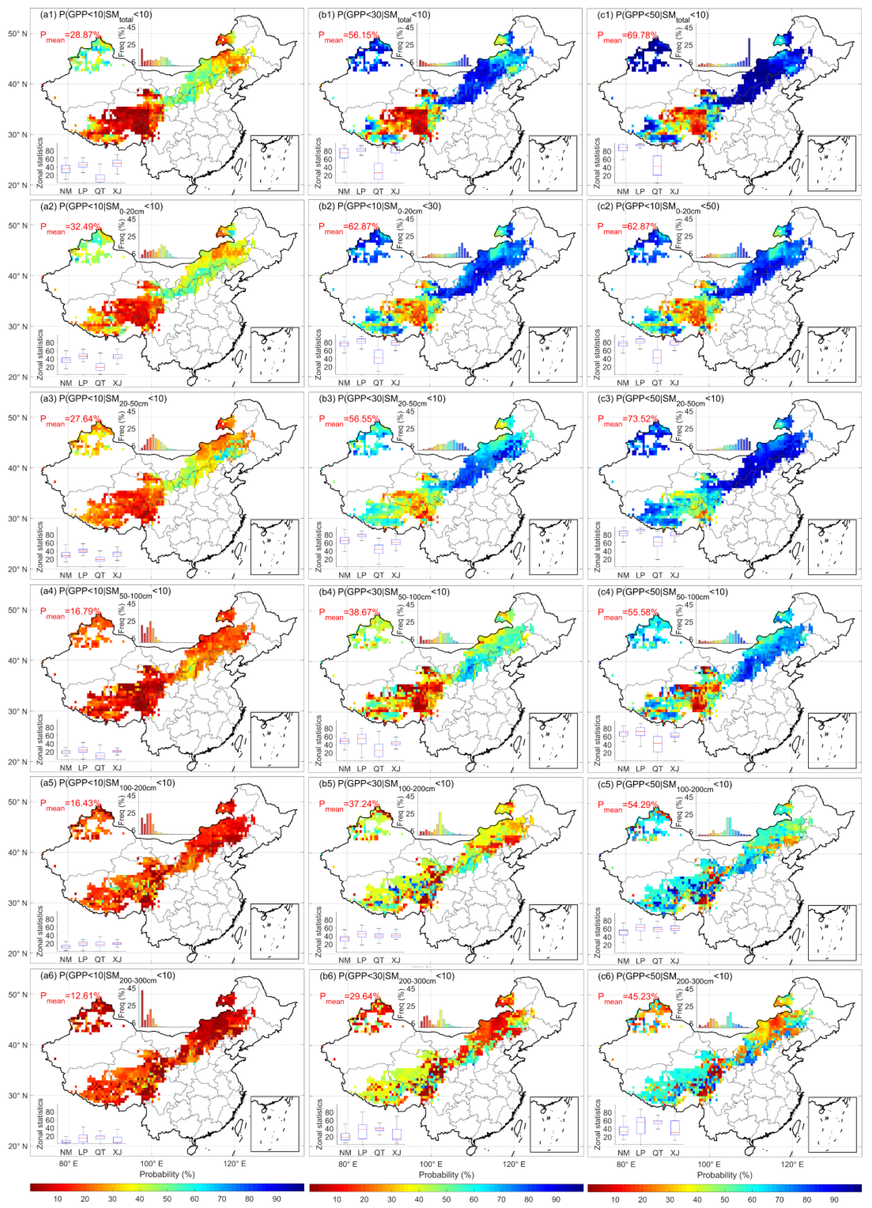
3.2. Comparison of the Regulation of GPP by Different Soil Layers

The impact on the GPP of the ecosystem varies across soil layers due to differences in rainwater recharge and evapotranspiration at different depths. The warm-season SM and GPP were correlated at the meta-scale to compare the bivariate structure between SM and GPP at different soil depths (Figure 4). The bivariate correlations for shallow soils (0–20 and 20–50 cm) were found to show significant interannual agreement, with highly significant positive correlations in both historical and future periods. Deeper soils (100–200 and 200–300 cm) with higher possible difficulty in water use for plants, did not show a significant consistent interannual correlation in the historical period, and the interannual relationship between the two variables tended to be consistent in the future period. As shown in Figure 4c, most of the pixel correlations between shallow-soil water and GPP are greater than 0, implying a strong positive coupling between the two, with shallow-soil water deficit significantly constraining the accumulation of GPP in the ecosystem. In contrast, about half of the pixels of the deep-soil water are on both sides of the 0 value line, showing very high uncertainty in the regulation of GPP. Overall, the correlation between ecosystem GPP and the SM of different soil layers showed a higher correlation the closer to the surface the soil layer was. Comparing different soil layers, it can be seen that soil moisture at different depths has an inconsistent regulating effect on ecosystem GPP, and uncertainty has a non-negligible effect on GPP constraint.
Figure 5 shows the spatial distribution of the probability of different degrees of ecosystem GPP loss under the precondition of extreme drought in soils with different soil moisture levels, and found that the probabilities show great differences between different soil levels. The probability of severe GPP loss induced by drought events at the 0–20 cm soil depth was as high as 32.49%, decreasing to 27.64%, 16.79%, 16.43%, 16.43%, and 12.61% with the increase in soil depth. We found that after drought in shallow soils, the ecosystem GPP tended to be severely deficient due to water limitations, while the probability of drought-induced vegetation deficit in deep soils was lower. In addition, we also emphasized that the probability of severe shallow-soil drought induced moderate and mild ecosystem GPP loss, while the ecosystem GPP was significantly higher than that of deep-soil drought.
The locations of the spatial distribution of ecosystem GPP loss probabilities for severe, moderate, and mild were basically the same, indicating that soil drought events of different soil depths had weaker effects on the changes in probability at different locations. The spatial heterogeneity of ecosystem GPP loss induced by shallow-soil drought events was stronger. Xinjiang and the Loess Plateau are the most susceptible grasslands to soil drought, followed by Inner Mongolia grasslands and Tibetan Plateau grasslands being the least affected. The probabilities associated with deep-soil drought were more uniform and consistent in space, with less variation among regions (Figure 5(a6)).

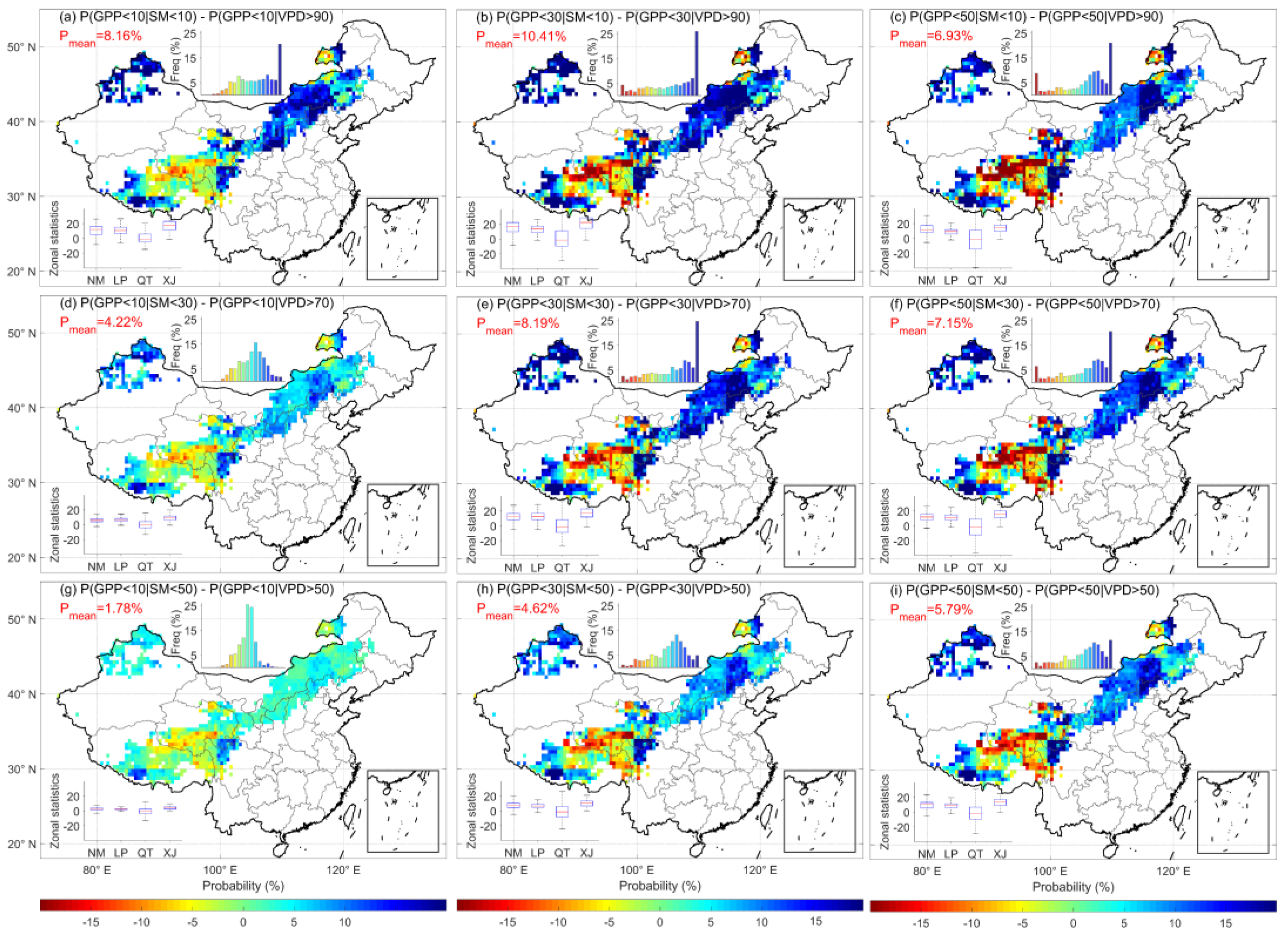
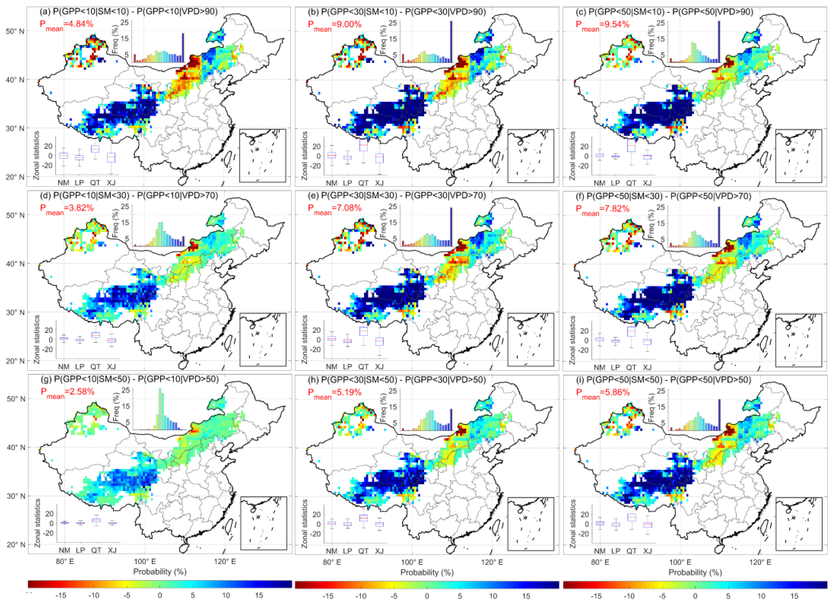
3.3. Comparison of the Probability of High-VPD and Low-SM Events Leading to Ecosystem GPP Deficits

The difference was obtained by subtracting the probability of GPP decline due to soil drought from the probability of GPP decline due to atmospheric drought, which can be used to compare the primary and secondary effects of soil drought and atmospheric drought on the constraint of ecosystem GPP. A positive value represents a stronger constraint of soil drought on GPP, while a negative value represents a stronger constraint of atmospheric drought. For the historical period, we found that soil drought in Chinese grasslands causes a higher probability of ecosystem GPP loss than atmospheric drought, but the results vary widely with different threshold settings (Figure 6). The difference between the two was relatively large in the most severe drought scenario, with 8.16%, 10.41%, and 6.93% differences for severe, moderate, and mild ecosystem GPP losses, respectively (Figure 6a–c). The differences also showed different degrees of reduction with decreasing drought levels. From the probability perspective, we concluded that the overall impact of soil drought on Chinese grassland ecosystems is significantly higher than that of atmospheric drought, and the probability of GPP deficit caused by soil drought is on average 1–10% higher than atmospheric drought. However, the difference was found to be spatially heterogeneous, with soil drought in Inner Mongolia, the Tibetan Plateau, and the Loess Plateau apparently causing a higher probability of ecosystem GPP loss, which is the main constraint limiting GPP accumulation. In contrast, the probability of atmospheric drought causing ecosystem GPP deficit was higher in the grassland of the Tibetan Plateau, which represents a stronger constraint of atmospheric drought on the GPP of the Tibetan Plateau.
For the future period, soil drought remains the main water constraint limiting the accumulation of GPP in the ecosystem (Figure 7). However, compared to the historical period, the spatial differences changed significantly. The difference in the Loess Plateau tends to be negative from the positive value in the historical period, indicating that atmospheric drought will become the most important moisture constraint in the future. Inner Mongolia and Xinjiang, although still positive, have decreased compared with the historical period, indicating that the moisture constraint from the atmosphere has increased and the soil moisture constraint has weakened. The Tibetan Plateau is very unique, and soil drought will become the main constraint on GPP accumulation in the Tibetan Plateau ecosystem in the future, and its probability difference is more than 10%.

4. Discussion

4.1. Soil Moisture More Strongly Regulates Carbon Balance Than Atmospheric Indicators in Chinese Grasslands

Terrestrial ecosystem models can obtain high-resolution long time series of soil moisture products, bridging the gap between remote sensing and station observations [22] and providing important information for exploring long-term soil drought evolution. We confirmed that soil moisture deficit can severely weaken the accumulation of ecosystem GPP and is an important aspect in regulating the interannual dynamics of GPP. Previous studies have shown that CO2 growth rates are sensitive to observed changes in terrestrial moisture, i.e., drought years are associated with rapid increases in atmospheric CO2 [7]; higher water availability promotes ecosystem productivity fixation, and water loss attenuates it [28,29]. Our results are similar and showed that low SM corresponds to low GPP, reflecting a reduced potential for ecosystem CO2 uptake in years with low soil water. Thus, a lack of soil water supply would affect the division and expansion of individual plant cells and greatly reduce the ability to obtain carbon from the atmosphere, which in turn would result in a decrease in ecosystem GPP.
Considering that soil water content is closely related to precipitation, most of the precipitation infiltrates into the soil, except for a small portion that evaporates and is trapped by the canopy [30]. Most of the water available for plant uptake originates from precipitation, which affects the photosynthetic capacity of plants and is mainly regulated by the intra-annual distribution of precipitation and differences in precipitation intensity [31]. Changes in the intra-annual distribution of precipitation can lead to a mismatch between water availability and plant growth requirements [32]. For example, precipitation events that occur during the germination period do not match actual water demand and supply. As a result, much of the water is likely to be inefficient and ‘wasted’ in the evapotranspiration process [33]. It has been suggested that increasing precipitation early in the growing season can have a positive impact on semi-arid grassland productivity [34]. This may be due to a number of factors, including the fact that the earlier the precipitation, the higher the soil moisture, and the fact that more precipitation early in the growing season promotes plant root growth. In contrast, more precipitation events later in the growing season do not significantly improve photosynthetic capacity or carbon accumulation [35]. In addition, changes in the magnitude or intensity of precipitation events can alter the vertical distribution of soil moisture, which is closely linked to the underground activity of plants [36]. Small precipitation events tend to increase the shallow-soil water content and stimulate shallow-rooted plant activity (photosynthesis and autotrophic respiration) and soil microbial activity. Large precipitation events are more effective at replenishing deep-soil water content, which may be more effective in triggering deep plant activity [37].
We keenly captured the extremely close coupling between Chinese grassland productivity and soil moisture, with soil moisture surplus and deficit directly regulating the direction of ecosystem carbon revenues and expenditures. Precipitation is the most direct source of replenishment for soils [38], and precipitation surplus and deficit can be considered to regulate productivity in Chinese grasslands. However, given that soil moisture is the main source of water directly available to plants, this study innovatively used soil moisture as the main water constraint to analyze its relative influence on GPP.

4.2. Soil Moisture Is a Key Water Constraint Controlling the Grassland Productivity in China

Previous studies have found that soil drought is the dominant constraint on drought stress in most ecosystems worldwide [16]. We have confirmed that soil drought is indeed the main water constraint threatening GPP in Chinese grassland ecosystems from a probabilistic perspective. However, we noted that the probability difference between soil drought and atmospheric drought causing an ecosystem GPP deficit gradually decreases or reverses to a negative value in most regions in the future. This represents a clear increase in the extent to which atmospheric drought will affect ecosystems in the future and a decrease in the importance of soil drought in dominating vegetation deficits. This is likely due to the fact that atmospheric VPD has increased rapidly over the past century and will remain the growing trend in the future (Supplementary Figure S1), while soil moisture trends have remained stable over time (Figure 1). Continued atmospheric constraints force ecosystems to adapt to water stress by closing stomata or stopping plant growth due to the inability to coordinate water–carbon fluxes [39]. We found that the future scenario for the Tibetan Plateau is one in which the temperature limitation of alpine ecosystems is lifted by rising temperatures, possibly due to increased atmospheric pressure that promotes vegetation growth rather than inhibiting it, thus causing soil drought to remain the main moisture constraint limiting GPP accumulation in the Tibetan Plateau in the future. It is important that identifying the primary and secondary moisture constraints from the soil and atmosphere remains a challenge [40], and a probabilistic perspective provides only a possibility rather than a definitive conclusion. In the future, there is a need for further clarification of this long-standing and complex issue to open up new avenues for improved modeling and better management of drought risk.
However, the interannual regulation of ecosystem GPP was significantly different for soil moisture at different soil depths. We found that shallow-soil water (0–50 cm) was the dominant soil layer regulating interannual variability in GPP, probably because the most accessible water to grassland plants comes from shallow soils and is the direct source [41]. In water-scarce weather, most plants preferentially draw water from the soil [12], and roots easily take up residual water from shallow soils in a variety of ways, including mass flow, diffusion, and interception [42]. Only when shallow-soil water is exhausted can deep-rooted plants draw water from deeper soils [43]. We also confirmed that the probability of ecosystem GPP loss induced by water deficit in shallow soils is much higher than that of deep-soil water, representing a greater dependence on shallow-soil water for plant growth, and that negative anomalies in shallow-soil water can cause substantial ecosystem carbon loss.
The innovation of our study is to not only point out that soil drought outweighs atmospheric drought as the key to the restriction of ecosystem GPP but also that shallow-soil water is critical to controlling ecosystem GPP. This addresses the fact that previous studies have only detailed the effects of soil drought on ecosystems in general, without distinguishing the relative contribution of soil moisture at different soil depths [16,44], which also provides precedent for future validation on a global scale.

5. Conclusions

We used simulation results from a terrestrial ecosystem model to analyze the moderating effect of soil drought on GPP changes in Chinese grasslands to explore the conditional probability of ecosystem GPP loss due to soil drought and to analyze the dominance of terrestrial–atmosphere moisture constraints on ecosystem GPP. The main conclusions are as follows:
(1)
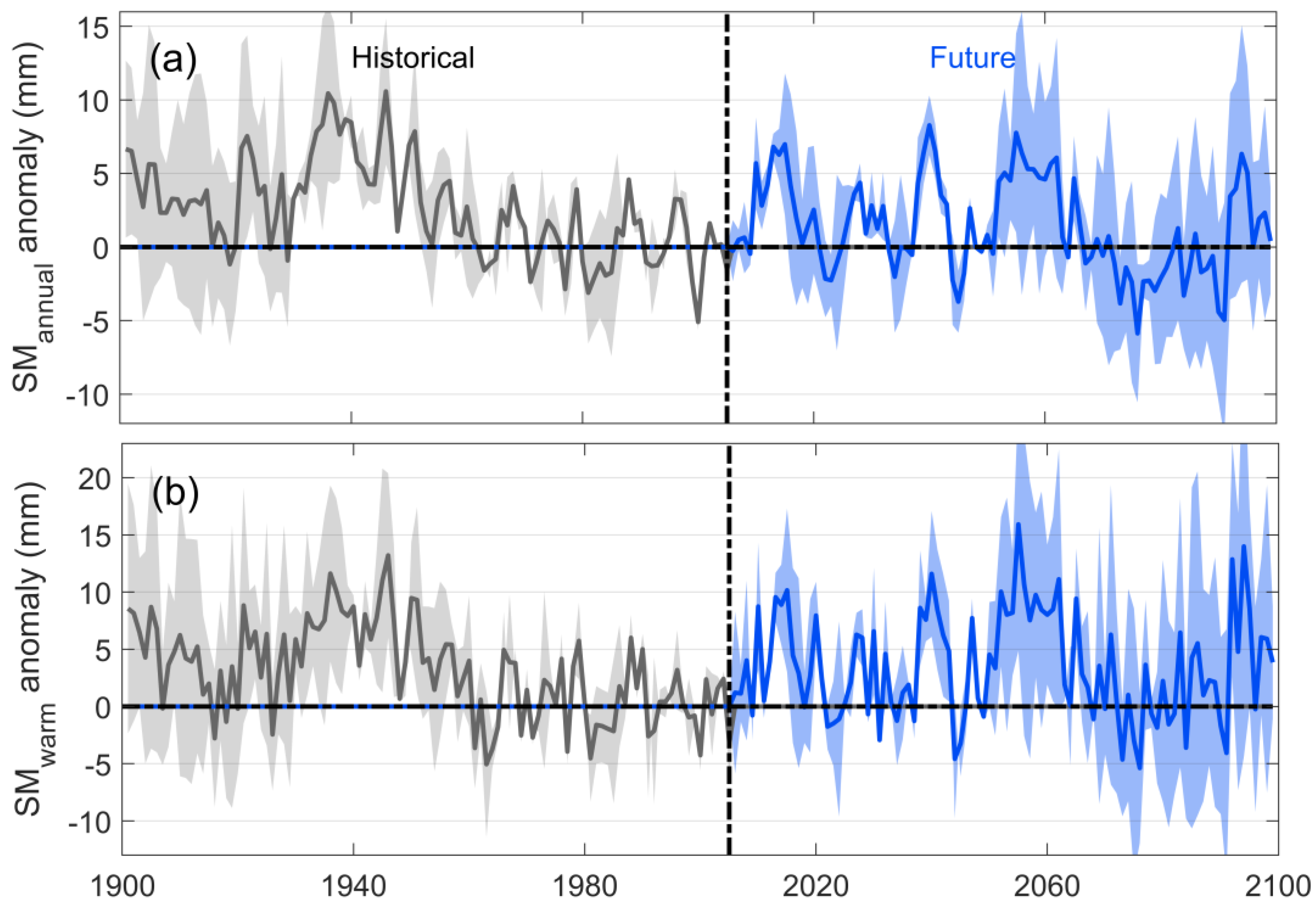
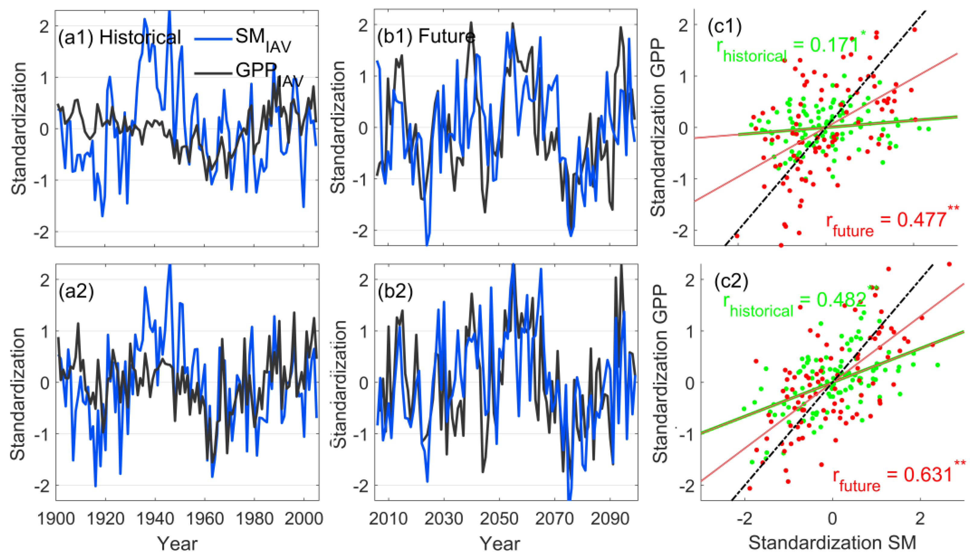
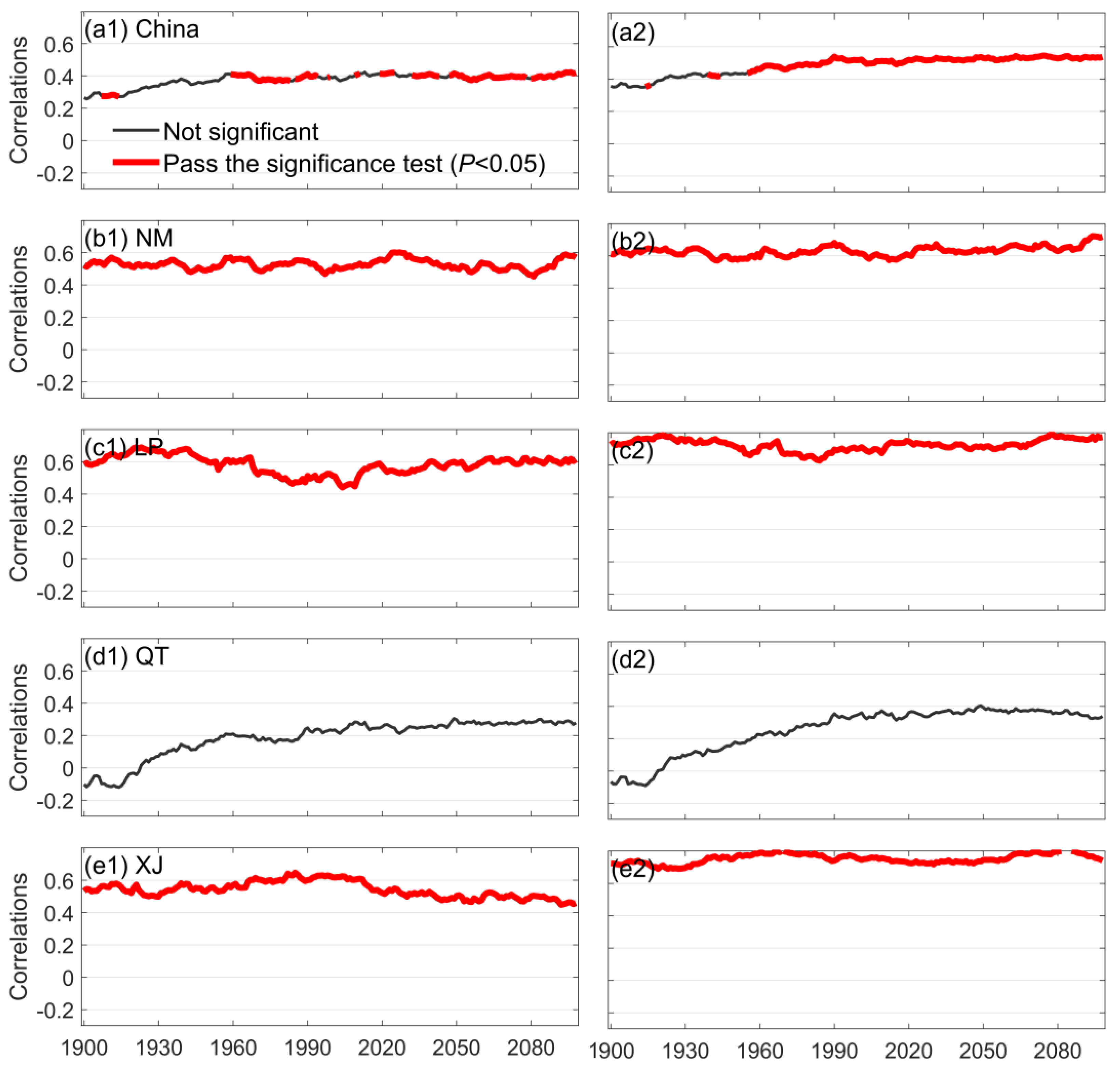
No significant trends were found for soil moisture in the historical or future periods, and its long-term change was mainly reflected through interannual fluctuations. Soil moisture showed a highly significant positive correlation with ecosystem GPP in the time series, indicating that when soil water decreases, it causes a decrease in ecosystem GPP. Moreover, the correlation between SM and GPP was higher in the warm season than annually, and higher in the future period than in the historical period, representing a stronger constraint on GPP in Chinese grasslands in the warm season and a deeper constraint in the future period than in the historical period.
(2)
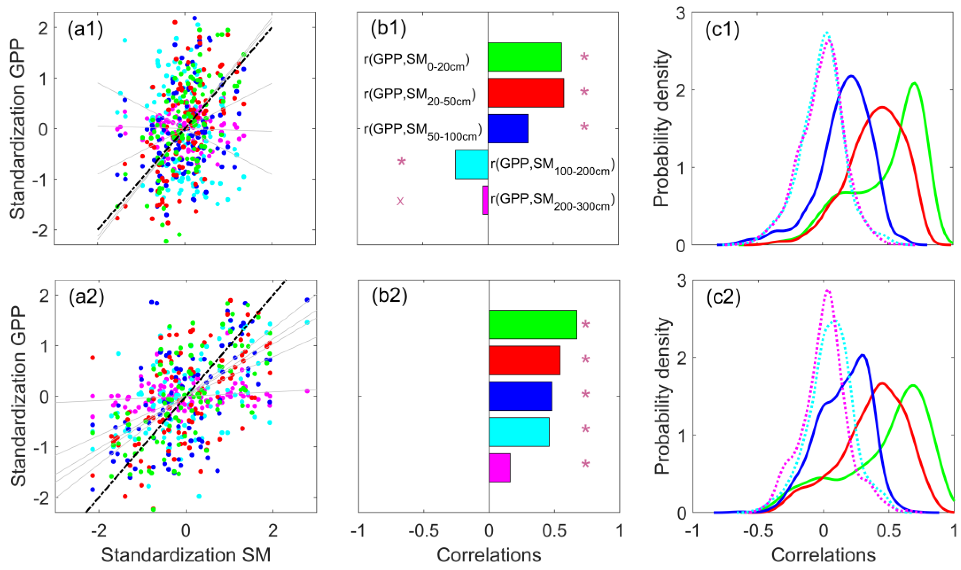
Using the LPJmL model’s soil moisture data at different soil depths and analyzing their relationship with ecosystem GPP, it was found that the correlation between shallow-soil moisture (0–50 cm) and GPP was clearly higher than that of deeper soils, and the probability of an ecosystem GPP deficit due to a shortage of soil water in the shallow layer was much higher than that of soil water in the middle and deep layers.
(3)
In probabilistic terms, soil drought has a higher probability of initiating the loss of ecosystem GPP than atmospheric drought, with moisture scarcity originating from the soil becoming the main aspect that constrains ecosystem GPP. In the future, with the rapid rise of global VPD, the probability of ecosystem GPP loss induced by atmospheric drought increases and overtakes soil drought as the main water constraint in some regions.

Supplementary Materials

The following supporting information can be downloaded at: https://www.mdpi.com/article/10.3390/land12020484/s1, Figure S1.

Author Contributions

Conceptualization, Z.H., Z.S. and P.H.; methodology, X.M. (Xiaoyu Meng) and P.H.; software, T.D., P.H. and N.W.; validation, P.H. and X.M. (Xiaoyu Meng); formal analysis, P.H.; investigation, P.H. and X.M. (Xiaoyu Meng); resources, P.H.; data curation, P.H.; writing—original draft preparation, X.M. (Xiaoliang Ma), Z.H., S.M., and P.H.; writing—review and editing, X.M. (Xiaoliang Ma), X.M. (Xiaoyu Meng), J.M., Y.Z. and P.H.; visualization, P.H.; supervision, P.H.; project administration, Z.S. and P.H.; funding acquisition, Z.S. and P.H. All authors have read and agreed to the published version of the manuscript.

Funding

This research was funded by Foundation items: National Natural Science Foundation of China, No. 32060408; National Basic Resources Survey Special, No. 2017FY100200; the Scientific Innovation Project of Postgraduates of Xinjiang Uygur Autonomous Region, China, No. XJ2021G169.

Institutional Review Board Statement

Not applicable.

Informed Consent Statement

Not applicable.

Data Availability Statement

Data are already published and publicly available, datasets utilized for this research are as follows: The ISIMIP dataset: https://esg.pik-potsdam.de/projects/isimip/, accessed on 6 December 2022.

Conflicts of Interest

The authors declare no conflict of interest.

References

  1. Ciais, P.; Reichstein, M.; Viovy, N.; Granier, A.; Ogee, J.; Allard, V.; Aubinet, M.; Buchmann, N.; Bernhofer, C.; Carrara, A.; et al. Europe-wide reduction in primary productivity caused by the heat and drought in 2003. Nature 2005, 437, 529–533. [Google Scholar] [CrossRef]
  2. Zhao, M.; Running, S. Drought-induced reduction in global terrestrial net primary production from 2000 through 2009. Science 2010, 329, 940–943. [Google Scholar] [CrossRef] [Green Version]
  3. Peng, L.; Xia, J.; Li, Z.; Fang, C.; Deng, X. Spatio-temporal dynamics of water-related disaster risk in the Yangtze River Economic Belt from 2000 to 2015. Resour. Conserv. Recycl. 2020, 161, 104851. [Google Scholar] [CrossRef]
  4. Xiao, J.; Sun, G.; Chen, J.; Chen, H.; Chen, S.; Dong, G.; Gao, S.; Guo, H.; Guo, J.; Han, S.; et al. Carbon fluxes, evapotranspiration, and water use efficiency of terrestrial ecosystems in China. Agric. For. Meteorol. 2013, 182, 76–90. [Google Scholar] [CrossRef]
  5. Yang, Y.; Guan, H.; Batelaan, O.; McVicar, T.; Long, D.; Piao, S.; Liang, W.; Liu, B.; Jin, Z.; Simmons, C. Contrasting response of water use efficiency to drought across global terrestrial ecosystems. Sci. Rep. 2016, 6, 23283. [Google Scholar] [CrossRef] [Green Version]
  6. Zhang, Y.; Xiao, X.; Zhou, S.; Ciais, P.; McCarthy, H.; Luo, Y. Canopy and physiological control of GPP during drought and heatwave. Geophys. Res. Lett. 2016, 43, 3325–3333. [Google Scholar] [CrossRef] [Green Version]
  7. Humphrey, V.; Zscheischler, J.; Ciais, P.; Gudmundsson, L.; Sitch, S.; Seneviratne, S.I. Sensitivity of atmospheric CO2 growth rate to observed changes in terrestrial water storage. Nature 2018, 560, 628–631. [Google Scholar] [CrossRef]
  8. Zhang, J.; Wang, X.; Ren, J. Simulation of Gross Primary Productivity Using Multiple Light Use Efficiency Models. Land 2021, 10, 329. [Google Scholar] [CrossRef]
  9. Liancourt, P.; Sharkhuu, A.; Ariuntsetseg, L.; Boldgiv, B.; Helliker, B.R.; Plante, A.F.; Petraitis, P.S.; Casper, B.B. Temporal and spatial variation in how vegetation alters the soil moisture response to climate manipulation. Plant and Soil 2011, 351, 249–261. [Google Scholar] [CrossRef]
  10. Han, Z.; Huang, Q.; Huang, S.; Leng, G.; Bai, Q.; Liang, H.; Wang, L.; Zhao, J.; Fang, W. Spatial-temporal dynamics of agricultural drought in the Loess Plateau under a changing environment: Characteristics and potential influencing factors. Agric. Water Manag. 2021, 244, 106540. [Google Scholar] [CrossRef]
  11. He, P.; Sun, Z.; Han, Z.; Ma, X.; Zhao, P.; Liu, Y.F.; Ma, J. Divergent trends of water storage observed via gravity satellite across distinct areas in China. Water 2020, 12, 2862. [Google Scholar] [CrossRef]
  12. Sehgal, V.; Gaur, N.; Mohanty, B. Global surface soil moisture drydown patterns. Water Resour. Res. 2021, 57, e2020WR027588. [Google Scholar] [CrossRef]
  13. Yuan, W.; Zheng, Y.; Piao, S.; Ciais, P.; Lombardozzi, D.; Wang, Y.; Ryu, Y.; Chen, G.; Dong, W.; Hu, Z.; et al. Increased atmospheric vapor pressure deficit reduces global vegetation growth. Sci. Adv. 2019, 5, eaax1396. [Google Scholar] [CrossRef] [Green Version]
  14. Shen, Q.; Gao, G.; Fu, B.; Lu, Y. Responses of shelterbelt stand transpiration to drought and groundwater variations in an arid inland river basin of Northwest China. J. Hydrol. 2015, 531, 738–748. [Google Scholar] [CrossRef]
  15. Novick, K.; Ficklin, D.; Stoy, P.; Williams, C.A.; Bohrer, G.; Oishi, A.C.; Papuga, S.A.; Blanken, P.D.; Noormets, A.; Sulman, B.N.; et al. The increasing importance of atmospheric demand for ecosystem water and carbon fluxes. Nat. Clim. Change 2016, 6, 1023–1027. [Google Scholar] [CrossRef] [Green Version]
  16. Liu, L.; Gudmundsson, L.; Hauser, M.; Qin, D.; Li, S.; Seneviratne, S.I. Soil moisture dominates dryness stress on ecosystem production globally. Nat. Commun. 2020, 11, 4892. [Google Scholar] [CrossRef]
  17. Kang, L.; Han, X.; Zhang, Z.; Sun, O.J. Grassland ecosystems in China: Review of current knowledge and research advancement. Philos. Trans. R. Soc. London. Ser. B Biol. Sci. 2007, 362, 997–1008. [Google Scholar] [CrossRef]
  18. Jia, W.; Liu, M.; Wang, D.; He, H.; Shi, P.; Li, Y.; Wang, Y. Uncertainty in simulating regional gross primary productivity from satellite-based models over northern China grassland. Ecol. Indic. 2018, 88, 134–143. [Google Scholar] [CrossRef]
  19. Liu, Y.; Lei, H. Responses of natural vegetation dynamics to climate drivers in China from 1982 to 2011. Remote Sens. 2015, 7, 10243–10268. [Google Scholar] [CrossRef] [Green Version]
  20. Rui, Z.; Zhao, X.; Zuo, X.; Degen, A.; Yulin, L.; Liu, X.; Luo, Y.; Qu, H.; Lian, J.; Wang, R. Drought-induced shift from a carbon sink to a carbon source in the grasslands of Inner Mongolia, China. Catena 2020, 195, 104845. [Google Scholar] [CrossRef]
  21. He, P.; Ma, X.; Sun, Z. Interannual variability in summer climate change controls GPP long-term changes. Environ. Res. 2022, 212, 113409. [Google Scholar] [CrossRef]
  22. Cheng, S.; Huang, J.; Ji, F.; Lin, L. Uncertainties of soil moisture in historical simulations and future projections: Uncertainties of Soil Moisture. J. Geophys. Res. Atmos. 2017, 122, 2239–2253. [Google Scholar] [CrossRef]
  23. Buck, A. New equations for computing vapor pressure and enhancement Factor. J. Appl. Meteorol. 1981, 20, 1527–1532. [Google Scholar] [CrossRef]
  24. Zscheischler, J.; Seneviratne, S. Dependence of drivers affects risks associated with compound events. Sci. Adv. 2017, 3, e1700263. [Google Scholar] [CrossRef] [Green Version]
  25. Bishara, A.; Hittner, J. Testing the significance of a correlation with nonnormal data: Comparison of pearson, spearman, transformation, and resampling approaches. Psychol. Methods 2012, 17, 399–417. [Google Scholar] [CrossRef] [Green Version]
  26. Wang, L.; Huang, S.; Huang, Q.; Leng, G.; Han, Z.; Zhao, J.; Guo, Y. Vegetation vulnerability and resistance to hydrometeorological stresses in water- and energy-limited watersheds based on a Bayesian framework. Catena 2021, 196, 104879. [Google Scholar] [CrossRef]
  27. Jones, M.; Hardle, W. Applied nonparametric regression. Economica 1992, 58, 538. [Google Scholar] [CrossRef] [Green Version]
  28. Wu, Z.; Dijkstra, P.; Koch, G.; Penuelas, J.; Hungate, B. Responses of terrestrial ecosystems to temperature and precipitation change: A meta-analysis of experimental manipulation. Glob. Change Biol. 2011, 17, 927–942. [Google Scholar] [CrossRef] [Green Version]
  29. Shao, C.; Chen, J.; Chu, H.; Lafortezza, R.; Dong, G.; Abraha, M.; Ochirbat, B.; John, R.; Ouyang, Z.; Zhang, Y.; et al. Grassland productivity and carbon sequestration in Mongolian grasslands: The underlying mechanisms and nomadic implications. Environ. Res. 2017, 159, 124–134. [Google Scholar] [CrossRef]
  30. Arca, V.; Power, S.A.; Delgado-Baquerizo, M.; Pendall, E.; Ochoa-Hueso, R. Seasonal effects of altered precipitation regimes on ecosystem-level CO2 fluxes and their drivers in a grassland from Eastern Australia. Plant Soil 2021, 460, 435–451. [Google Scholar] [CrossRef]
  31. Ren, H.; Xu, Z.; Huang, J.; Lü, X.; Zeng, D.-H.; Yuan, Z.; Han, X.; Fang, Y. Increased precipitation induces a positive plant-soil feedback in a semi-arid grassland. Plant Soil 2014, 389, 211–223. [Google Scholar] [CrossRef]
  32. Suttle, K.; Thomsen, M.; Power, M. Species interactions reverse grassland responses to changing climate. Science 2007, 315, 640–642. [Google Scholar] [CrossRef] [Green Version]
  33. Deng, Y.; Wang, X.; Lu, T.; Du, H.; Ciais, P.; Lin, X. Divergent seasonal responses of carbon fluxes to extreme droughts over China. Agric. For. Meteorol. 2023, 328, 109253. [Google Scholar] [CrossRef]
  34. Ru, J.; Zhou, Y.; Hui, D.; Zheng, M.; Wan, S. Shifts of growing-season precipitation peaks decrease soil respiration in a semiarid grassland. Glob. Change Biol. 2017, 24, 1001–1011. [Google Scholar] [CrossRef]
  35. Huxman, T.; Snyder, K.; Tissue, D.; Leffler, A.J.; Ogle, K.; Pockman, W.; Sandquist, D.; Potts, D.; Schwinning, S. Precipitation pulses and carbon fluxes in semiarid and arid ecosystems. Oecologia 2004, 141, 254–268. [Google Scholar] [CrossRef]
  36. Nielsen, U.; Ball, B. Impacts of altered precipitation regimes on soil communities and biogeochemistry in arid and semi-arid ecosystems. Glob. Change Biol. 2014, 21, 1407–1421. [Google Scholar] [CrossRef]
  37. Parton, W.; Morgan, J.; Smith, D.; Del Grosso, S.; Prihodko, L.; Lecain, D.; Kelly, R.; Lutz, S. Impact of precipitation dynamics on net ecosystem productivity. Glob. Change Biol. 2012, 18, 915–927. [Google Scholar] [CrossRef]
  38. Parker, N.; Patrignani, A. Reconstructing Precipitation Events Using Co-located Soil Moisture Information. J. Hydrometeorol. 2021, 22, 3275–3290. [Google Scholar] [CrossRef]
  39. Grossiord, C.; Buckley, T.N.; Cernusak, L.A.; Novick, K.A.; Poulter, B.; Siegwolf, R.T.W.; Sperry, J.S.; McDowell, N.G. Plant responses to rising vapor pressure deficit. New Phytol. 2020, 226, 1550–1566. [Google Scholar] [CrossRef] [Green Version]
  40. He, P.; Ma, X.; Zongjiu, S.; Han, Z.; Ma, S.; Meng, X. Compound drought constrains gross primary productivity in Chinese grasslands. Environ. Res. Lett. 2022, 17, 104054. [Google Scholar] [CrossRef]
  41. Allen-Diaz, B.H. Water Table and Plant Species Relationships in Sierra Nevada Meadows. Am. Midl. Nat. 1991, 126, 30–43. [Google Scholar] [CrossRef]
  42. Darrouzet-Nardi, A.; D’Antonio, C.M.; Dawson, T.E. Depth of water acquisition by invading shrubs and resident herbs in a Sierra Nevada meadow. Plant Soil 2006, 285, 31–43. [Google Scholar] [CrossRef]
  43. Hoekstra, N.; Finn, J.; Hofer, D.; Luscher, A. The effect of drought and interspecific interactions on depth of water uptake in deep- and shallow-rooting grassland species as determined by delta O-18 natural abundance. Biogeosciences 2014, 11, 4493–4506. [Google Scholar] [CrossRef] [Green Version]
  44. Yongming, C.; Liu, L.; Cheng, L.; Fa, K.; Liu, X.; Huo, Z.; Huang, G. A shift in the dominant role of atmospheric vapor pressure deficit and soil moisture on vegetation greening in China. J. Hydrol. 2023, 615, 128680. [Google Scholar] [CrossRef]
Figure 1. Long-term variation in soil moisture anomalies based on process-model simulations. (a) Annual SM; (b) warm-season SM. SM anomalies are relative to the distance to the mean during 2006–2015. The shaded line is the doubled standard deviation between the four models. The warm seasons mentioned are the three months with the largest annual mean temperatures in 1901–2005.
Land 12 00484 g001
Figure 2. Standardized interannual variability characteristics of soil moisture (SMIAV) and gross primary productivity (GPPIAV) in Chinese grasslands. The upper side shows the annual time series, and the lower side shows the warm-season time series. (a) historical period; (b) future period; (c) correlation between SMIAV and GPPIAV per year, * represents passing 0.1 significance test, and ** represents passing 0.05 significance test.
Land 12 00484 g002
Figure 3. Correlation between GPPIAV and SMIAV for Chinese grasslands during the period 1901–2099. (a1,b1,c1,d1,e1) is annual, and (a2,b2,c2,d2,e2) is the warm season. The correlation between SMIAV and GPPIAV per year in the warm season was calculated with a 41-year sliding window, i.e., by calculating the correlation between the two variables from 1861–1901 as the result in 1901, and so on, to find the correlation from 1901–2099. The red line in the figure shows the years in which the correlations passed the significance test (p < 0.05).
Land 12 00484 g003
Figure 4. Correlation between warm-season SM and GPP for different soil depths. The upper column is the historical period and the lower column is the future period. (a1,a2) Scatter plots of SM and GPP per year. Red, green, blue, cyan, and pink represent soil moisture at 0–20 cm, 20–50 cm, 50–100 mm, 100–200 mm, and 200–300 mm soil depths, respectively; (b1,b2) correlation between SM and GPP regional averages; (c1,c2) probability density plot of correlation between SM and GPP.
Land 12 00484 g004
Figure 5. Conditional probabilities of ecosystem GPP loss under severe soil drought conditions (i.e., probability when soil moisture is below 10% threshold in the 1901–2005 time series) at different soil depths of Chinese grasslands during the historical period. (a1a6,b1b6,c1c6) The probability of severe ecosystem GPP loss under severe soil drought conditions; 1–6 represent the soil depths of 0–300 mm, 0–20 mm, 20–50 mm, 50–100 mm, 100–200 mm, and 200–300 mm, respectively. The regional average trend values are counted as box plots in the lower left corner. NM, LP, QT, and XJ represent grasslands in Inner Mongolia, the Loess Plateau, the Tibetan Plateau, and Xinjiang, respectively, and red dots represent anomalies. The histogram is the frequency statistics.
Land 12 00484 g005
Figure 6. Difference between the probability of ecosystem GPP loss under soil drought conditions minus the probability of ecosystem GPP loss in the atmospheric drought scenario for the historical period. (ac) The difference between the probability of severe, moderate, and mild ecosystem GPP loss corresponding to severe soil drought and atmospheric drought; (df) the difference between the probability of severe, moderate, and mild ecosystem GPP loss corresponding to moderate soil drought and atmospheric drought; (gi) the difference between the probability of severe, moderate, and mild ecosystem GPP loss corresponding to mild soil drought and atmospheric drought; (gi) the difference in the probability of severe, moderate, and mild ecosystem GPP loss corresponding to mild soil and atmospheric drought.
Land 12 00484 g006
Figure 7. Difference between the probability of ecosystem GPP loss under soil drought conditions minus the probability of ecosystem GPP loss in the atmospheric drought scenario for the future period. (ac) The difference between the probability of severe, moderate, and mild ecosystem GPP loss corresponding to severe soil drought and atmospheric drought; (df) the difference between the probability of severe, moderate, and mild ecosystem GPP loss corresponding to moderate soil drought and atmospheric drought; (gi) the difference between the probability of severe, moderate, and mild ecosystem GPP loss corresponding to mild soil drought and atmospheric drought; (gi) the difference in the probability of severe, moderate, and mild ecosystem GPP loss corresponding to mild soil and atmospheric drought..
Land 12 00484 g007
Table 1. Expressions of marginal distribution function.
CopulaExpression of Distribution Function C(u,v)Range of θ Values
Clayton m a x u - θ + v - θ - 1 - 1 / θ , 0 0 , +
Frank - 1 θ l n 1 + e - θ u - 1 e - θ v - 1 e - θ - 1 - , 0 0 , +
Gumbel e x p - - ln u θ + - ln v θ 1 / θ 1 , +
t - t k - 1 u - t k - 1 v 1 2 π 1 - θ 2 e x p 1 + s 2 - 2 θ s t + t 2 k 1 - θ 2 - k + 2 2 d s d t - 1,1 , k 0
Gaussian - - 1 u - - 1 v 1 2 π 1 - θ 2 e x p 1 + s 2 - 2 θ s t + t 2 k 1 - θ 2 - k + 2 2 d s d t - 1,1 , k 0
Disclaimer/Publisher’s Note: The statements, opinions and data contained in all publications are solely those of the individual author(s) and contributor(s) and not of MDPI and/or the editor(s). MDPI and/or the editor(s) disclaim responsibility for any injury to people or property resulting from any ideas, methods, instructions or products referred to in the content.

