
Synergetic Integration of SWAT and Multi-Objective Optimization Algorithms for Evaluating Efficiencies of Agricultural Best Management Practices to Improve Water Quality


Abstract
:1. Introduction
- Develop a hydrological model for the simulation of streamflow and nitrate loading;
- Evaluate the effects of different combinations of BMPs on nitrogen load reduction;
- Explore the optimal combinations of BMPs and the best set of decisions that can control the water quality of the Jajrood river.
2. Materials and Methods
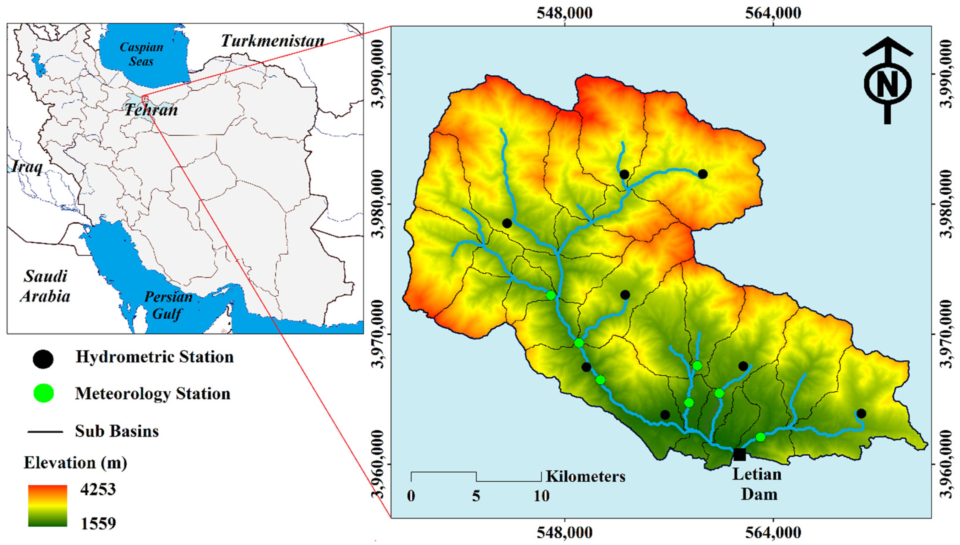
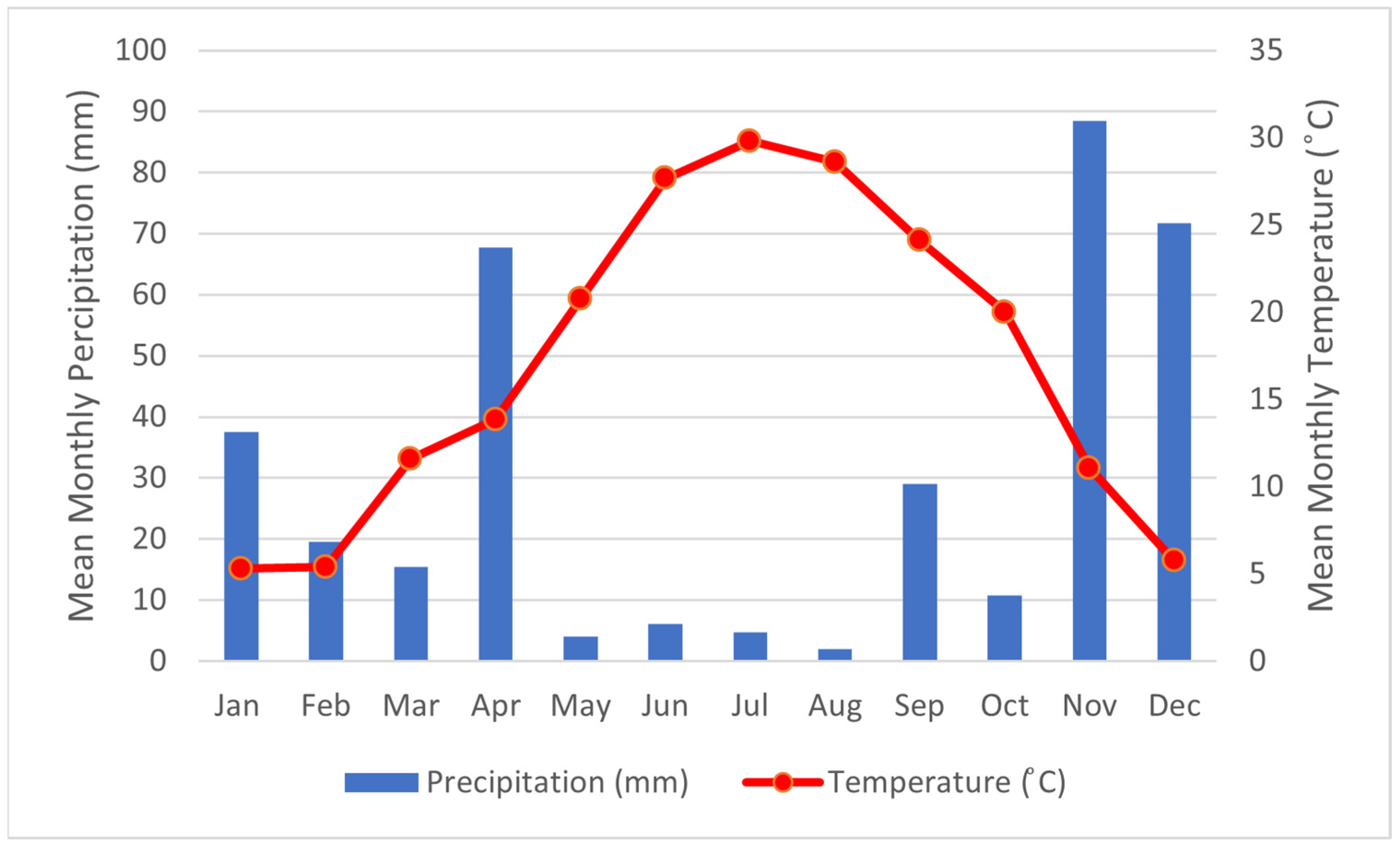
2.1. Study Area
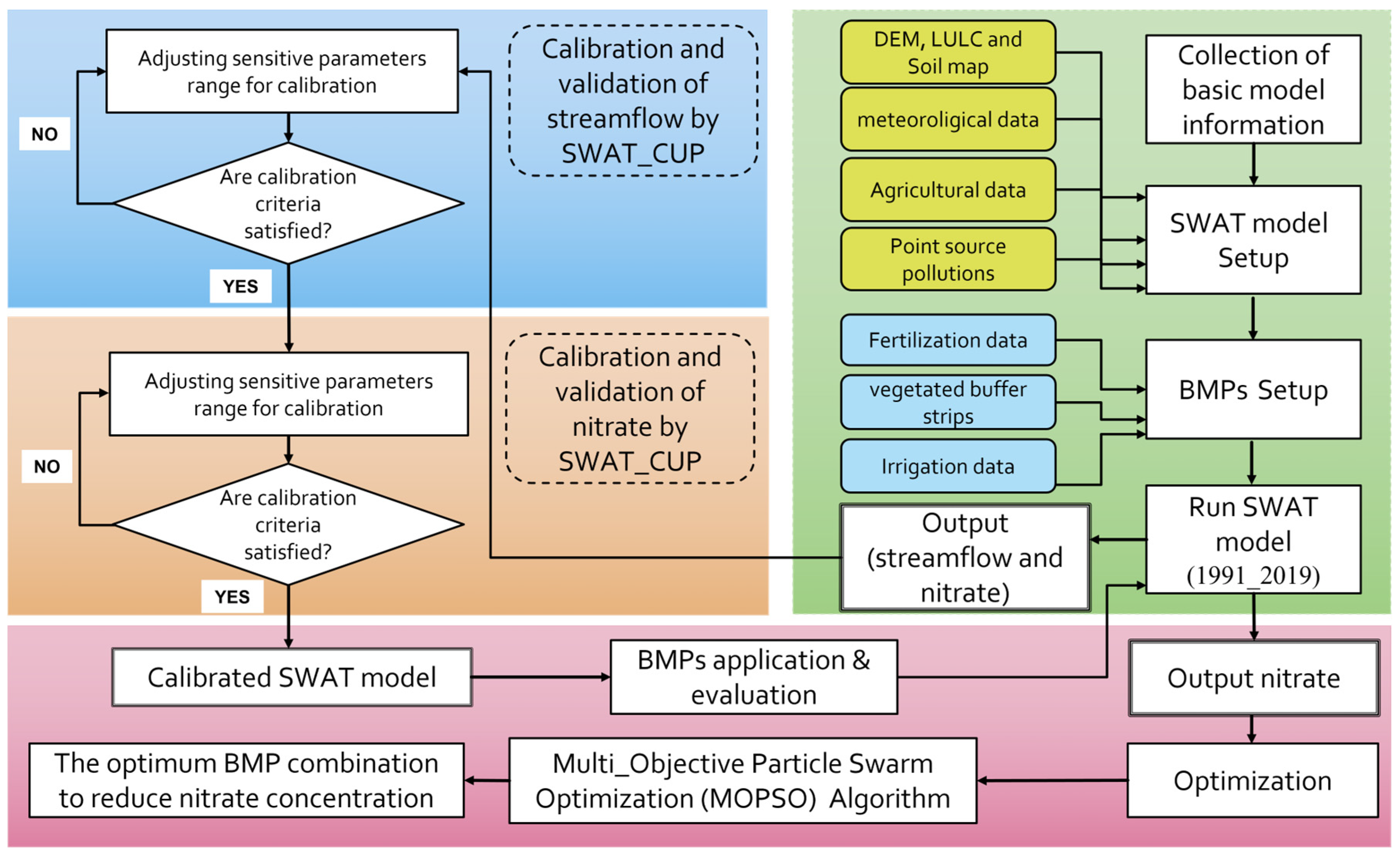
2.2. Research Methodology
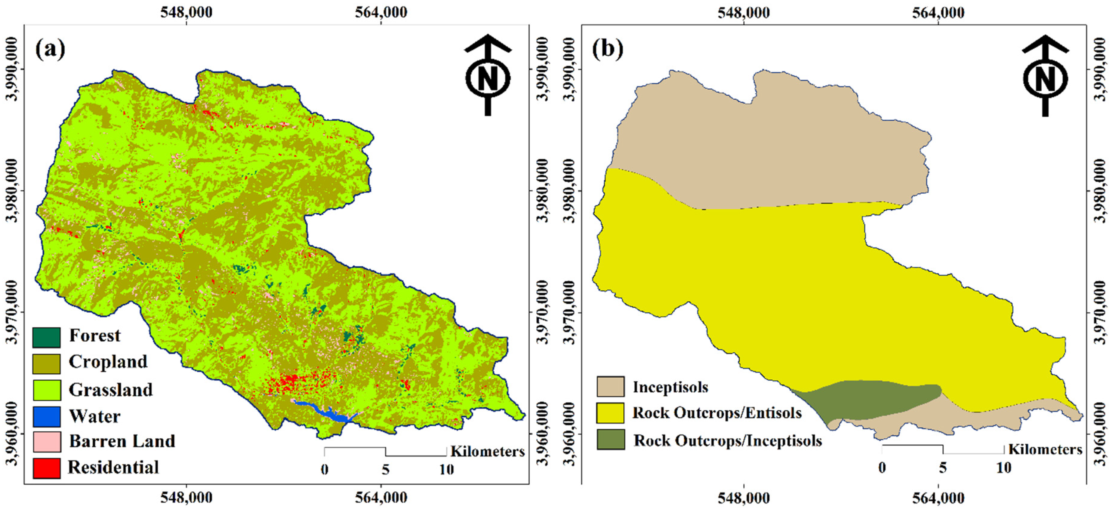
2.3. SWAT Model and Input Dataset
Sensitivity Analysis of Model Parameters, Calibration, and Validation
2.4. Evaluating the Performance of BMPs
2.4.1. Fertilizer Management
2.4.2. Vegetated Filter Strips
2.4.3. Irrigation Management
2.5. Qualitative Optimization of the Model
3. Results
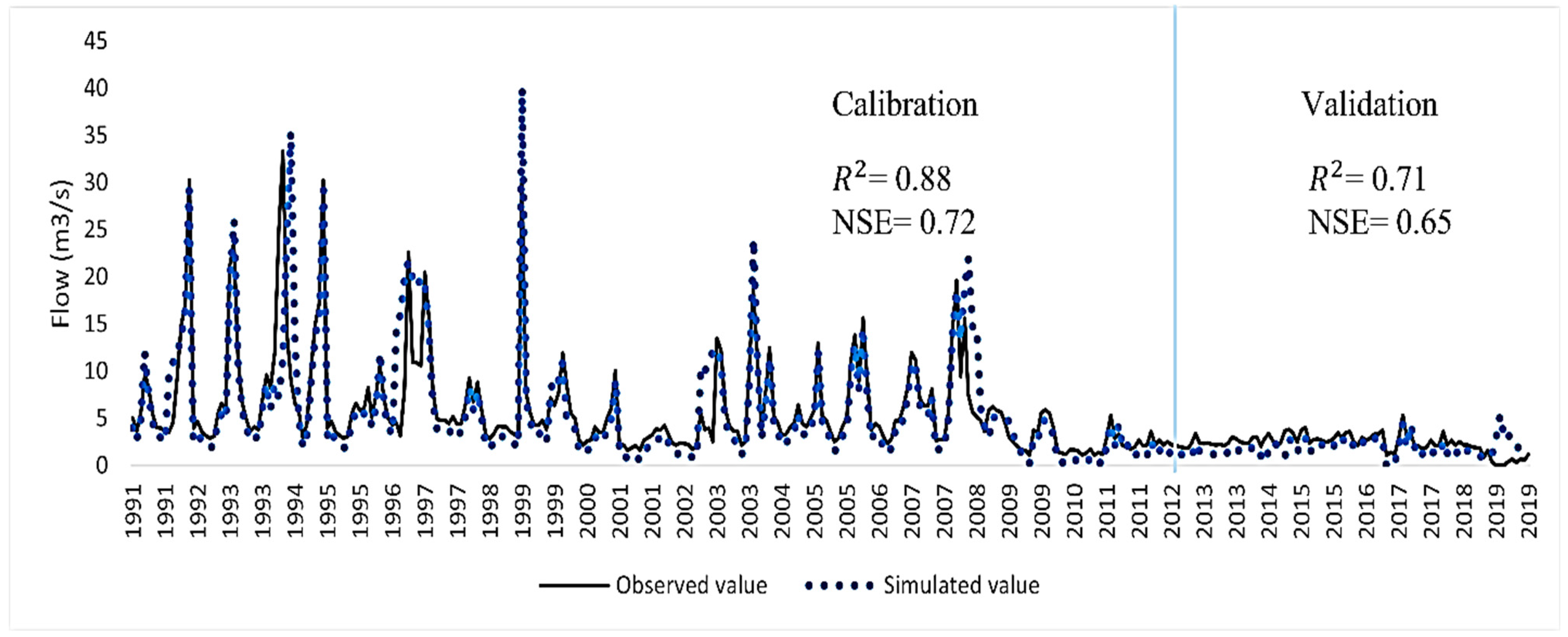
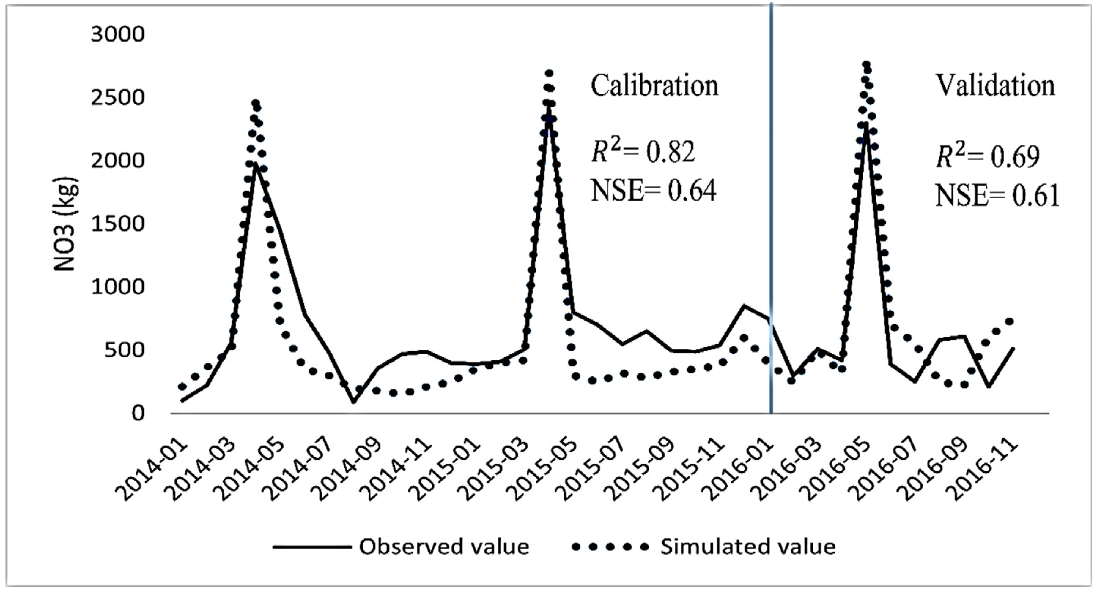
3.1. Calibration and Validation Results for Streamflow and Nitrate
3.2. Investigating the Effect of BMPs on the Water Quality
3.2.1. Fertilizer Management
3.2.2. Vegetated Filter Strips
3.2.3. Irrigation Management
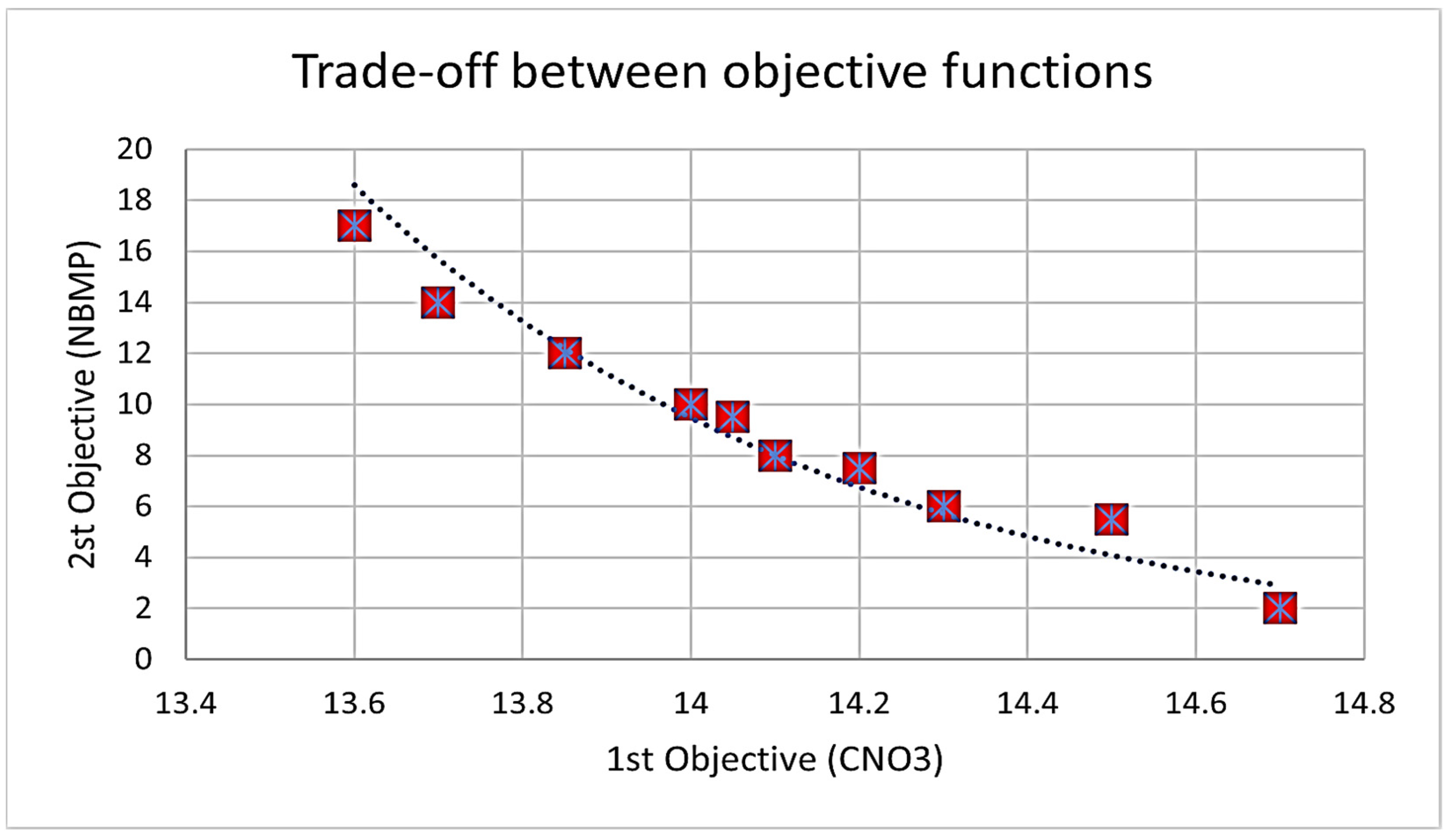
3.3. Results of Qualitative Optimization of the Model with the MOPSO Algorithm
4. Discussion
5. Conclusions
Author Contributions
Funding
Data Availability Statement
Conflicts of Interest
Appendix A

| Parameter | Description |
|---|---|
| TLAPS | The temperature lapse rate |
| GW_DELAY | Groundwater delay time |
| SNOCOVMX | The fraction of snow volume |
| CN2 | The initial SCS runoff curve number for moisture condition |
| ALPHA_BF | The baseflow alpha factor |
| SFTMP | The snowfall temperature |
| ESCO | The compensation coefficient |
| TIMP | The snow temperature lag factor |
| SURLAG | The surface runoff lag coefficient |
| SLSUBBSN | The average slope length |
| Parameter | Description |
|---|---|
| ERORGN | The organic nitrogen enrichment ratio |
| NPERCO | Nitrogen percolation coefficient |
| RCN | The nitrogen concentration in rainfall |
| BC3_BSN | The rate constant for the hydrolysis of organic nitrogen to ammonia |
| BC2_BSN | Rate constant for biological oxidation of NO2 to NO3 |
| FO 1 | RE 2 | CR 3 | GR 4 | WA 5 | BL 6 | |
|---|---|---|---|---|---|---|
| FO | 1000 | 0 | 2 | 1 | 0 | 0 |
| RE | 0 | 200 | 0 | 16 | 0 | 12 |
| CR | 10 | 4 | 3077 | 132 | 18 | 20 |
| GR | 0 | 0 | 130 | 2208 | 18 | 29 |
| WA | 2 | 0 | 5 | 12 | 528 | 5 |
| BL | 0 | 0 | 12 | 30 | 31 | 242 |
| UA 7 | 98.81 | 98.04 | 95.38 | 92.04 | 88.74 | 78.57 |
| PA 8 | 99.70 | 87.72 | 94.36 | 92.58 | 95.65 | 76.83 |
| Kappa | 91.06% | |||||
| OA 9 | 93.11% | |||||
References
- Tickner, D.; Parker, H.; Moncrieff, C.R.; Oates, N.E.; Ludi, E.; Acreman, M. Managing rivers for multiple benefits—A coherent approach to research, policy and planning. Front. Environ. Sci. 2017, 5, 4. [Google Scholar] [CrossRef]
- Jia, G.; Hu, W.; Zhang, B.; Li, G.; Shen, S.; Gao, Z.; Li, Y. Assessing impacts of the Ecological Retreat project on water conservation in the Yellow River Basin. Sci. Total Environ. 2022, 828, 154483. [Google Scholar] [CrossRef]
- Sattar, M.A.; Kroeze, C.; Strokal, M. The increasing impact of food production on nutrient export by rivers to the Bay of Bengal 1970–2050. Mar. Pollut. Bull. 2014, 80, 168–178. [Google Scholar] [CrossRef] [PubMed]
- Jägermeyr, J.; Pastor, A.; Biemans, H.; Gerten, D. Reconciling irrigated food production with environmental flows for Sustainable Development Goals implementation. Nat. Commun. 2017, 8, 15900. [Google Scholar] [CrossRef] [PubMed]
- Wohl, E.; Dwire, K.; Sutfin, N.; Polvi, L.; Bazan, R. Mechanisms of carbon storage in mountainous headwater rivers. Nat. Commun. 2012, 3, 1263. [Google Scholar] [CrossRef]
- Sutfin, N.A.; Wohl, E.E.; Dwire, K.A. Banking carbon: A review of organic carbon storage and physical factors influencing retention in floodplains and riparian ecosystems. Earth Surf. Process. Landf. 2016, 41, 38–60. [Google Scholar] [CrossRef]
- Ward, P.J.; Jongman, B.; Aerts, J.C.; Bates, P.D.; Botzen, W.J.; Diaz Loaiza, A.; Hallegatte, S.; Kind, J.M.; Kwadijk, J.; Scussolini, P. A global framework for future costs and benefits of river-flood protection in urban areas. Nat. Clim. Change 2017, 7, 642–646. [Google Scholar] [CrossRef]
- Santoro, S.; Pluchinotta, I.; Pagano, A.; Pengal, P.; Cokan, B.; Giordano, R. Assessing stakeholders’ risk perception to promote Nature Based Solutions as flood protection strategies: The case of the Glinščica river (Slovenia). Sci. Total Environ. 2019, 655, 188–201. [Google Scholar] [CrossRef] [PubMed]
- Björklund, K.; Bondelind, M.; Karlsson, A.; Karlsson, D.; Sokolova, E. Hydrodynamic modelling of the influence of stormwater and combined sewer overflows on receiving water quality: Benzo (a) pyrene and copper risks to recreational water. J. Environ. Manag. 2018, 207, 32–42. [Google Scholar] [CrossRef]
- Xin, Z.; Ye, L.; Zhang, C. Application of export coefficient model and QUAL2K for water environmental management in a Rural Watershed. Sustainability 2019, 11, 6022. [Google Scholar] [CrossRef] [Green Version]
- Akhtar, N.; Syakir Ishak, M.I.; Bhawani, S.A.; Umar, K. Various natural and anthropogenic factors responsible for water quality degradation: A review. Water 2021, 13, 2660. [Google Scholar] [CrossRef]
- Belhassan, K.; Vaseashta, A.; Hessane, M.A.; Kaabar, M.K.; Hussein, E.K.; Adnan, M.; Rasouli, H. Potential impact of drought on Mikkes river flow (Morocco). Iran. J. Earth Sci. 2022. [Google Scholar] [CrossRef]
- Berbel, J.; Esteban, E. Droughts as a catalyst for water policy change. Analysis of Spain, Australia (MDB), and California. Glob. Environ. Change 2019, 58, 101969. [Google Scholar] [CrossRef]
- Henao Casas, J.; Fernández Escalante, E.; Ayuga, F. Alleviating drought and water scarcity in the Mediterranean region through managed aquifer recharge. Hydrogeol. J. 2022, 30, 1685–1699. [Google Scholar] [CrossRef]
- Didovets, I.; Krysanova, V.; Bürger, G.; Snizhko, S.; Balabukh, V.; Bronstert, A. Climate change impact on regional floods in the Carpathian region. J. Hydrol. Reg. Stud. 2019, 22, 100590. [Google Scholar] [CrossRef]
- Pal, S.C.; Chowdhuri, I.; Das, B.; Chakrabortty, R.; Roy, P.; Saha, A.; Shit, M. Threats of climate change and land use patterns enhance the susceptibility of future floods in India. J. Environ. Manag. 2022, 305, 114317. [Google Scholar] [CrossRef]
- Rai, R.K.; Shyamsundar, P.; Nepal, M.; Bhatta, L.D. Financing watershed services in the foothills of the Himalayas. Water 2018, 10, 965. [Google Scholar] [CrossRef]
- Pham, N.T.T.; Nong, D.; Sathyan, A.R.; Garschagen, M. Vulnerability assessment of households to flash floods and landslides in the poor upland regions of Vietnam. Clim. Risk Manag. 2020, 28, 100215. [Google Scholar] [CrossRef]
- Azimi Sardari, M.R.; Bazrafshan, O.; Panagopoulos, T.; Sardooi, E.R. Modeling the impact of climate change and land use change scenarios on soil erosion at the Minab Dam Watershed. Sustainability 2019, 11, 3353. [Google Scholar] [CrossRef]
- Kumarasiri, A.; Udayakumara, E.; Jayawardana, J. Impacts of soil erosion and forest quality on water quality in Samanalawewa watershed, Sri Lanka. Model. Earth Syst. Environ. 2022, 8, 529–544. [Google Scholar] [CrossRef]
- Abedin, M.; Collins, A.E.; Habiba, U.; Shaw, R. Climate change, water scarcity, and health adaptation in southwestern coastal Bangladesh. Int. J. Disaster Risk Sci. 2019, 10, 28–42. [Google Scholar] [CrossRef]
- Zobeidi, T.; Yaghoubi, J.; Yazdanpanah, M. Farmers’ incremental adaptation to water scarcity: An application of the model of private proactive adaptation to climate change (MPPACC). Agric. Water Manag. 2022, 264, 107528. [Google Scholar] [CrossRef]
- Baccour, S.; Albiac, J.; Kahil, T.; Esteban, E.; Crespo, D.; Dinar, A. Hydroeconomic modeling for assessing water scarcity and agricultural pollution abatement policies in the Ebro River Basin, Spain. J. Clean. Prod. 2021, 327, 129459. [Google Scholar] [CrossRef]
- Vaseashta, A.; Gevorgyan, G.; Kavaz, D.; Ivanov, O.; Jawaid, M.; Vasović, D. Exposome, biomonitoring, assessment and data analytics to quantify universal water quality. In Water Safety, Security and Sustainability; Springer: Berlin/Heidelberg, Germany, 2021; pp. 67–114. [Google Scholar]
- Xiang, X.; Li, Q.; Khan, S.; Khalaf, O.I. Urban water resource management for sustainable environment planning using artificial intelligence techniques. Environ. Impact Assess. Rev. 2021, 86, 106515. [Google Scholar] [CrossRef]
- Merriman, K.R.; Russell, A.M.; Rachol, C.M.; Daggupati, P.; Srinivasan, R.; Hayhurst, B.A.; Stuntebeck, T.D. Calibration of a field-scale soil and water assessment tool (SWAT) model with field placement of best management practices in Alger Creek, Michigan. Sustainability 2018, 10, 851. [Google Scholar] [CrossRef]
- Wang, J.; Guo, Y. Dynamic water balance of infiltration-based stormwater best management practices. J. Hydrol. 2020, 589, 125174. [Google Scholar] [CrossRef]
- Song, J.; Yang, Y.; Sun, X.; Lin, J.; Wu, M.; Wu, J.; Wu, J. Basin-scale multi-objective simulation-optimization modeling for conjunctive use of surface water and groundwater in northwest China. Hydrol. Earth Syst. Sci. 2020, 24, 2323–2341. [Google Scholar] [CrossRef]
- Taheriyoun, M.; Fallahi, A.; Nazari-Sharabian, M.; Fallahi, S. Optimization of best management practices to control runoff water quality in an urban watershed using a novel framework of embedding-response surface model. J. Hydro-Environ. Res. 2023, 46, 19–30. [Google Scholar] [CrossRef]
- Kieta, K.A.; Owens, P.N.; Vanrobaeys, J.A.; Lobb, D.A. Seasonal changes in phosphorus in soils and vegetation of vegetated filter strips in cold climate agricultural systems. Agriculture 2022, 12, 233. [Google Scholar] [CrossRef]
- Yu, C.; Duan, P.; Yu, Z.; Gao, B. Experimental and model investigations of vegetative filter strips for contaminant removal: A review. Ecol. Eng. 2019, 126, 25–36. [Google Scholar] [CrossRef]
- Gathagu, J.N.; Mourad, K.A.; Sang, J. Effectiveness of contour farming and filter strips on ecosystem services. Water 2018, 10, 1312. [Google Scholar] [CrossRef]
- Noreika, N.; Li, T.; Winterova, J.; Krasa, J.; Dostal, T. The effects of agricultural conservation practices on the small water cycle: From the farm-to the management-scale. Land 2022, 11, 683. [Google Scholar] [CrossRef]
- Bargaz, A.; Lyamlouli, K.; Chtouki, M.; Zeroual, Y.; Dhiba, D. Soil microbial resources for improving fertilizers efficiency in an integrated plant nutrient management system. Front. Microbiol. 2018, 9, 1606. [Google Scholar] [CrossRef]
- Yadav, G.S.; Lal, R.; Meena, R.S.; Babu, S.; Das, A.; Bhowmik, S.; Datta, M.; Layak, J.; Saha, P. Conservation tillage and nutrient management effects on productivity and soil carbon sequestration under double cropping of rice in north eastern region of India. Ecol. Indic. 2019, 105, 303–315. [Google Scholar] [CrossRef]
- Crystal-Ornelas, R.; Thapa, R.; Tully, K.L. Soil organic carbon is affected by organic amendments, conservation tillage, and cover cropping in organic farming systems: A meta-analysis. Agric. Ecosyst. Environ. 2021, 312, 107356. [Google Scholar] [CrossRef]
- Lozier, T.; Macrae, M.; Brunke, R.; Van Eerd, L. Release of phosphorus from crop residue and cover crops over the non-growing season in a cool temperate region. Agric. Water Manag. 2017, 189, 39–51. [Google Scholar] [CrossRef]
- Schilling, K.E.; Kult, K.; Wilke, K.; Streeter, M.; Vogelgesang, J. Nitrate reduction in a reconstructed floodplain oxbow fed by tile drainage. Ecol. Eng. 2017, 102, 98–107. [Google Scholar] [CrossRef]
- Li, P.; Muenich, R.L.; Chaubey, I.; Wei, X. Evaluating agricultural BMP effectiveness in improving freshwater provisioning under changing climate. Water Resour. Manag. 2019, 33, 453–473. [Google Scholar] [CrossRef]
- Ricci, G.F.; D’Ambrosio, E.; De Girolamo, A.M.; Gentile, F. Efficiency and feasibility of best management practices to reduce nutrient loads in an agricultural river basin. Agric. Water Manag. 2022, 259, 107241. [Google Scholar] [CrossRef]
- Rohmat, F.I.; Gates, T.K.; Labadie, J.W. Enabling improved water and environmental management in an irrigated river basin using multi-agent optimization of reservoir operations. Environ. Model. Softw. 2021, 135, 104909. [Google Scholar] [CrossRef]
- Wei, X.; Bailey, R.T. Evaluating nitrate and phosphorus remediation in intensively irrigated stream-aquifer systems using a coupled flow and reactive transport model. J. Hydrol. 2021, 598, 126304. [Google Scholar] [CrossRef]
- Liu, Y.; Guo, T.; Wang, R.; Engel, B.A.; Flanagan, D.C.; Li, S.; Pijanowski, B.C.; Collingsworth, P.D.; Lee, J.G.; Wallace, C.W. A SWAT-based optimization tool for obtaining cost-effective strategies for agricultural conservation practice implementation at watershed scales. Sci. Total Environ. 2019, 691, 685–696. [Google Scholar] [CrossRef] [PubMed]
- Palmate, S.S.; Pandey, A. Effectiveness of best management practices on dependable flows in a river basin using hydrological SWAT model. In Water Management and Water Governance; Springer: Berlin/Heidelberg, Germany, 2021; pp. 335–348. [Google Scholar]
- Dong, F.; Liu, Y.; Wu, Z.; Chen, Y.; Guo, H. Identification of watershed priority management areas under water quality constraints: A simulation-optimization approach with ideal load reduction. J. Hydrol. 2018, 562, 577–588. [Google Scholar] [CrossRef]
- Emami Skardi, M.J.; Afshar, A.; Saadatpour, M.; Sandoval Solis, S. Hybrid ACO–ANN-based multi-objective simulation–optimization model for pollutant load control at basin scale. Environ. Model. Assess. 2015, 20, 29–39. [Google Scholar] [CrossRef]
- Dong, F.; Li, J.; Dai, C.; Niu, J.; Chen, Y.; Huang, J.; Liu, Y. Understanding robustness in multiscale nutrient abatement: Probabilistic simulation-optimization using Bayesian network emulators. J. Clean. Prod. 2022, 378, 134394. [Google Scholar] [CrossRef]
- Yu, X.; Sreekanth, J.; Cui, T.; Pickett, T.; Xin, P. Adaptative DNN emulator-enabled multi-objective optimization to manage aquifer− sea flux interactions in a regional coastal aquifer. Agric. Water Manag. 2021, 245, 106571. [Google Scholar] [CrossRef]
- Zhang, X.; Srinivasan, R.; Zhao, K.; Liew, M.V. Evaluation of global optimization algorithms for parameter calibration of a computationally intensive hydrologic model. Hydrol. Process. Int. J. 2009, 23, 430–441. [Google Scholar] [CrossRef]
- Aalami, M.T.; Abbasi, H.; Nourani, V. Sustainable management of reservoir water quality and quantity through reservoir operational strategy and watershed control strategies. Int. J. Environ. Res. 2018, 12, 773–788. [Google Scholar] [CrossRef]
- Taghizadeh, S.; Khani, S.; Rajaee, T. Hybrid SWMM and particle swarm optimization model for urban runoff water quality control by using green infrastructures (LID-BMPs). Urban For. Urban Green. 2021, 60, 127032. [Google Scholar] [CrossRef]
- López-Ballesteros, A.; Senent-Aparicio, J.; Srinivasan, R.; Pérez-Sánchez, J. Assessing the impact of best management practices in a highly anthropogenic and ungauged watershed using the SWAT model: A case study in the El Beal Watershed (Southeast Spain). Agronomy 2019, 9, 576. [Google Scholar] [CrossRef] [Green Version]
- Himanshu, S.K.; Pandey, A.; Yadav, B.; Gupta, A. Evaluation of best management practices for sediment and nutrient loss control using SWAT model. Soil Tillage Res. 2019, 192, 42–58. [Google Scholar] [CrossRef]
- Liu, G.; Chen, L.; Wang, W.; Sun, C.; Shen, Z. A water quality management methodology for optimizing best management practices considering changes in long-term efficiency. Sci. Total Environ. 2020, 725, 138091. [Google Scholar] [CrossRef] [PubMed]
- Abdelmalik, K. Role of statistical remote sensing for Inland water quality parameters prediction. Egypt. J. Remote Sens. Space Sci. 2018, 21, 193–200. [Google Scholar] [CrossRef]
- Sagan, V.; Peterson, K.T.; Maimaitijiang, M.; Sidike, P.; Sloan, J.; Greeling, B.A.; Maalouf, S.; Adams, C. Monitoring inland water quality using remote sensing: Potential and limitations of spectral indices, bio-optical simulations, machine learning, and cloud computing. Earth-Sci. Rev. 2020, 205, 103187. [Google Scholar] [CrossRef]
- Topp, S.N.; Pavelsky, T.M.; Jensen, D.; Simard, M.; Ross, M.R. Research trends in the use of remote sensing for inland water quality science: Moving towards multidisciplinary applications. Water 2020, 12, 169. [Google Scholar] [CrossRef]
- Li, T.; Jeřábek, J.; Noreika, N.; Dostál, T.; Zumr, D. An overview of hydrometeorological datasets from a small agricultural catchment (Nučice) in the Czech Republic. Hydrol. Process. 2021, 35, e14042. [Google Scholar] [CrossRef]
- Puczko, K.; Jekatierynczuk-Rudczyk, E. Extreme hydro-meteorological events influence to water quality of small rivers in urban area: A case study in Northeast Poland. Sci. Rep. 2020, 10, 10255. [Google Scholar] [CrossRef]
- Gibson, K.E.; Gibson, J.P.; Grassini, P. Benchmarking irrigation water use in producer fields in the US central Great Plains. Environ. Res. Lett. 2019, 14, 054009. [Google Scholar] [CrossRef]
- Yang, L.; Shen, F.; Zhang, L.; Cai, Y.; Yi, F.; Zhou, C. Quantifying influences of natural and anthropogenic factors on vegetation changes using structural equation modeling: A case study in Jiangsu Province, China. J. Clean. Prod. 2021, 280, 124330. [Google Scholar] [CrossRef]
- Hashemi Aslani, Z.; Omidvar, B.; Karbassi, A. Integrated model for land-use transformation analysis based on multi-layer perception neural network and agent-based model. Environ. Sci. Pollut. Res. 2022, 29, 59770–59783. [Google Scholar] [CrossRef]
- Ustaoğlu, F.; Tepe, Y.; Taş, B. Assessment of stream quality and health risk in a subtropical Turkey river system: A combined approach using statistical analysis and water quality index. Ecol. Indic. 2020, 113, 105815. [Google Scholar] [CrossRef]
- Bussi, G.; Whitehead, P.G.; Jin, L.; Taye, M.T.; Dyer, E.; Hirpa, F.A.; Yimer, Y.A.; Charles, K.J. Impacts of climate change and population growth on river nutrient loads in a data scarce region: The Upper Awash River (Ethiopia). Sustainability 2021, 13, 1254. [Google Scholar] [CrossRef]
- Darko, G.; Obiri-Yeboah, S.; Takyi, S.A.; Amponsah, O.; Borquaye, L.S.; Amponsah, L.O.; Fosu-Mensah, B.Y. Urbanizing with or without nature: Pollution effects of human activities on water quality of major rivers that drain the Kumasi Metropolis of Ghana. Environ. Monit. Assess. 2022, 194, 38. [Google Scholar] [CrossRef] [PubMed]
- Beygi Heidarlou, H.; Banj Shafiei, A.; Erfanian, M.; Tayyebi, A.; Alijanpour, A. Land cover changes in Northern Zagros forests (Nw Iran) before and during implementation of energy policies. J. Sustain. For. 2021, 40, 234–248. [Google Scholar] [CrossRef]
- Nasiri, V.; Darvishsefat, A.; Rafiee, R.; Shirvany, A.; Hemat, M.A. Land use change modeling through an integrated multi-layer perceptron neural network and Markov chain analysis (case study: Arasbaran region, Iran). J. For. Res. 2019, 30, 943–957. [Google Scholar] [CrossRef]
- Allahdad, Z.; Malmasi, S.; Montazeralzohour, M.; Sadeghi, S.M.M.; Khabbazan, M.M. Presenting the spatio-temporal model for predicting and determining permissible land use changes based on drinking water quality standards: A case study of Northern Iran. Resources 2022, 11, 103. [Google Scholar] [CrossRef]
- Massah, J.; Vakilian, K.A. An intelligent portable biosensor for fast and accurate nitrate determination using cyclic voltammetry. Biosyst. Eng. 2019, 177, 49–58. [Google Scholar] [CrossRef]
- Valivand, F.; Katibeh, H. Prediction of nitrate distribution process in the groundwater via 3D modeling. Environ. Model. Assess. 2020, 25, 187–201. [Google Scholar] [CrossRef]
- Mahmoudi, N.; Nakhaei, M.; Porhemmat, J. Assessment of hydrogeochemistry and contamination of Varamin deep aquifer, Tehran Province, Iran. Environ. Earth Sci. 2017, 76, 370. [Google Scholar] [CrossRef]
- Noorisameleh, Z.; Khaledi, S.; Shakiba, A.; Firouzabadi, P.Z.; Gough, W.A.; Mirza, M.M.Q. Comparative evaluation of impacts of climate change and droughts on river flow vulnerability in Iran. Water Sci. Eng. 2020, 13, 265–274. [Google Scholar] [CrossRef]
- Hashempour, Y.; Nasseri, M.; Mohseni-Bandpei, A.; Motesaddi, S.; Eslamizadeh, M. Assessing vulnerability to climate change for total organic carbon in a system of drinking water supply. Sustain. Cities Soc. 2020, 53, 101904. [Google Scholar] [CrossRef]
- Zarenistanak, M. Historical trend analysis and future projections of precipitation from CMIP5 models in the Alborz mountain area, Iran. Meteorol. Atmos. Phys. 2019, 131, 1259–1280. [Google Scholar] [CrossRef]
- Arnold, J.G.; Moriasi, D.N.; Gassman, P.W.; Abbaspour, K.C.; White, M.J.; Srinivasan, R.; Santhi, C.; Harmel, R.; Van Griensven, A.; Van Liew, M.W. SWAT: Model use, calibration, and validation. Trans. ASABE 2012, 55, 1491–1508. [Google Scholar] [CrossRef]
- Francesconi, W.; Srinivasan, R.; Pérez-Miñana, E.; Willcock, S.P.; Quintero, M. Using the soil and water assessment tool (SWAT) to model ecosystem services: A systematic review. J. Hydrol. 2016, 535, 625–636. [Google Scholar] [CrossRef]
- Guo, T.; Engel, B.A.; Shao, G.; Arnold, J.G.; Srinivasan, R.; Kiniry, J.R. Development and improvement of the simulation of woody bioenergy crops in the soil and water assessment tool (SWAT). Environ. Model. Softw. 2019, 122, 104295. [Google Scholar] [CrossRef]
- Pandey, A.; Bishal, K.; Kalura, P.; Chowdary, V.; Jha, C.; Cerdà, A. A soil water assessment tool (SWAT) modeling approach to prioritize soil conservation management in river basin critical areas coupled with future climate scenario analysis. Air Soil Water Res. 2021, 14, 11786221211021395. [Google Scholar] [CrossRef]
- Nasiri, V.; Sadeghi, S.M.M.; Moradi, F.; Afshari, S.; Deljouei, A.; Griess, V.C.; Maftei, C.; Borz, S.A. The influence of data density and integration on forest canopy cover mapping using sentinel-1 and sentinel-2 time series in Mediterranean oak forests. ISPRS Int. J. Geo-Inf. 2022, 11, 423. [Google Scholar] [CrossRef]
- Pflugmacher, D.; Rabe, A.; Peters, M.; Hostert, P. Mapping pan-European land cover using Landsat spectral-temporal metrics and the European LUCAS survey. Remote Sens. Environ. 2019, 221, 583–595. [Google Scholar] [CrossRef]
- Belvederesi, C.; Dominic, J.A.; Hassan, Q.K.; Gupta, A.; Achari, G. Predicting river flow using an AI-based sequential adaptive neuro-fuzzy inference system. Water 2020, 12, 1622. [Google Scholar] [CrossRef]
- Samanataray, S.; Sahoo, A. A Comparative study on prediction of monthly streamflow using hybrid ANFIS-PSO approaches. KSCE J. Civ. Eng. 2021, 25, 4032–4043. [Google Scholar] [CrossRef]
- Tufa, F.G.; Sime, C.H. Stream flow modeling using SWAT model and the model performance evaluation in Toba sub-watershed, Ethiopia. Model. Earth Syst. Environ. 2021, 7, 2653–2665. [Google Scholar] [CrossRef]
- Krause, P.; Boyle, D.; Bäse, F. Comparison of different efficiency criteria for hydrological model assessment. Adv. Geosci. 2005, 5, 89–97. [Google Scholar] [CrossRef]
- Moriasi, D.N.; Arnold, J.G.; Van Liew, M.W.; Bingner, R.L.; Harmel, R.D.; Veith, T.L. Model evaluation guidelines for systematic quantification of accuracy in watershed simulations. Trans. ASABE 2007, 50, 885–900. [Google Scholar] [CrossRef]
- Munoth, P.; Goyal, R. Hydromorphological analysis of Upper Tapi river sub-basin, India, using QSWAT model. Model. Earth Syst. Environ. 2020, 6, 2111–2127. [Google Scholar] [CrossRef]
- Yan, R.; Zhang, X.; Yan, S.; Zhang, J.; Chen, H. Spatial patterns of hydrological responses to land use/cover change in a catchment on the Loess Plateau, China. Ecol. Indic. 2018, 92, 151–160. [Google Scholar] [CrossRef]
- Li, T.; Gao, Y. Runoff and sediment yield variations in response to precipitation changes: A case study of Xichuan watershed in the loess plateau, China. Water 2015, 7, 5638–5656. [Google Scholar] [CrossRef]
- Cristan, R.; Aust, W.M.; Bolding, M.C.; Barrett, S.M.; Munsell, J.F.; Schilling, E. Effectiveness of forestry best management practices in the United States: Literature review. For. Ecol. Manag. 2016, 360, 133–151. [Google Scholar] [CrossRef]
- Liu, T.; Bruins, R.J.; Heberling, M.T. Factors influencing farmers’ adoption of best management practices: A review and synthesis. Sustainability 2018, 10, 432. [Google Scholar] [CrossRef] [PubMed]
- Torres, B.; Eche, D.; Torres, Y.; Bravo, C.; Velasco, C.; García, A. Identification and assessment of livestock best management practices (BMPs) using the REDD+ approach in the Ecuadorian Amazon. Agronomy 2021, 11, 1336. [Google Scholar] [CrossRef]
- Edwards, P.J.; Williard, K.W. Efficiencies of forestry best management practices for reducing sediment and nutrient losses in the eastern United States. J. For. 2010, 108, 245–249. [Google Scholar]
- Liu, Y.; Engel, B.A.; Flanagan, D.C.; Gitau, M.W.; McMillan, S.K.; Chaubey, I. A review on effectiveness of best management practices in improving hydrology and water quality: Needs and opportunities. Sci. Total Environ. 2017, 601, 580–593. [Google Scholar] [CrossRef] [PubMed]
- Liu, Y.; Engel, B.A.; Flanagan, D.C.; Gitau, M.W.; McMillan, S.K.; Chaubey, I.; Singh, S. Modeling framework for representing long-term effectiveness of best management practices in addressing hydrology and water quality problems: Framework development and demonstration using a Bayesian method. J. Hydrol. 2018, 560, 530–545. [Google Scholar] [CrossRef]
- Taylor, S.; Barrett, M. Long-term performance and life-cycle costs of stormwater best management practices. In 8ème Conférence Internationale sur les Techniques et Stratégies Durables pour la Gestion des Eaux Urbaines par Temps de Pluie/8th International Conference on Planning and Technologies for Sustainable Management of Water in the City; GRAIE: Lyon, France, 2013. [Google Scholar]
- Fernández, J.F.G.; Márquez, A.C. Framework for implementation of maintenance management in distribution network service providers. Reliab. Eng. Syst. Saf. 2009, 94, 1639–1649. [Google Scholar] [CrossRef]
- Van Looy, A. A quantitative and qualitative study of the link between business process management and digital innovation. Inf. Manag. 2021, 58, 103413. [Google Scholar] [CrossRef]
- Warner, L.A.; Silvert, C.J.; Benge, M. Using adoption and perceived characteristics of fertilizer innovations to identify extension educational needs of Florida’s residential audiences. J. Agric. Educ. 2019, 60, 155–172. [Google Scholar] [CrossRef]
- Basu, N.B.; Van Meter, K.J.; Byrnes, D.K.; Van Cappellen, P.; Brouwer, R.; Jacobsen, B.H.; Jarsjö, J.; Rudolph, D.L.; Cunha, M.C.; Nelson, N. Managing nitrogen legacies to accelerate water quality improvement. Nat. Geosci. 2022, 15, 97–105. [Google Scholar] [CrossRef]
- Coggan, A.; Thorburn, P.; Fielke, S.; Hay, R.; Smart, J.C. Motivators and barriers to adoption of improved land management practices. A focus on practice change for water quality improvement in Great Barrier Reef catchments. Mar. Pollut. Bull. 2021, 170, 112628. [Google Scholar] [CrossRef]
- Liu, H.; Brouwer, R. Incentivizing the future adoption of best management practices on agricultural land to protect water resources: The role of past participation and experiences. Ecol. Econ. 2022, 196, 107389. [Google Scholar] [CrossRef]
- Kreig, J.A.; Ssegane, H.; Chaubey, I.; Negri, M.C.; Jager, H.I. Designing bioenergy landscapes to protect water quality. Biomass Bioenergy 2019, 128, 105327. [Google Scholar] [CrossRef]
- Xue, L.; Hou, P.; Zhang, Z.; Shen, M.; Liu, F.; Yang, L. Application of systematic strategy for agricultural non-point source pollution control in Yangtze River basin, China. Agric. Ecosyst. Environ. 2020, 304, 107148. [Google Scholar] [CrossRef]
- Lv, Z.; Wang, P.; Yan, C.; Nie, M.; Xiong, X.; Ding, M. Spectral characteristic of the waters with different sizes of particles: Impact of water quality and land-use type. Environ. Sci. Pollut. Res. 2022. [Google Scholar] [CrossRef]
- Nikolaou, G.; Neocleous, D.; Christou, A.; Kitta, E.; Katsoulas, N. Implementing sustainable irrigation in water-scarce regions under the impact of climate change. Agronomy 2020, 10, 1120. [Google Scholar] [CrossRef]
- Talaviya, T.; Shah, D.; Patel, N.; Yagnik, H.; Shah, M. Implementation of artificial intelligence in agriculture for optimisation of irrigation and application of pesticides and herbicides. Artif. Intell. Agric. 2020, 4, 58–73. [Google Scholar] [CrossRef]
- Foster, T.; Brozović, N. Simulating crop-water production functions using crop growth models to support water policy assessments. Ecol. Econ. 2018, 152, 9–21. [Google Scholar] [CrossRef]
- Peng, J.; Li, Y.; Kang, H.; Shen, Y.; Sun, X.; Chen, Q. Impact of population topology on particle swarm optimization and its variants: An information propagation perspective. Swarm Evol. Comput. 2022, 69, 100990. [Google Scholar] [CrossRef]
- Le, N.; Brabazon, A.; O’Neill, M. Social learning vs self-teaching in a multi-agent neural network system. In International Conference on the Applications of Evolutionary Computation; Part of EvoStar; Springer: Berlin/Heidelberg, Germany, 2020; pp. 354–368. [Google Scholar]
- Jamshidi, M.; Tajrishy, M.; Maghrebi, M. Modeling of point and non-point source pollution of nitrate with SWAT in the Jajrood river watershed, Iran. Int. Agric. Eng. J. 2010, 19, 23–31. [Google Scholar]
- Cerro, I.; Antigüedad, I.; Srinavasan, R.; Sauvage, S.; Volk, M.; Sanchez-Perez, J.M. Simulating land management options to reduce nitrate pollution in an agricultural watershed dominated by an alluvial aquifer. J. Environ. Qual. 2014, 43, 67–74. [Google Scholar] [CrossRef]
- Zheng, W.; Wang, S.; Tan, K.; Lei, Y. Nitrate accumulation and leaching potential is controlled by land-use and extreme precipitation in a headwater catchment in the North China Plain. Sci. Total Environ. 2020, 707, 136168. [Google Scholar] [CrossRef]
- Azad, N.; Behmanesh, J.; Rezaverdinejad, V.; Abbasi, F.; Navabian, M. Evaluation of fertigation management impacts of surface drip irrigation on reducing nitrate leaching using numerical modeling. Environ. Sci. Pollut. Res. 2019, 26, 36499–36514. [Google Scholar] [CrossRef]
- Friedl, J.; De Rosa, D.; Rowlings, D.W.; Grace, P.R.; Müller, C.; Scheer, C. Dissimilatory nitrate reduction to ammonium (DNRA), not denitrification dominates nitrate reduction in subtropical pasture soils upon rewetting. Soil Biol. Biochem. 2018, 125, 340–349. [Google Scholar] [CrossRef]
- Pandey, A.; Suter, H.; He, J.-Z.; Hu, H.-W.; Chen, D. Dissimilatory nitrate reduction to ammonium dominates nitrate reduction in long-term low nitrogen fertilized rice paddies. Soil Biol. Biochem. 2019, 131, 149–156. [Google Scholar] [CrossRef]
- Li, Y.; Tremblay, J.; Bainard, L.D.; Cade-Menun, B.; Hamel, C. Long-term effects of nitrogen and phosphorus fertilization on soil microbial community structure and function under continuous wheat production. Environ. Microbiol. 2020, 22, 1066–1088. [Google Scholar] [CrossRef]
- Craswell, E. Fertilizers and nitrate pollution of surface and ground water: An increasingly pervasive global problem. SN Appl. Sci. 2021, 3, 518. [Google Scholar]
- Kavian, A.; Saleh, I.; Habibnejad, M.; Brevik, E.C.; Jafarian, Z.; Rodrigo-Comino, J. Effectiveness of vegetative buffer strips at reducing runoff, soil erosion, and nitrate transport during degraded hillslope restoration in northern Iran. Land Degrad. Dev. 2018, 29, 3194–3203. [Google Scholar] [CrossRef]
- Lerch, R.; Lin, C.; Goyne, K.; Kremer, R.; Anderson, S. Vegetative buffer strips for reducing herbicide transport in runoff: Effects of buffer width, vegetation, and season. JAWRA J. Am. Water Resour. Assoc. 2017, 53, 667–683. [Google Scholar] [CrossRef]
- Saleh, I.; Kavian, A.; Habibnezhad Roushan, M.; Jafarian, Z. The efficiency of vegetative buffer strips in runoff quality and quantity control. Int. J. Environ. Sci. Technol. 2018, 15, 811–820. [Google Scholar] [CrossRef]
- Horgan, F.G.; Crisol Martínez, E.; Stuart, A.M.; Bernal, C.C.; de Cima Martín, E.; Almazan, M.L.P.; Ramal, A.F. Effects of vegetation strips, fertilizer levels and varietal resistance on the integrated management of arthropod biodiversity in a tropical rice ecosystem. Insects 2019, 10, 328. [Google Scholar] [CrossRef]
- Risal, A.; Parajuli, P.B. Evaluation of the impact of best management practices on streamflow, sediment and nutrient yield at field and watershed scales. Water Resour. Manag. 2022, 36, 1093–1105. [Google Scholar] [CrossRef]
- Webber, D.F.; Mickelson, S.K.; Ahmed, S.I.; Russell, J.R.; Powers, W.J.; Schultz, R.; Kovar, J. Livestock grazing and vegetative filter strip buffer effects on runoff sediment, nitrate, and phosphorus losses. J. Soil Water Conserv. 2010, 65, 34–41. [Google Scholar] [CrossRef] [Green Version]


| Crop | Plant | Harvest | Tillage | Irrigation (mm) | Fertilizers (kg/ha) | |||
|---|---|---|---|---|---|---|---|---|
| Manure | K | P | N | |||||
| Apple | 21 March | 22 September to 21 November | - | 1006 | 25,000 | 170–230 | 150 | 200 |
| Cherry | 21 March | 22 May to 21 August | - | 1006 | 25,000 | 120 | 70 | 80 |
| Apricot | 16 March to 25 March | 6 August | - | 700–1000 | 25,000 | 180–200 | 50 | 80 |
| Peach | 16 March to 25 March | 22 September | - | 360 | 25,000 | 170–230 | 20–50 | 150–200 |
| Spring wheat | 7 October to 21 November | 21 June to 21 July | Disk | 264 | 15,000 | 100 | 100 | 200 |
| Winter wheat | 23 September to 21 November | 5 June to 21 July | Disk | - | 15,000 | 100 | 100 | 200 |
| Spring barley | 7 October to 21 November | 21 May to 21 June | Disk | 204 | 15,000 | 100 | 100 | 200 |
| Winter barley | 23 September to 21 November | 5 June to 21 July | Disk | - | 15,000 | 100 | 100 | 200 |
| Alfalfa | 3 April to 21 May | 5 June to 6 December | Disk | 967 | 25,000 | 500 | 100 | 100 |
| Tomato | 5 May to 21 June | 22 August to 22 October | Disk | 854 | 10,000 | 100 | 100 | 100 |
| Cucumber | 22 April to 5 June | 22 June to 6 July | Disk | 202 | 25,000 | 370–400 | 170–200 | 350–400 |
| Potato | 21 March to 21 April | 22 June to 22 October | Disk | 742–803 | 35,000 | 50–100 | 90–130 | 180–200 |
| Sensitive Parameter | Min Value | Max Value | Fitted Value | t-Stat | p-Value |
|---|---|---|---|---|---|
| CN2 | 25 | 90 | 65 | 1.436597 | 0.246872971 |
| TLAPS | −10 | 10 | 9.5 | 21.64841 | 0 |
| SNOCOVMX | 0 | 500 | 305 | −1.22826 | 0.632632198 |
| SFTMP | −5 | 5 | 4.87 | −0.39213 | 0.695139901 |
| ALPHA_BF | −0.03 | 0.42 | 0.21 | −2.12301 | 0.045010265 |
| ESCO | 0 | 1 | 0.33 | −1.82773 | 0.064480029 |
| TIMP | 0 | 1 | 0.98 | 9.2514896 | 0.0014584 |
| SURLAG | 1 | 24 | 9 | 2.516264 | 0.004710358 |
| GW_DELAY | 0 | 500 | 169 | 16.4289 | 0 |
| SLSUBBSN | 10 | 150 | 21 | −1.35082 | 0.025778202 |
| Sensitive Parameter | Min Value | Max Value | Fitted Value | t-Stat | p-Value |
|---|---|---|---|---|---|
| ERORGN | 0 | 5 | 1.2 | 8.0254612 | 0.00575489 |
| NPERCO | 0 | 1 | 0.15 | −1.055649 | 0.01626484 |
| RCN | 0 | 15 | 2.5 | 15.6549056 | 0 |
| BC3_BSN | 0.02 | 0.04 | 0.038 | −0.953108 | 0.25848901 |
| BC2_BSN | 0.2 | 2 | 1 | −0.5219501 | 0.7619523 |
| S. No. | Gauge Station | Calibration | Validation | ||
|---|---|---|---|---|---|
| R2 | NSE | R2 | NSE | ||
| 1 | Kamar Khani | 0.75 | 0.72 | 0.35 | 0.39 |
| 2 | Roodak | 0.88 | 0.72 | 0.71 | 0.65 |
| 3 | Oushan | 0.66 | 0.61 | 0.69 | 0.56 |
| 4 | Najjar Kola | 0.72 | 0.68 | 0.71 | 0.55 |
| 5 | Naron | 0.62 | 0.6 | 0.7 | 0.58 |
| 6 | Ali Abad | 0.8 | 0.8 | 0.69 | 0.54 |
| 7 | Kond Sofla | 0.42 | 0.36 | 0.5 | 0.46 |
| Type of Practice | NO3-Out (Nitrate Concentration) (%) | OrgN (Organic Nitrogen)(%) |
|---|---|---|
| 25% reduction of nitrogen fertilizer | 5.24 | 0.03 |
| 50% reduction of nitrogen fertilizer | 6.6 | 0.08 |
| 75% reduction of nitrogen fertilizer | 9.42 | 0.11 |
| Type of Practice | NO3-Out (Nitrate Concentration) (%) | OrgN (Organic Nitrogen) (%) |
|---|---|---|
| Width of 1 m | 4.12 | 51.5 |
| Width of 5 m | 6.35 | 57.52 |
| Type of Practice | NO3-Out (Nitrate Concentration) (%) | OrgN (Organic Nitrogen) (%) |
|---|---|---|
| 25% reduction of nitrogen fertilizer | 1.05 | 0.01 |
| 50% reduction of nitrogen fertilizer | 0.85 | 0.03 |
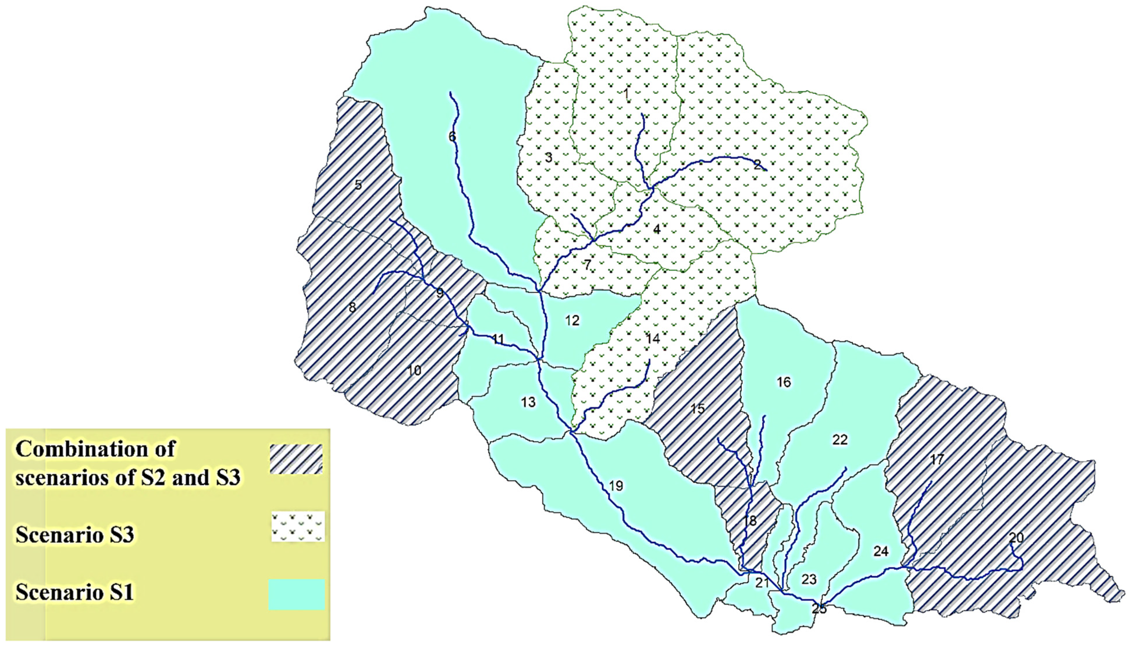
| S1 | S2 | S3 |
|---|---|---|
| No BMPs have been applied in the sub-basins | Application of vegetated filter strips with a width of 5 m in sub-basins and the land use of the orchard, irrigated, and pasture lands | Reduction of fertilizer by 50% in sub-basins and the land use of the orchard and irrigated lands |
| No. | Number of Applied BMPs | Output Nitrate Concentration (mg/L) | Subbasins Under the S2 | Subbasins Under the S3 |
|---|---|---|---|---|
| 1 | 13 | 13.75 | 20/17/9 | 20/9/8/7/5/4/2 |
| 2 | 12 | 13.84 | 18/15/9/5 | 20/15/8/7/3/2 |
| 3 | 7 | 14.25 | 20/5/2 | 9/7/5/4 |
| 4 | 6 | 14.34 | 20/15/14/2/1 | 8/5/1 |
| 5 | 14 | 13.69 | 18/15/9/8/4/2 | 20/9/8/7/5/4/2 |
| 6 | 11 | 13.92 | 18/14/7/3/4/2 | 20/9/8/7/5/4/2 |
| 7 | 2 | 14.91 | 5 | 2 |
| 8 | 18 | 13.67 | 18/7 | 20/9 |
| 9 | 4 | 14.71 | 20/15/14/2/1 | 9/7/5/4 |
| 10 | 10 | 14.04 | 9/7/4/3/1 | 20/5 |
| 11 | 5 | 14.41 | 14/7/4/3 | 10/9/8/5 |
| 12 | 8 | 14.106 | 20/18/5 | 15/14/2/1 |
| 13 | 9 | 14.092 | 3/1 | 9/7/5/4 |
Disclaimer/Publisher’s Note: The statements, opinions and data contained in all publications are solely those of the individual author(s) and contributor(s) and not of MDPI and/or the editor(s). MDPI and/or the editor(s) disclaim responsibility for any injury to people or property resulting from any ideas, methods, instructions or products referred to in the content. |
© 2023 by the authors. Licensee MDPI, Basel, Switzerland. This article is an open access article distributed under the terms and conditions of the Creative Commons Attribution (CC BY) license (https://creativecommons.org/licenses/by/4.0/).
Share and Cite
Hashemi Aslani, Z.; Nasiri, V.; Maftei, C.; Vaseashta, A. Synergetic Integration of SWAT and Multi-Objective Optimization Algorithms for Evaluating Efficiencies of Agricultural Best Management Practices to Improve Water Quality. Land 2023, 12, 401. https://doi.org/10.3390/land12020401
Hashemi Aslani Z, Nasiri V, Maftei C, Vaseashta A. Synergetic Integration of SWAT and Multi-Objective Optimization Algorithms for Evaluating Efficiencies of Agricultural Best Management Practices to Improve Water Quality. Land. 2023; 12(2):401. https://doi.org/10.3390/land12020401
Chicago/Turabian StyleHashemi Aslani, Zohreh, Vahid Nasiri, Carmen Maftei, and Ashok Vaseashta. 2023. "Synergetic Integration of SWAT and Multi-Objective Optimization Algorithms for Evaluating Efficiencies of Agricultural Best Management Practices to Improve Water Quality" Land 12, no. 2: 401. https://doi.org/10.3390/land12020401