


A Fusion of Geothermal and InSAR Data with Machine Learning for Enhanced Deformation Forecasting at the Geysers


Abstract
:Simple Summary
Abstract
1. Introduction
2. Materials and Methods
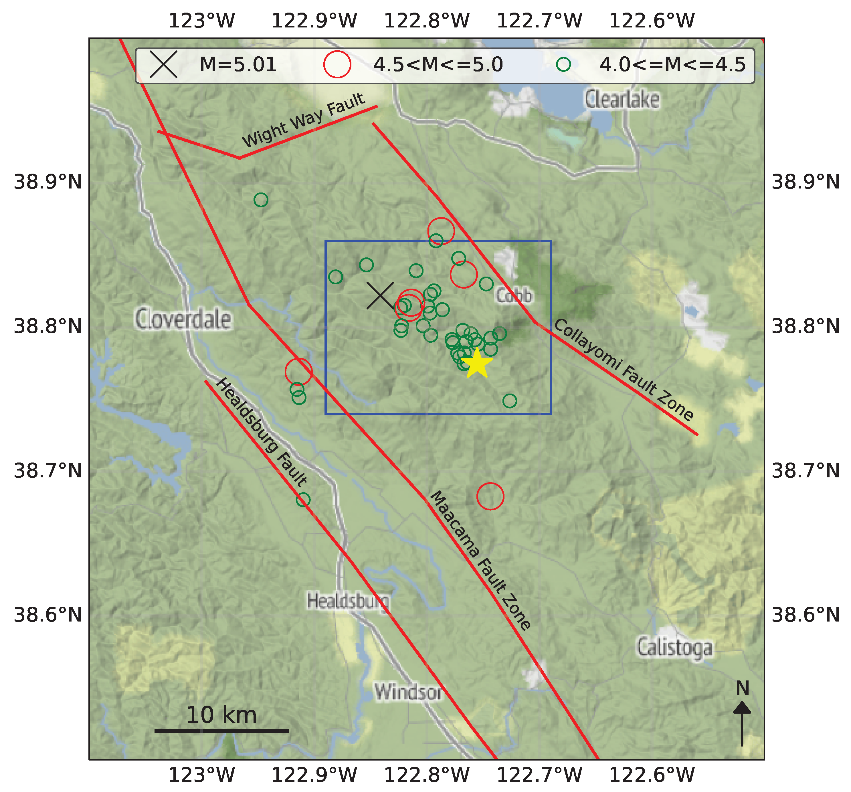
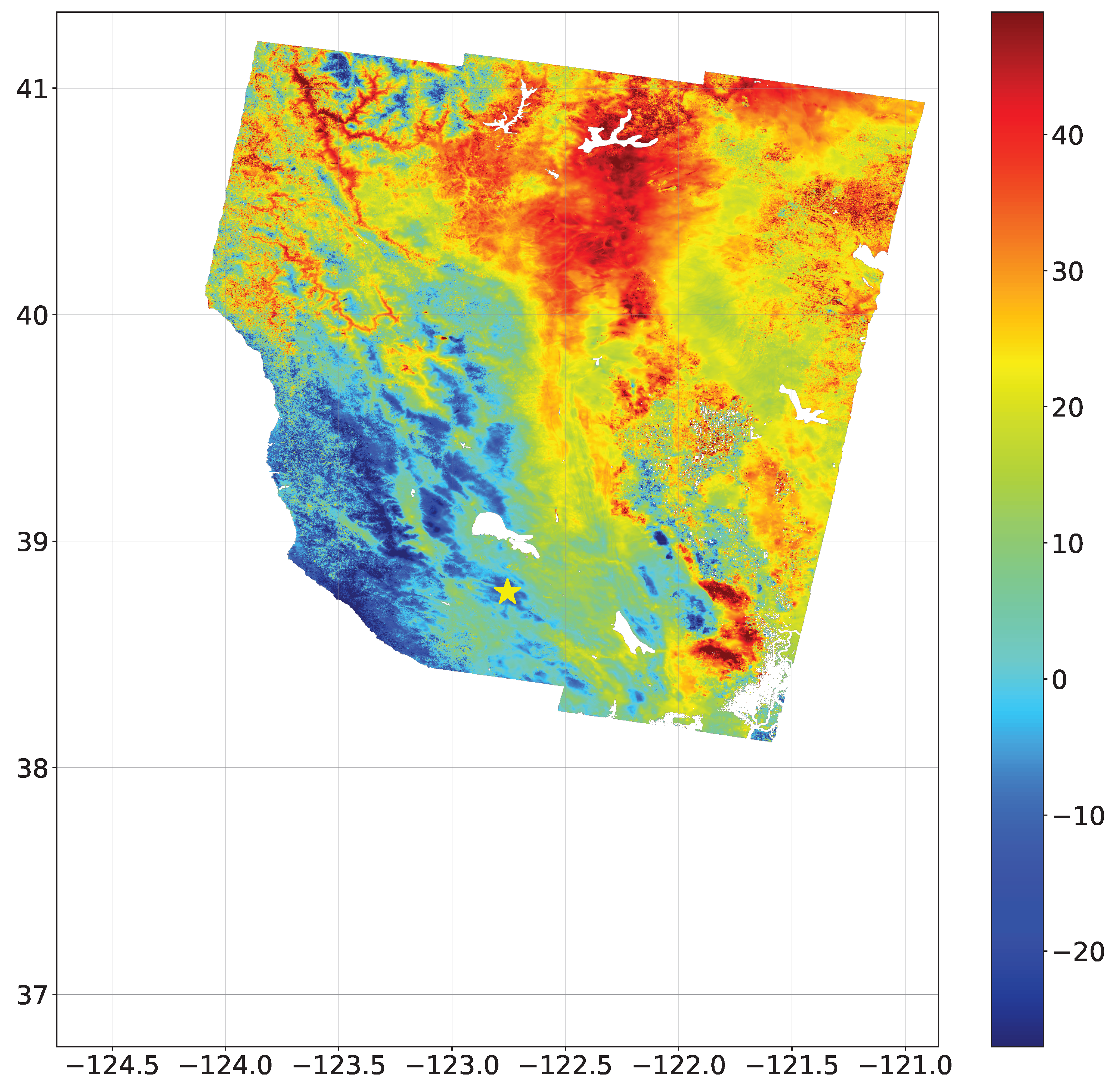
2.1. Area of Study
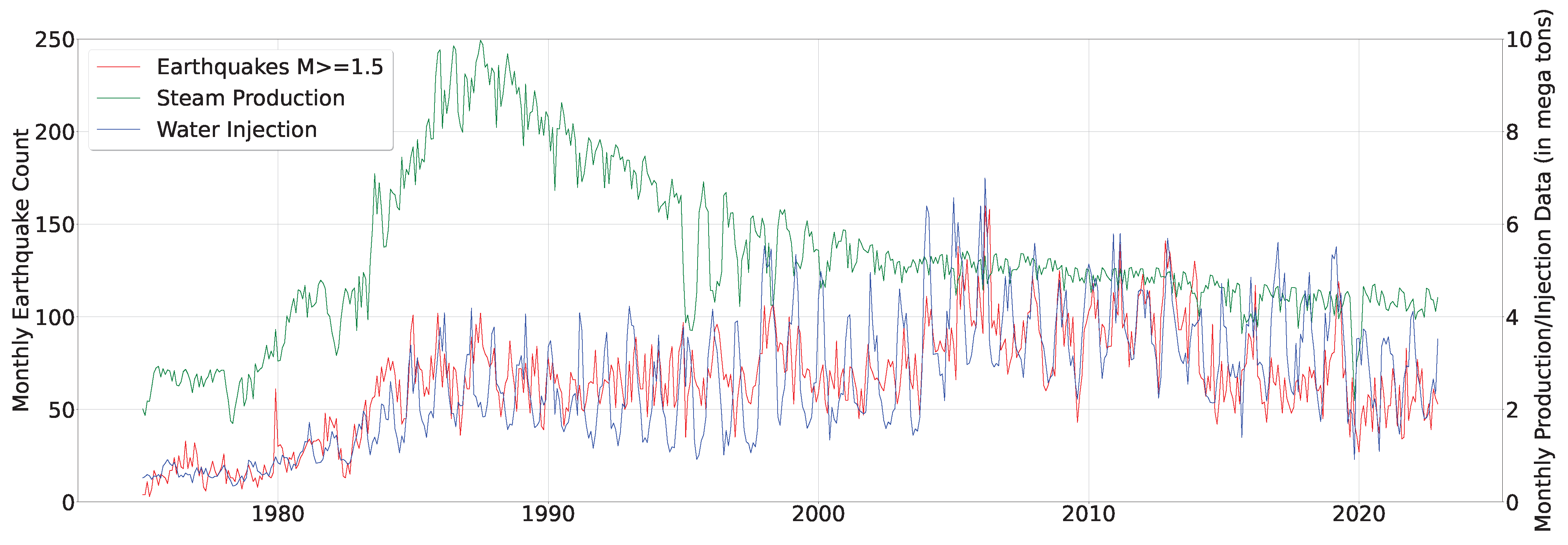
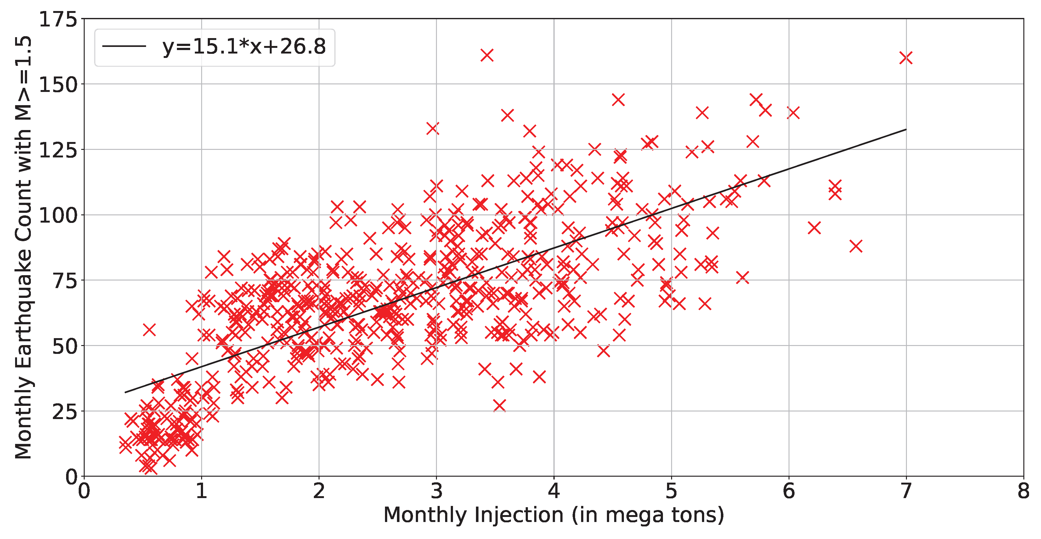
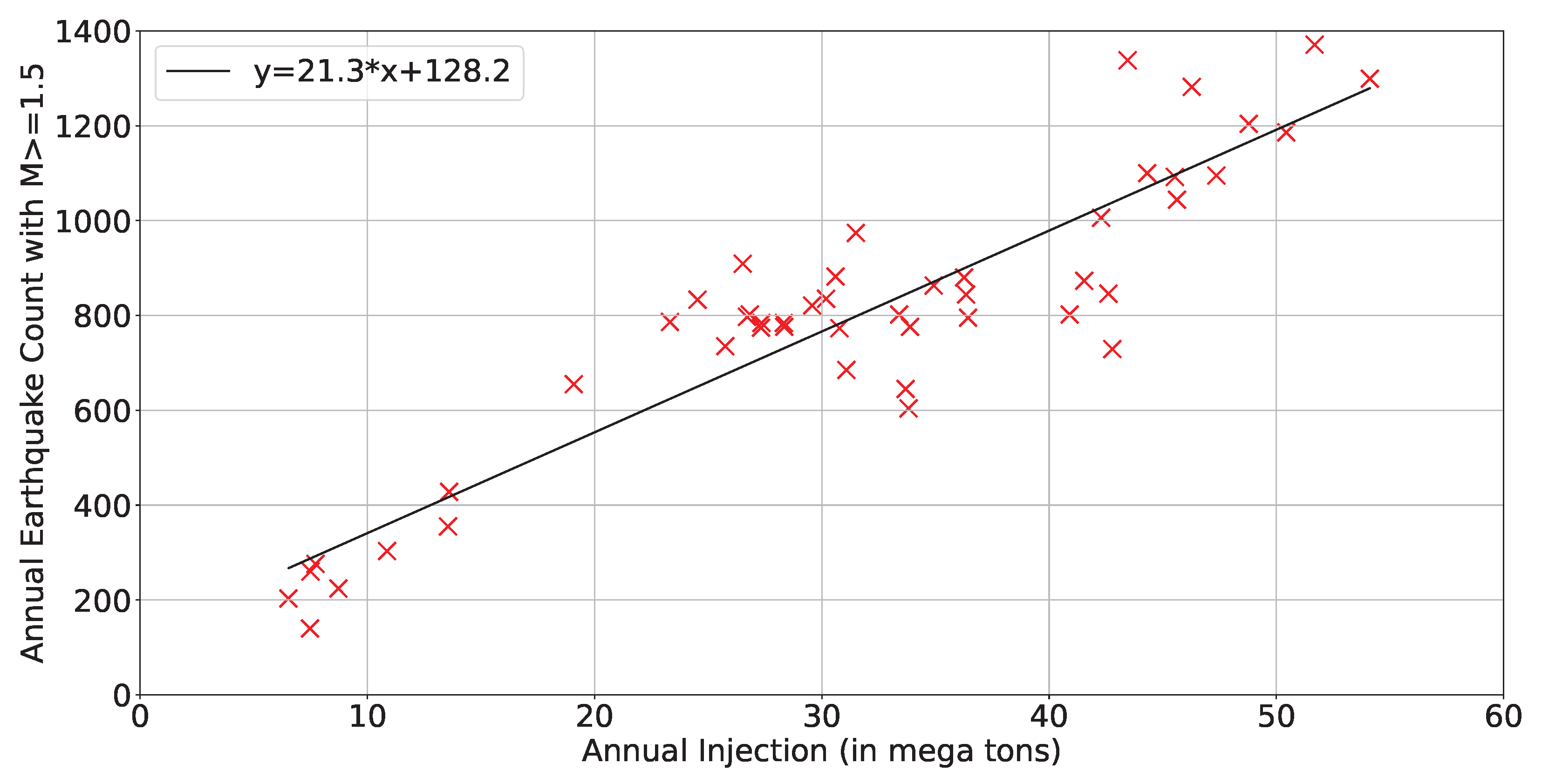
2.2. Correlation Study
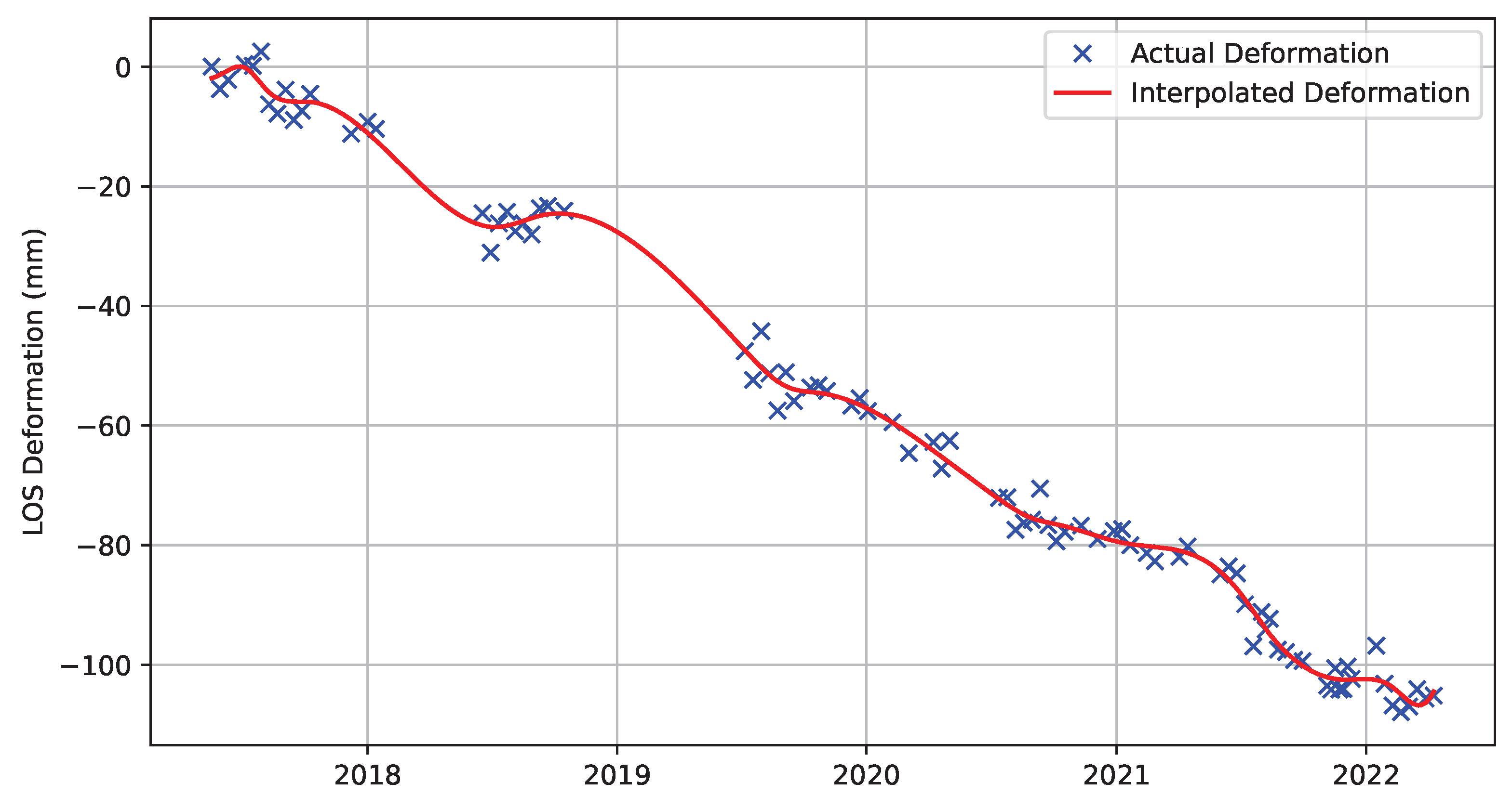
2.3. Data Preprocessing and Baseline Model
- It was not equally temporally separated.
- It had a couple large temporal gaps.
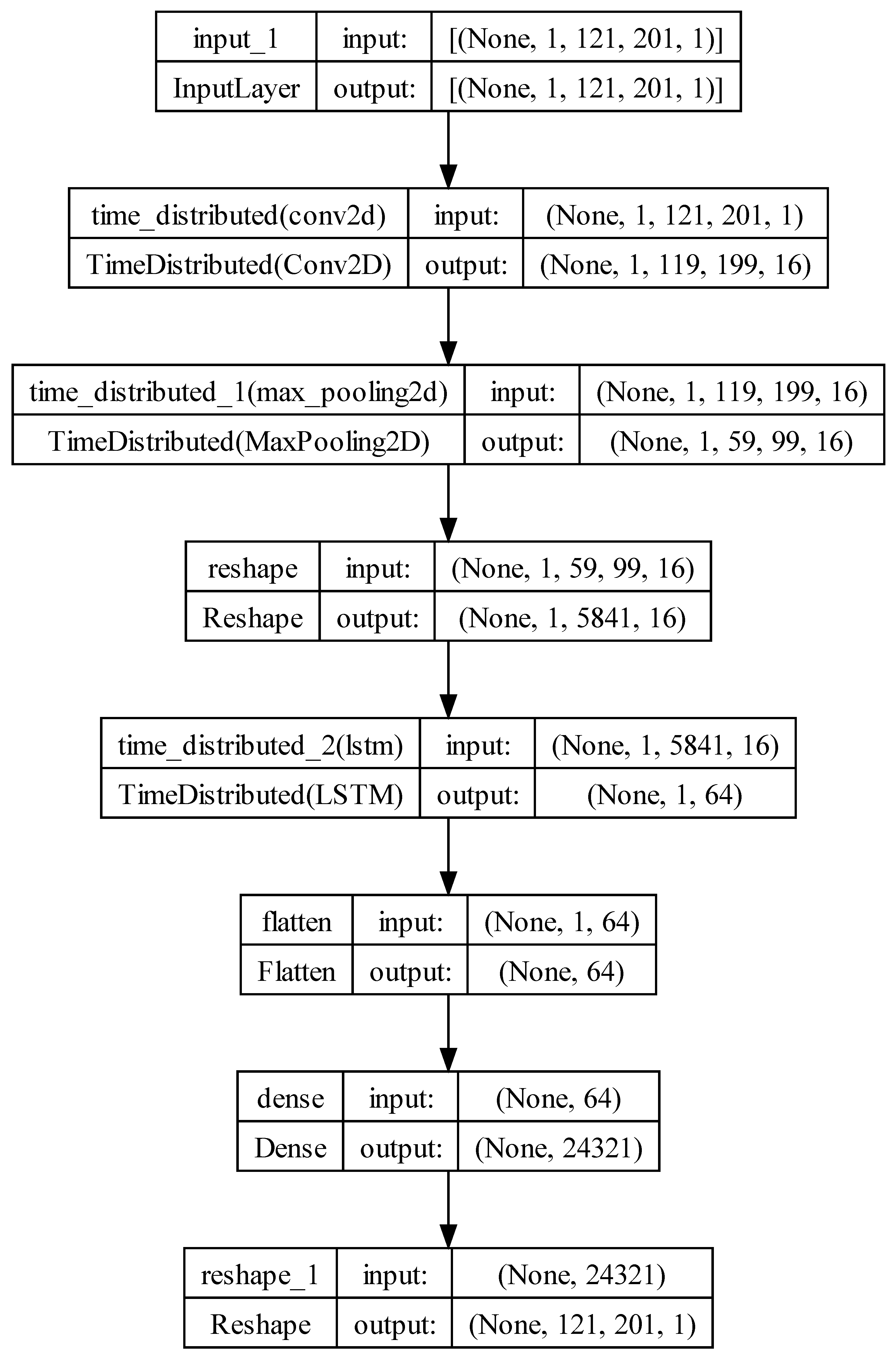
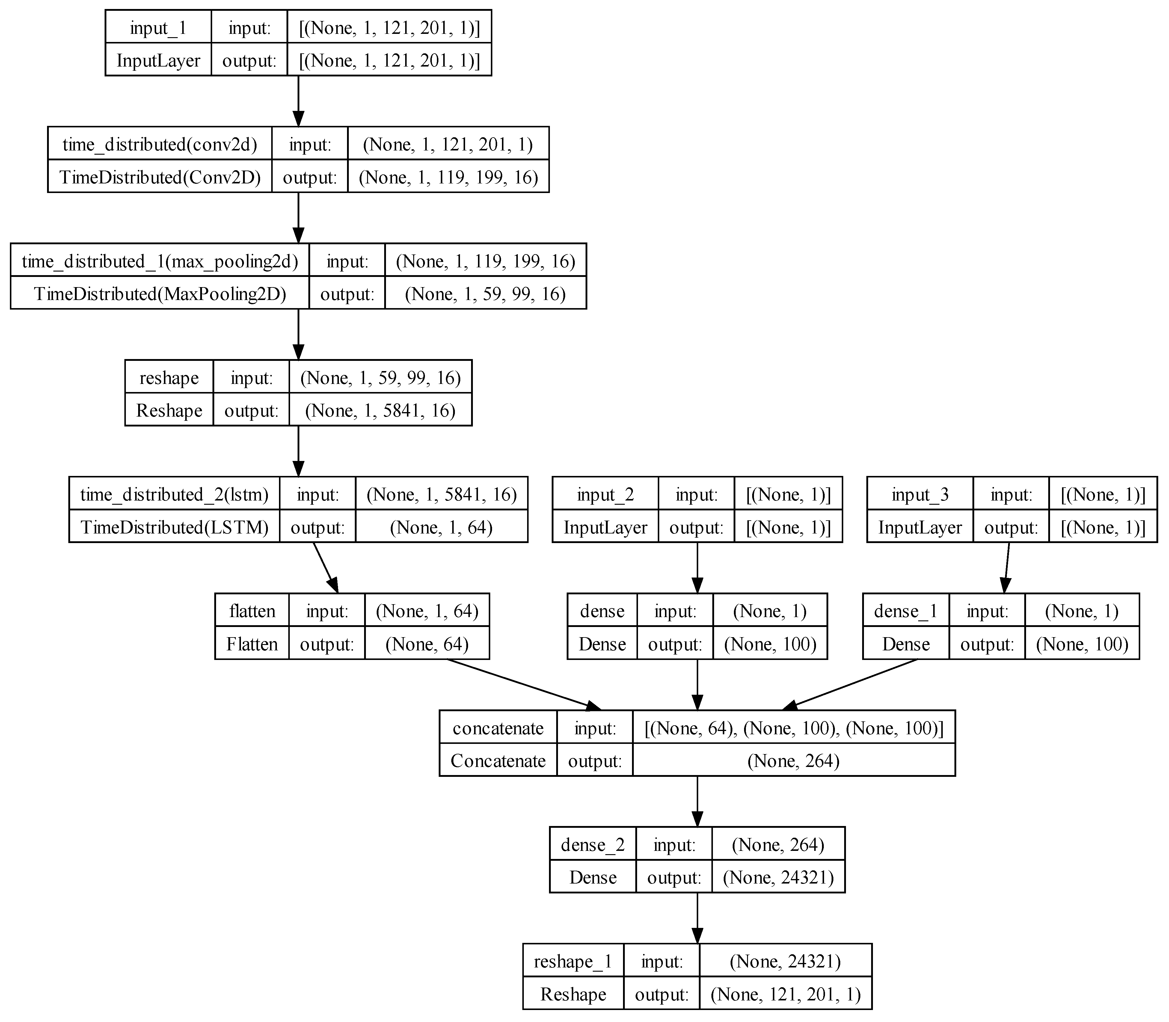
2.4. Machine Learning Models
3. Results
3.1. Correlation Results
3.2. Machine Learning Results
4. Discussion
4.1. Correlation and Machine Learning
4.2. Limitations
4.3. Recommendations
5. Conclusions
Author Contributions
Funding
Data Availability Statement
Acknowledgments
Conflicts of Interest
Abbreviations
| InSAR | Interferometric synthetic aperture radar |
| CNN | Convolutional neural network |
| LSTM | Long short-term memory |
| LOS | Line of sight |
| MSE | Mean squared error |
| GACOS | Generic Atmospheric Correction Online Service for InSAR |
| EGS | Enhanced Geothermal System |
| USGS | United States Geological Survey |
| ML | Machine learning |
| GNSS | Global Navigation Satellite System |
References
- Bommer, J.J.; Crowley, H.; Pinho, R. A risk-mitigation approach to the management of induced seismicity. J. Seismol. 2015, 19, 623–646. [Google Scholar]
- Keranen, K.M.; Weingarten, M. Induced seismicity. Annu. Rev. Earth Planet. Sci. 2018, 46, 149–174. [Google Scholar]
- Kisslinger, C. A review of theories of mechanisms of induced seismicity. Eng. Geol. 1976, 10, 85–98. [Google Scholar]
- Simpson, D.W.; Leith, W.; Scholz, C. Two types of reservoir-induced seismicity. Bull. Seismol. Soc. Am. 1988, 78, 2025–2040. [Google Scholar]
- Norris, J.Q.; Turcotte, D.L.; Moores, E.M.; Brodsky, E.E.; Rundle, J.B. Fracking in tight shales: What is it, what does it accomplish, and what are its consequences? Annu. Rev. Earth Planet. Sci. 2016, 44, 321–351. [Google Scholar] [CrossRef]
- Maury, V.; Grassob, J.R.; Wittlinger, G. Monitoring of subsidence and induced seismicity in the Lacq gas field (France): The consequences on gas production and field operation. Eng. Geol. 1992, 32, 123–135. [Google Scholar]
- Van Thienen-Visser, K.; Breunese, J. Induced seismicity of the Groningen gas field: History and recent developments. Lead. Edge 2015, 34, 664–671. [Google Scholar]
- Hasegawa, H.S.; Wetmiller, R.J.; Gendzwill, D.J. Induced seismicity in mines in Canada—An overview. Pure Appl. Geophys. 1989, 129, 423–453. [Google Scholar]
- Mirek, K.; Mirek, J. Correlation between ground subsidence and induced mining seismicity, Upper Silesia Coal Basin case study. Pol. J. Environ. Stud. 2011, 20, 253–257. [Google Scholar]
- Hejmanowski, R.; Witkowski, W.T.; Guzy, A.; Malinowska, A. Identification of the ground movements caused by mining-induced seismicity with the satellite interferometry. Proc. Int. Assoc. Hydrol. Sci. 2020, 382, 297–301. [Google Scholar] [CrossRef]
- Deng, F.; Dixon, T.H.; Xie, S. Surface deformation and induced seismicity due to fluid injection and oil and gas extraction in western Texas. J. Geophys. Res. Solid Earth 2020, 125, e2019JB018962. [Google Scholar]
- Perski, Z. Applicability of ERS-1 and ERS-2 InSAR for land subsidence monitoring in the Silesian coal mining region, Poland. Int. Arch. Photogramm. Remote Sens. 1998, 32, 555–558. [Google Scholar]
- Holzer, T.L.; Galloway, D.L. Impacts of land subsidence caused by withdrawal of underground fluids in the United States. In Humans as Geologic Agents; Geological Society of America: McLean, VA, USA, 2005. [Google Scholar]
- Xue, Y.Q.; Zhang, Y.; Ye, S.J.; Wu, J.C.; Li, Q.F. Land subsidence in China. Environ. Geol. 2005, 48, 713–720. [Google Scholar]
- Ishwar, S.; Kumar, D. Application of DInSAR in mine surface subsidence monitoring and prediction. Curr. Sci. 2017, 112, 46–51. [Google Scholar] [CrossRef]
- Hill, D.P.; Eaton, J.P.; Jones, L.M. Seismicity, 1980-86. U. S. Geol. Surv. Prof. Pap. 1990, 1515. Available online: https://www.osti.gov/biblio/5599608 (accessed on 19 September 2023).
- Henderson, J.; Barton, D.; Foulger, G. Fractal clustering of induced seismicity in The Geysers geothermal area, California. Geophys. J. Int. 1999, 139, 317–324. [Google Scholar]
- Eberhart-Phillips, D.; Oppenheimer, D.H. Induced seismicity in The Geysers geothermal area, California. J. Geophys. Res. Solid Earth 1984, 89, 1191–1207. [Google Scholar] [CrossRef]
- Ludwin, R.; Bufe, C. Continued Seismic Monitoring of The Geysers, California Geothermal Area; Technical Report; Geological Survey: Washington, DC, USA, 1980. [Google Scholar]
- Stark, M.A. Microearthquakes—A tool to track injected water in The Geysers reservoir. Monogr. Geyser Geotherm. Field Spec. Rep. 1992, 17, 111–117. [Google Scholar]
- Majer, E.L.; Baria, R.; Stark, M.; Oates, S.; Bommer, J.; Smith, B.; Asanuma, H. Induced seismicity associated with enhanced geothermal systems. Geothermics 2007, 36, 185–222. [Google Scholar]
- Hamilton, R.; Muffler, L. Microearthquakes at the Geysers geothermal area, California. J. Geophys. Res. 1972, 77, 2081–2086. [Google Scholar] [CrossRef]
- Shakibay Senobari, N.; Funning, G.J. Widespread fault creep in the northern San Francisco Bay Area revealed by multistation cluster detection of repeating earthquakes. Geophys. Res. Lett. 2019, 46, 6425–6434. [Google Scholar] [CrossRef]
- Field, E.H.; Arrowsmith, R.J.; Biasi, G.P.; Bird, P.; Dawson, T.E.; Felzer, K.R.; Jackson, D.D.; Johnson, K.M.; Jordan, T.H.; Madden, C.; et al. Uniform California earthquake rupture forecast, version 3 (UCERF3)—The time-independent model. Bull. Seismol. Soc. Am. 2014, 104, 1122–1180. [Google Scholar] [CrossRef]
- Luginbuhl, M.; Rundle, J.B.; Hawkins, A.; Turcotte, D.L. Nowcasting earthquakes: A comparison of induced earthquakes in Oklahoma and at the Geysers, California. Pure Appl. Geophys. 2018, 175, 49–65. [Google Scholar] [CrossRef]
- Vasco, D.; Rutqvist, J.; Ferretti, A.; Rucci, A.; Bellotti, F.; Dobson, P.; Oldenburg, C.; Garcia, J.; Walters, M.; Hartline, C. Monitoring deformation at the Geysers Geothermal Field, California using C-band and X-band interferometric synthetic aperture radar. Geophys. Res. Lett. 2013, 40, 2567–2572. [Google Scholar] [CrossRef]
- Lofgren, B.; McLaughlin, R.; Donnelly-Nolan, J. Monitoring crustal deformation in The Geysers-Clear Lake region. US Geol. Surv. Prof. Pap 1981, 1141, 139–148. [Google Scholar]
- Mossop, A.; Segall, P. Subsidence at The Geysers geothermal field, N. California from a comparison of GPS and leveling surveys. Geophys. Res. Lett. 1997, 24, 1839–1842. [Google Scholar] [CrossRef]
- Sarychikhina, O.; Glowacka, E.; Mellors, R.; Vidal, F.S. Land subsidence in the Cerro Prieto Geothermal Field, Baja California, Mexico, from 1994 to 2005: An integrated analysis of DInSAR, leveling and geological data. J. Volcanol. Geotherm. Res. 2011, 204, 76–90. [Google Scholar] [CrossRef]
- Allis, R.; Bromley, C.; Currie, S. Update on subsidence at the Wairakei–Tauhara geothermal system, New Zealand. Geothermics 2009, 38, 169–180. [Google Scholar] [CrossRef]
- White, P.J.; Lawless, J.V.; Terzaghi, S.; Okada, W. Advances in subsidence modelling of exploited geothermal fields. In Proceedings of the World Geothermal Congress 2005, Antalya, Turkey, 24–29 April 2005; pp. 24–29. [Google Scholar]
- Chen, S.; Zhang, Q.; Andrews-Speed, P.; Mclellan, B. Quantitative assessment of the environmental risks of geothermal energy: A review. J. Environ. Manag. 2020, 276, 111287. [Google Scholar]
- Deichmann, N.; Giardini, D. Earthquakes induced by the stimulation of an enhanced geothermal system below Basel (Switzerland). Seismol. Res. Lett. 2009, 80, 784–798. [Google Scholar] [CrossRef]
- Baisch, S.; Carbon, D.; Dannwolf, U.; Delacou, B.; Devaux, M.; Dunand, F.; Jung, R.; Koller, M.; Martin, C.; Sartori, M.; et al. Deep Heat Mining Basel: Seismic Risk Analysis; SERIANEX Group, Departement für Wirtschaft, Soziales und Umwelt des Kantons Basel-Stadt: Basel, Switzerland, 2009. [Google Scholar]
- McClure, M.W.; Horne, R.N. An investigation of stimulation mechanisms in Enhanced Geothermal Systems. Int. J. Rock Mech. Min. Sci. 2014, 72, 242–260. [Google Scholar]
- Olasolo, P.; Juárez, M.; Morales, M.; Liarte, I. Enhanced geothermal systems (EGS): A review. Renew. Sustain. Energy Rev. 2016, 56, 133–144. [Google Scholar]
- Nielson, D.; Moore, J. The deeper parts of the geysers thermal system-hviplications for heat recovery. In Proceedings of the World Geothermal Congress 2000, Kyushu-Tohoku, Japan, 28 May–10 June 2000. [Google Scholar]
- Garcia, J.; Hartline, C.; Walters, M.; Wright, M.; Rutqvist, J.; Dobson, P.F.; Jeanne, P. The Northwest Geysers EGS demonstration project, California: Part 1: Characterization and reservoir response to injection. Geothermics 2016, 63, 97–119. [Google Scholar]
- Garcia, J.; Walters, M.; Beall, J.; Hartline, C.; Pingol, A.; Pistone, S.; Wright, M. Overview of the northwest Geysers EGS demonstration project. In Proceedings of the Thirty-Seventh Workshop on Geothermal Reservoir Engineering 2012, Stanford, CA, USA, 30 January–1 February 2012; Volume 30. [Google Scholar]
- Hartline, C.; Walters, M.; Wright, M.; Rawal, C.; Garcia, J.; Farison, J. The Northwest Geysers Enhanced Geothermal System Demonstration Project, The Geysers, California. Final Report; Technical Report; Geysers Power Company, LLC: Houston, TX, USA, 2019. [Google Scholar]
- Hu, B.; Chen, J.; Zhang, X. Monitoring the land subsidence area in a coastal urban area with InSAR and GNSS. Sensors 2019, 19, 3181. [Google Scholar] [PubMed]
- Bürgmann, R.; Rosen, P.A.; Fielding, E.J. Synthetic aperture radar interferometry to measure Earth’s surface topography and its deformation. Annu. Rev. Earth Planet. Sci. 2000, 28, 169–209. [Google Scholar]
- Massonnet, D.; Feigl, K.L. Radar interferometry and its application to changes in the Earth’s surface. Rev. Geophys. 1998, 36, 441–500. [Google Scholar]
- Pepe, A.; Calò, F. A review of interferometric synthetic aperture RADAR (InSAR) multi-track approaches for the retrieval of Earth’s surface displacements. Appl. Sci. 2017, 7, 1264. [Google Scholar] [CrossRef]
- Smith, L.C. Emerging applications of interferometric synthetic aperture radar (InSAR) in geomorphology and hydrology. Ann. Assoc. Am. Geogr. 2002, 92, 385–398. [Google Scholar] [CrossRef]
- Torres, R.; Snoeij, P.; Geudtner, D.; Bibby, D.; Davidson, M.; Attema, E.; Potin, P.; Rommen, B.; Floury, N.; Brown, M.; et al. GMES Sentinel-1 mission. Remote Sens. Environ. 2012, 120, 9–24. [Google Scholar]
- Geudtner, D.; Torres, R.; Snoeij, P.; Davidson, M.; Rommen, B. Sentinel-1 system capabilities and applications. In Proceedings of the 2014 IEEE Geoscience and Remote Sensing Symposium, Quebec City, QC, Canada, 13–18 July 2014; pp. 1457–1460. [Google Scholar]
- Hole, J.; Bromley, C.; Stevens, N.; Wadge, G. Subsidence in the geothermal fields of the Taupo Volcanic Zone, New Zealand from 1996 to 2005 measured by InSAR. J. Volcanol. Geotherm. Res. 2007, 166, 125–146. [Google Scholar]
- Békési, E.; Fokker, P.A.; Martins, J.E.; Limberger, J.; Bonté, D.; Van Wees, J.D. Production-induced subsidence at the Los Humeros geothermal field inferred from PS-InSAR. Geofluids 2019, 2019, 2306092. [Google Scholar]
- Benos, L.; Tagarakis, A.C.; Dolias, G.; Berruto, R.; Kateris, D.; Bochtis, D. Machine learning in agriculture: A comprehensive updated review. Sensors 2021, 21, 3758. [Google Scholar] [PubMed]
- Dixon, M.F.; Halperin, I.; Bilokon, P. Machine Learning in Finance; Springer: Berlin/Heidelberg, Germany, 2020; Volume 1170. [Google Scholar]
- Rajkomar, A.; Dean, J.; Kohane, I. Machine learning in medicine. N. Engl. J. Med. 2019, 380, 1347–1358. [Google Scholar] [CrossRef] [PubMed]
- Mahesh, B. Machine learning algorithms-a review. Int. J. Sci. Res. (IJSR) 2020, 9, 381–386. [Google Scholar]
- Brengman, C.M.; Barnhart, W.D. Identification of surface deformation in InSAR using machine learning. Geochem. Geophys. Geosyst. 2021, 22, e2020GC009204. [Google Scholar]
- Anantrasirichai, N.; Biggs, J.; Albino, F.; Hill, P.; Bull, D. Application of machine learning to classification of volcanic deformation in routinely generated InSAR data. J. Geophys. Res. Solid Earth 2018, 123, 6592–6606. [Google Scholar]
- Xie, Z.; Chen, G.; Meng, X.; Zhang, Y.; Qiao, L.; Tan, L. A comparative study of landslide susceptibility mapping using weight of evidence, logistic regression and support vector machine and evaluated by SBAS-InSAR monitoring: Zhouqu to Wudu segment in Bailong River Basin, China. Environ. Earth Sci. 2017, 76, 1–19. [Google Scholar]
- Rongier, G.; Rude, C.; Herring, T.; Pankratius, V. Generative modeling of InSAR interferograms. Earth Space Sci. 2019, 6, 2671–2683. [Google Scholar]
- Roberts, S.; Delorey, A.; Johnson, C.W.; Guyer, R.; Alfaro-Diaz, R.; Johnson, P. Using surface deformation and machine learning to determine state of stress changes at the coso geothermal field, california USA. In Proceedings of the 46th Workshop on Geothermal Reservoir Engineering, Stanford, CA, USA, 15–17 February 2021. [Google Scholar]
- Cavur, M.; Moraga, J.; Duzgun, H.S.; Soydan, H.; Jin, G. The DInSAR Analysis with Machine Learning for Delineating Geothermal Sites at the Brady Geothermal Field. In Proceedings of the 46th Workshop on Geothermal Reservoir Engineering, Stanford, CA, USA, 15–17 February 2021. [Google Scholar]
- Holtzman, B.K.; Paté, A.; Paisley, J.; Waldhauser, F.; Repetto, D. Machine learning reveals cyclic changes in seismic source spectra in Geysers geothermal field. Sci. Adv. 2018, 4, eaao2929. [Google Scholar] [CrossRef]
- Prezioso, E.; Sharma, N.; Piccialli, F.; Convertito, V. A data-driven artificial neural network model for the prediction of ground motion from induced seismicity: The case of The Geysers geothermal field. Front. Earth Sci. 2022, 10, 917608. [Google Scholar] [CrossRef]
- Khan, M.A.; Truschel, J. The Geysers geothermal field, an injection success story. GRC Trans. 2010, 34, 1239–1242. [Google Scholar]
- Thomas, R.P. Heat-Flow Mapping at The Geysers Geothermal Field; Technical Report; California Department of Conservation: Sacramento, CA, USA, 1986. [Google Scholar]
- Lin, G.; Wu, B. Seismic velocity structure and characteristics of induced seismicity at the Geysers geothermal field, eastern California. Geothermics 2018, 71, 225–233. [Google Scholar] [CrossRef]
- Ranalli, G.; Rybach, L. Heat flow, heat transfer and lithosphere rheology in geothermal areas: Features and examples. J. Volcanol. Geotherm. Res. 2005, 148, 3–19. [Google Scholar] [CrossRef]
- Mitchell, M.A.; Peacock, J.R.; Burgess, S.D. Imaging the magmatic plumbing of the Clear Lake Volcanic Field using 3-D gravity inversions. J. Volcanol. Geotherm. Res. 2023, 435, 107758. [Google Scholar]
- Kwiatek, G.; Martínez-Garzón, P.; Dresen, G.; Bohnhoff, M.; Sone, H.; Hartline, C. Effects of long-term fluid injection on induced seismicity parameters and maximum magnitude in northwestern part of The Geysers geothermal field. J. Geophys. Res. Solid Earth 2015, 120, 7085–7101. [Google Scholar] [CrossRef]
- Majer, E.L.; Peterson, J.E. The impact of injection on seismicity at The Geysers, California Geothermal Field. Int. J. Rock Mech. Min. Sci. 2007, 44, 1079–1090. [Google Scholar]
- Martínez-Garzón, P.; Bohnhoff, M.; Kwiatek, G.; Dresen, G. Stress tensor changes related to fluid injection at The Geysers geothermal field, California. Geophys. Res. Lett. 2013, 40, 2596–2601. [Google Scholar] [CrossRef]
- Sanyal, S.K. Forty years of production history at the geysers geothermal field, California—The lessons learned. Geotherm. Resour. Counc. Trans. 2000, 24, 317–323. [Google Scholar]
- Sanyal, S.K.; Enedy, S.L. Fifty years of power generation at the Geysers geothermal field, California—The lessons learned. In Proceedings of the 36th Workshop on Geothermal Reservoir Engineering, Stanford, CA, USA, 31 January–2 February 2011. [Google Scholar]
- Chaussard, E.; Wdowinski, S.; Cabral-Cano, E.; Amelung, F. Land subsidence in central Mexico detected by ALOS InSAR time-series. Remote Sens. Environ. 2014, 140, 94–106. [Google Scholar]
- Aljammaz, A.; Sultan, M.; Izadi, M.; Abotalib, A.Z.; Elhebiry, M.S.; Emil, M.K.; Abdelmohsen, K.; Saleh, M.; Becker, R. Land subsidence induced by rapid urbanization in arid environments: A remote sensing-based investigation. Remote Sens. 2021, 13, 1109. [Google Scholar] [CrossRef]
- Jin, B.; Yin, K.; Li, Q.; Gui, L.; Yang, T.; Zhao, B.; Guo, B.; Zeng, T.; Ma, Z. Susceptibility analysis of land subsidence along the transmission line in the salt lake area based on remote sensing interpretation. Remote Sens. 2022, 14, 3229. [Google Scholar] [CrossRef]
- Bagheri-Gavkosh, M.; Hosseini, S.M.; Ataie-Ashtiani, B.; Sohani, Y.; Ebrahimian, H.; Morovat, F.; Ashrafi, S. Land subsidence: A global challenge. Sci. Total Environ. 2021, 778, 146193. [Google Scholar]
- Scudiero, E.; Skaggs, T.H.; Corwin, D.L. Regional scale soil salinity evaluation using Landsat 7, western San Joaquin Valley, California, USA. Geoderma Reg. 2014, 2, 82–90. [Google Scholar] [CrossRef]
- Cohen, I.; Huang, Y.; Chen, J.; Benesty, J.; Benesty, J.; Chen, J.; Huang, Y.; Cohen, I. Pearson correlation coefficient. In Noise Reduction in Speech Processing; Springer: Berlin/Heidelberg, Germany, 2009; pp. 1–4. [Google Scholar]
- Chok, N.S. Pearson’s Versus Spearman’s and Kendall’s Correlation Coefficients for Continuous Data. Ph.D. Thesis, University of Pittsburgh, Pittsburgh, PA, USA, 2010. [Google Scholar]
- Gupta, S.; Kapoor, V. Fundamentals of Mathematical Statistics; Sultan Chand & Sons: New Delhi, India, 2020. [Google Scholar]
- Hauke, J.; Kossowski, T. Comparison of values of Pearson’s and Spearman’s correlation coefficients on the same sets of data. Quaest. Geogr. 2011, 30, 87–93. [Google Scholar] [CrossRef]
- Morishita, Y.; Lazecky, M.; Wright, T.J.; Weiss, J.R.; Elliott, J.R.; Hooper, A. LiCSBAS: An open-source InSAR time series analysis package integrated with the LiCSAR automated Sentinel-1 InSAR processor. Remote Sens. 2020, 12, 424. [Google Scholar] [CrossRef]
- Morishita, Y. Nationwide urban ground deformation monitoring in Japan using Sentinel-1 LiCSAR products and LiCSBAS. Prog. Earth Planet. Sci. 2021, 8, 1–23. [Google Scholar]
- Lazeckỳ, M.; Spaans, K.; González, P.J.; Maghsoudi, Y.; Morishita, Y.; Albino, F.; Elliott, J.; Greenall, N.; Hatton, E.; Hooper, A.; et al. LiCSAR: An automatic InSAR tool for measuring and monitoring tectonic and volcanic activity. Remote Sens. 2020, 12, 2430. [Google Scholar] [CrossRef]
- Wright, T.; Gonzalez, P.; Walters, R.; Hatton, E.; Spaans, K.; Hooper, A. LiCSAR: Tools for automated generation of Sentinel-1 frame interferograms. In Proceedings of the AGU Fall Meeting Abstracts 2016, San Francisco, CA, USA, 12–16 December 2016; Volume 2016, p. G23A-1037. [Google Scholar]
- Lawrence, B.N.; Bennett, V.L.; Churchill, J.; Juckes, M.; Kershaw, P.; Pascoe, S.; Pepler, S.; Pritchard, M.; Stephens, A. Storing and manipulating environmental big data with JASMIN. In Proceedings of the 2013 IEEE International Conference on Big Data, Santa Clara, CA, USA, 6–9 October 2013; pp. 68–75. [Google Scholar]
- Yu, C.; Li, Z.; Penna, N.T.; Crippa, P. Generic atmospheric correction model for interferometric synthetic aperture radar observations. J. Geophys. Res. Solid Earth 2018, 123, 9202–9222. [Google Scholar] [CrossRef]
- Yu, C.; Li, Z.; Penna, N.T. Interferometric synthetic aperture radar atmospheric correction using a GPS-based iterative tropospheric decomposition model. Remote Sens. Environ. 2018, 204, 109–121. [Google Scholar] [CrossRef]
- Yu, C.; Penna, N.T.; Li, Z. Generation of real-time mode high-resolution water vapor fields from GPS observations. J. Geophys. Res. Atmos. 2017, 122, 2008–2025. [Google Scholar] [CrossRef]
- Yu, C.; Li, Z.; Penna, N.T. Triggered afterslip on the southern Hikurangi subduction interface following the 2016 Kaikōura earthquake from InSAR time series with atmospheric corrections. Remote Sens. Environ. 2020, 251, 112097. [Google Scholar]
- Wu, R.; Hamshaw, S.D.; Yang, L.; Kincaid, D.W.; Etheridge, R.; Ghasemkhani, A. Data imputation for multivariate time series sensor data with large gaps of missing data. IEEE Sens. J. 2022, 22, 10671–10683. [Google Scholar]
- Virtanen, P.; Gommers, R.; Oliphant, T.E.; Haberland, M.; Reddy, T.; Cournapeau, D.; Burovski, E.; Peterson, P.; Weckesser, W.; Bright, J.; et al. SciPy 1.0: Fundamental Algorithms for Scientific Computing in Python. Nat. Methods 2020, 17, 261–272. [Google Scholar] [CrossRef] [PubMed]
- Zhu, K.; Zhang, X.; Sun, Q.; Wang, H.; Hu, J. Characterizing spatiotemporal patterns of land deformation in the Santa Ana Basin, Los Angeles, from InSAR time series and independent component analysis. Remote Sens. 2022, 14, 2624. [Google Scholar] [CrossRef]
- Filipponi, F. Sentinel-1 GRD preprocessing workflow. In Proceedings of the 3rd International Electronic Conference on Remote Sensing, Online, 22 May–5 June 2019; p. 11. [Google Scholar]
- Pedregosa, F.; Varoquaux, G.; Gramfort, A.; Michel, V.; Thirion, B.; Grisel, O.; Blondel, M.; Prettenhofer, P.; Weiss, R.; Dubourg, V.; et al. Scikit-learn: Machine Learning in Python. J. Mach. Learn. Res. 2011, 12, 2825–2830. [Google Scholar]
- Tang, W.; Li, B.; Tan, S.; Barni, M.; Huang, J. CNN-based adversarial embedding for image steganography. IEEE Trans. Inf. Forensics Secur. 2019, 14, 2074–2087. [Google Scholar]
- Cai, J.; Gu, S.; Zhang, L. Learning a deep single image contrast enhancer from multi-exposure images. IEEE Trans. Image Process. 2018, 27, 2049–2062. [Google Scholar] [CrossRef] [PubMed]
- Zhou, W.; Newsam, S.; Li, C.; Shao, Z. Learning low dimensional convolutional neural networks for high-resolution remote sensing image retrieval. Remote Sens. 2017, 9, 489. [Google Scholar]
- Tang, T.; Zhou, S.; Deng, Z.; Zou, H.; Lei, L. Vehicle detection in aerial images based on region convolutional neural networks and hard negative example mining. Sensors 2017, 17, 336. [Google Scholar]
- Rajagukguk, R.A.; Ramadhan, R.A.; Lee, H.J. A review on deep learning models for forecasting time series data of solar irradiance and photovoltaic power. Energies 2020, 13, 6623. [Google Scholar] [CrossRef]
- Zhao, B.; Lu, H.; Chen, S.; Liu, J.; Wu, D. Convolutional neural networks for time series classification. J. Syst. Eng. Electron. 2017, 28, 162–169. [Google Scholar]
- Gu, J.; Wang, Z.; Kuen, J.; Ma, L.; Shahroudy, A.; Shuai, B.; Liu, T.; Wang, X.; Wang, G.; Cai, J.; et al. Recent advances in convolutional neural networks. Pattern Recognit. 2018, 77, 354–377. [Google Scholar]
- O’Shea, K.; Nash, R. An introduction to convolutional neural networks. arXiv 2015, arXiv:1511.08458. [Google Scholar]
- Hinton, G.E.; Srivastava, N.; Krizhevsky, A.; Sutskever, I.; Salakhutdinov, R.R. Improving neural networks by preventing co-adaptation of feature detectors. arXiv 2012, arXiv:1207.0580. [Google Scholar]
- Albawi, S.; Mohammed, T.A.; Al-Zawi, S. Understanding of a convolutional neural network. In Proceedings of the 2017 International Conference on Engineering and Technology (ICET), Antalya, Turkey, 21–23 August 2017; pp. 1–6. [Google Scholar]
- Karasu, S.; Altan, A. Crude oil time series prediction model based on LSTM network with chaotic Henry gas solubility optimization. Energy 2022, 242, 122964. [Google Scholar]
- Sopelsa Neto, N.F.; Stefenon, S.F.; Meyer, L.H.; Ovejero, R.G.; Leithardt, V.R.Q. Fault prediction based on leakage current in contaminated insulators using enhanced time series forecasting models. Sensors 2022, 22, 6121. [Google Scholar]
- Gers, F.A.; Eck, D.; Schmidhuber, J. Applying LSTM to time series predictable through time-window approaches. In Proceedings of the International Conference on Artificial Neural Networks 2001, Vienna, Austria, 21–25 August 2001; pp. 669–676. [Google Scholar]
- Pathan, R.K.; Biswas, M.; Khandaker, M.U. Time series prediction of COVID-19 by mutation rate analysis using recurrent neural network-based LSTM model. Chaos Solitons Fractals 2020, 138, 110018. [Google Scholar]
- Yu, Y.; Si, X.; Hu, C.; Zhang, J. A review of recurrent neural networks: LSTM cells and network architectures. Neural Comput. 2019, 31, 1235–1270. [Google Scholar]
- Abadi, M.; Barham, P.; Chen, J.; Chen, Z.; Davis, A.; Dean, J.; Devin, M.; Ghemawat, S.; Irving, G.; Isard, M.; et al. {TensorFlow}: A system for {Large-Scale} machine learning. In Proceedings of the 12th USENIX Symposium on Operating Systems Design and Implementation (OSDI 16), Savannah, GA, USA, 2–4 November 2016; pp. 265–283. [Google Scholar]
- Batini, F.; Bertini, G.; Gianelli, G.; Pandeli, E.; Puxeddu, M.; Villa, I. Deep structure, age and evolution of the Larderello-Travale geothermal field. Trans. Geotherm. Resourc. Counc. 1985, 9, 253–259. [Google Scholar]
- Leptokaropoulos, K.; Staszek, M.; Lasocki, S.; Martínez-Garzón, P.; Kwiatek, G. Evolution of seismicity in relation to fluid injection in the North-Western part of The Geysers geothermal field. Geophys. J. Int. 2018, 212, 1157–1166. [Google Scholar]
- Ma, P.; Zhang, F.; Lin, H. Prediction of InSAR time-series deformation using deep convolutional neural networks. Remote Sens. Lett. 2020, 11, 137–145. [Google Scholar] [CrossRef]
- Liu, Q.; Zhang, Y.; Wei, J.; Wu, H.; Deng, M. HLSTM: Heterogeneous long short-term memory network for large-scale InSAR ground subsidence prediction. IEEE J. Sel. Top. Appl. Earth Obs. Remote Sens. 2021, 14, 8679–8688. [Google Scholar] [CrossRef]
- Hill, P.; Biggs, J.; Ponce-López, V.; Bull, D. Time-Series Prediction Approaches to Forecasting Deformation in Sentinel-1 InSAR Data. J. Geophys. Res. Solid Earth 2021, 126, e2020JB020176. [Google Scholar] [CrossRef]
- Yazbeck, J.; Rundle, J.B. Predicting Short-Term Deformation in the Central Valley Using Machine Learning. Remote Sens. 2023, 15, 449. [Google Scholar] [CrossRef]
- Kagan, Y.Y. Accuracy of modern global earthquake catalogs. Phys. Earth Planet. Inter. 2003, 135, 173–209. [Google Scholar] [CrossRef]
- Helffrich, G.R. How good are routinely determined focal mechanisms? Empirical statistics based on a comparison of Harvard, USGS and ERI moment tensors. Geophys. J. Int. 1997, 131, 741–750. [Google Scholar] [CrossRef]
- Fattahi, H.; Amelung, F. InSAR uncertainty due to orbital errors. Geophys. J. Int. 2014, 199, 549–560. [Google Scholar] [CrossRef]
- Zhang, L.; Lu, Z. Advances in InSAR imaging and data processing. Remote Sens. 2022, 14, 4307. [Google Scholar] [CrossRef]
- Tang, W.; Motagh, M.; Zhan, W. Monitoring active open-pit mine stability in the Rhenish coalfields of Germany using a coherence-based SBAS method. Int. J. Appl. Earth Obs. Geoinf. 2020, 93, 102217. [Google Scholar] [CrossRef]
- Bui, L.K.; Featherstone, W.; Filmer, M. Disruptive influences of residual noise, network configuration and data gaps on InSAR-derived land motion rates using the SBAS technique. Remote Sens. Environ. 2020, 247, 111941. [Google Scholar] [CrossRef]
- Galloway, D.L.; Burbey, T.J. Regional land subsidence accompanying groundwater extraction. Hydrogeol. J. 2011, 19, 1459. [Google Scholar] [CrossRef]


| Magnitude Threshold | Pearson (Monthly) | Spearman (Monthly) | Pearson (Annual) | Spearman (Annual) |
|---|---|---|---|---|
| 0.0+ | 0.58 | 0.64 | 0.75 | 0.78 |
| 0.5+ | 0.61 | 0.65 | 0.80 | 0.79 |
| 1.0+ | 0.65 | 0.70 | 0.87 | 0.88 |
| 1.5+ | 0.73 | 0.70 | 0.91 | 0.81 |
| 2.0+ | 0.59 | 0.55 | 0.80 | 0.67 |
| 2.5+ | 0.40 | 0.39 | 0.65 | 0.48 |
| 3.0+ | 0.16 | 0.19 | 0.30 | 0.16 |
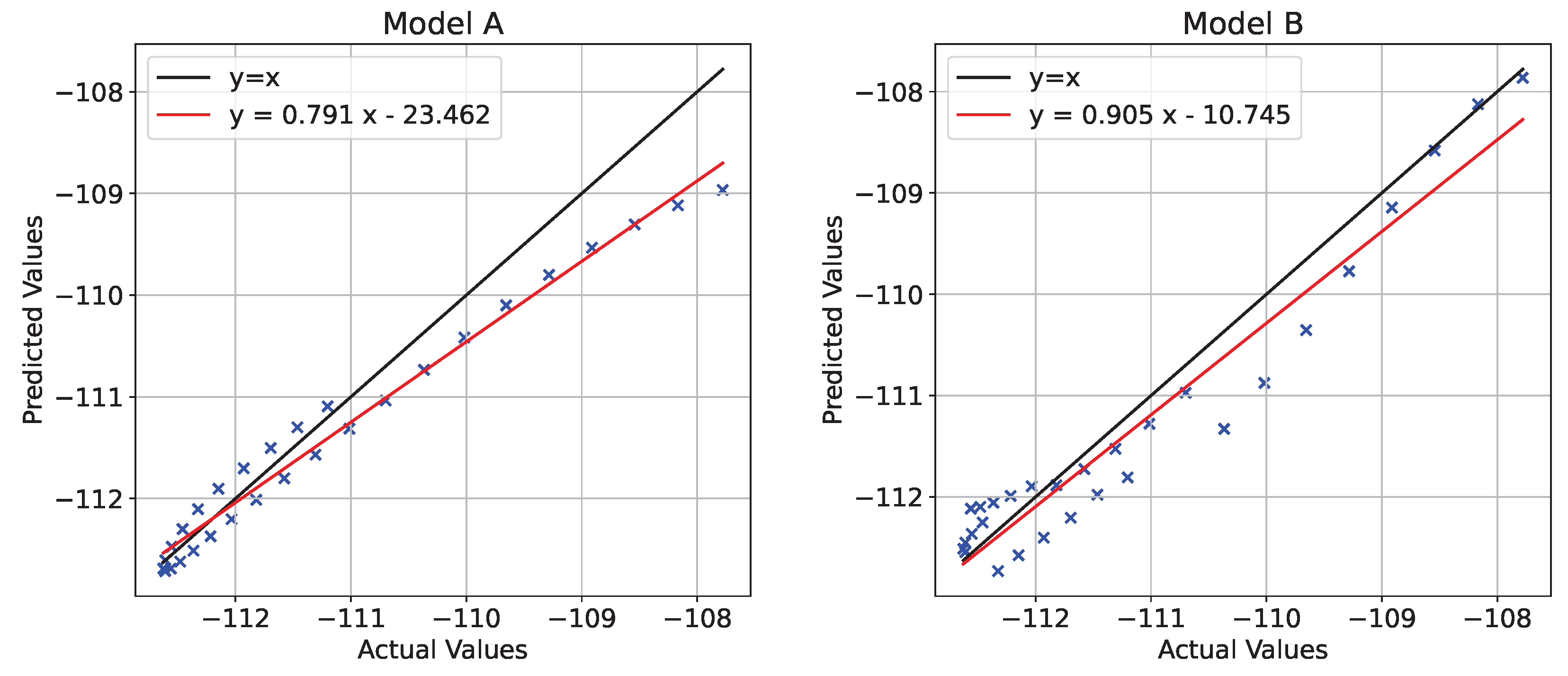
| Linear Baseline | Model A | Model B | |
|---|---|---|---|
| Train MSE | 8.79 | 5.95 ± 0.27 | 5.54 ± 0.46 |
| Test MSE | 7.79 | 6.40 ± 0.11 | 6.03 ± 0.12 |
Disclaimer/Publisher’s Note: The statements, opinions and data contained in all publications are solely those of the individual author(s) and contributor(s) and not of MDPI and/or the editor(s). MDPI and/or the editor(s) disclaim responsibility for any injury to people or property resulting from any ideas, methods, instructions or products referred to in the content. |
© 2023 by the authors. Licensee MDPI, Basel, Switzerland. This article is an open access article distributed under the terms and conditions of the Creative Commons Attribution (CC BY) license (https://creativecommons.org/licenses/by/4.0/).
Share and Cite
Yazbeck, J.; Rundle, J.B. A Fusion of Geothermal and InSAR Data with Machine Learning for Enhanced Deformation Forecasting at the Geysers. Land 2023, 12, 1977. https://doi.org/10.3390/land12111977
Yazbeck J, Rundle JB. A Fusion of Geothermal and InSAR Data with Machine Learning for Enhanced Deformation Forecasting at the Geysers. Land. 2023; 12(11):1977. https://doi.org/10.3390/land12111977
Chicago/Turabian StyleYazbeck, Joe, and John B. Rundle. 2023. "A Fusion of Geothermal and InSAR Data with Machine Learning for Enhanced Deformation Forecasting at the Geysers" Land 12, no. 11: 1977. https://doi.org/10.3390/land12111977