Water Balance Uncertainty of a Hydrologic Model to Lengthy Drought and Storm Events in Managed Forest Catchments, Eastern Australia

Abstract

Interest has grown in applying hydrologic models in managed catchments despite uncertainties around model inputs and empirical relationships to simulate complex geo-hydrological processes of streamflow and sediment variations. Unquantified interactions between geophysical, climate and management indices can also increase simulation uncertainties. Calibration of model outputs against observed values allows identification of the most influential variables and their optimised ranges by which model performance can be enhanced. A rainfall-runoff Soil and Water Assessment Tool (SWAT) model was utilised for four catchments in northern New South Wales, Australia to simulate time series of streamflow across varying rainfall regimes, from dry seasons from 2002 towards rainy 2009. Parameters causing a substantial change on model streamflow outputs were first identified using a sensitivity analysis which indicated that hydrologic factors governing the sources of water supply were critical parameters. These sensitive variables were substantially derived from groundwater modules, basic flow in the main channel, and management practices. Statistical tests of between-catchment differences showed that model simulations performed better in a catchment where the sole rain gauge was installed, while also having the narrowest variations in simulated values (r-index = 0.02). In contrast, the highest uncertainty of model simulations was found in the furthest catchment from the rain gauge where there was not a satisfactory agreement with observed data. Yearly differences between 2002 and 2009 indicated an overestimation of streamflow during low flow periods. However, the calibration process performed well in most peak flows where estimations followed the respective observed values. Long-term dry periods between 2002 and 2007 resulted in an overestimated baseflow by predicting an unrealistic recharge infiltrating aquifers.

1. Introduction

Robust hydrological models are often considered an alternative for the cost and time involved in continuous long-term monitoring of streamflow and water constituents like sediment, bacteria and nutrients. Although hydrologic models can have a capability to simulate long-term changes in water quality of stream networks before applying a particular management practice [1], they need to be tested for reliability by paired comparisons between simulated and observed datasets for a number of gauged streams. Time series simulation of water balance and water quality can also be addressed by hydrological models for ungauged catchments and/or non-monitored years in gauged sites if modelled datasets meet a robust fit with simulations. Despite a heightened interest in the application of such physics-based models, there are still uncertainties about how closely model inputs and empirical relationships have the capability to simulate complex geo-hydrological variations in streamflow and suspended and dissolved load at a catchment scale. Moreover, there are unquantified interactions between geophysical, climate and management parameters affecting the hydrologic status of a catchment [2]. Despite the uncertainties, hydrological models are increasingly being applied to evaluate long-term changes in water quality (e.g., [3,4,5,6]) and annual streamflow following land use changes (e.g., [7]).

The process of model parameterisation often relies on limited information from monitoring and data recording, resulting in increased uncertainty through the use of default values for unquantified variables. The calibration of model outputs against observed values identifies the most influential variables and their optimised ranges by which model performance can be enhanced and validated for a given catchment.

Different hydrologic models with the ability to simulate catchment-wide flow changes following natural and human-induced pressures have been developed. A rainfall-runoff Soil and Water Assessment Tool (SWAT) model [8] was utilised for the study area to simulate the impacts of a varying range of rainfall patterns on streamflow between 2002–2009, the period when flow-monitoring instrumentation had been maintained. Numerous reports indicated a capability of the SWAT model to assess streamflow and water quality changes around the world (e.g., in the USA [9,10]; Switzerland [11]; Republic of Korea [12]; Germany [13]; China [14]; and Australia [15,16,17,18]). The SWAT model was chosen in this study due to its semi-distributed spatial capability to compute within small homogenous units of a subdivided catchment, although model input parameters were considered lumped values regardless of their spatial variability. Furthermore, the model has an ability to perform simulations at daily timesteps [2]. One of the greatest advantages of the SWAT model is post-simulation analyses which enable initially modelled datasets to be matched more closely to observations and with higher accuracy and known sources of uncertainty.

Application of simulated hydrologic models to catchments characterised by sudden and severe fluctuations in the water balance will increase the uncertainty of outputs. Variability in mean annual rainfall in Australia is greater than in comparable regimes elsewhere in the world [19,20], and catchments are often subject to occasional extreme storms and lengthy drought events. Such fluctuations, which may threaten the environmental and economic stability of downstream communities, have been widely reported in the Australian east coast in the last two decades and may also accelerate degradation of aquatic and terrestrial habitats. Vulnerable steep channels in most managed catchments in subtropical northern New South Wales (NSW) are characterised by potentially detrimental soil erosion due to severe rainfall events after lengthy dry periods [21], including in forestry areas here and elsewhere (e.g., [22,23,24,25]. Forestry logging operations and severe hydro-climatic conditions result in domestic water quality in eastern Australian communities often exceeding minimum standards for suspended sediments, nutrients and some herbicides [26].

This study aims to calibrate the SWAT model against observations to identify water balance modules most sensitive to simulation accuracy. Its application will establish how well a physically-based model is capable of efficiently addressing hydrological processes during dry (2002–2007) and wetter seasons (2008–2009), using 8 years of streamflow data and a single rain gauge. Investigation of both spatial and temporal variations in the model’s simulation accuracy will provide a guide to its potential usefulness in managing future land use/land cover and climate-induced high flows.

2. Materials and Methods

The SWAT model will be applied to information and data relating to the study area. An outline of the study area will be followed by:

• A brief summary of the SWAT model
• Model requirements as related to the study area (spatial inputs, temporal inputs)
• Procedures for model calibration and evaluation
• Initial sensitivity analysis of model variables using study area streamflow data

2.1. Study Area

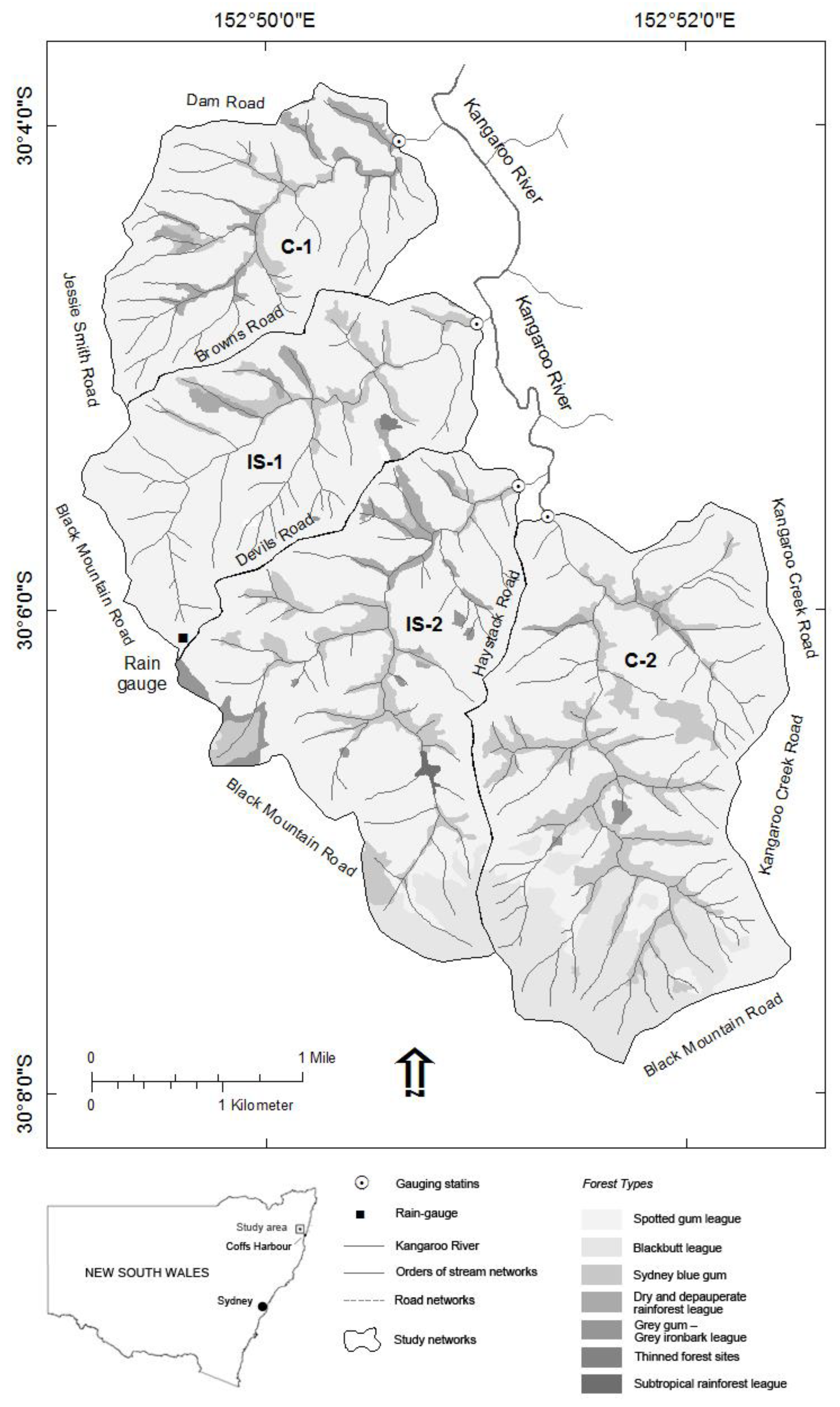
The study was carried out in four neighbouring managed catchments of native eucalyptus forest in the Kangaroo River State Forest in northern NSW, Australia (Figure 1). The catchments with a total of 2173 ha (approx. 21 km²) consisted of two non-harvested control (C-1 and C-2) catchments and two selectively harvested (single-tree) impact catchments (IS-1 and IS-2) where rainfall and streamflow were measured between 2002 and 2009 by the forestry authorities.

The topography involves a range of gradients with steep mountainous slopes and mainly V-shaped valleys to moderately sloping natural terraces. The study area generally has a north-eastern aspect and elevation ranges from 160 m above sea level at the most downstream point to 560 m at the highest ridgetop. The region generally has a subtropical climate that is moderated by the maritime influence of the Pacific air mass [28]. Geology is dominated by Carboniferous Coramba beds comprising lithofeldspathic wacke, minor siltstone, siliceous siltstone, mudstone, metabasalt, chert and jasper, with rare calcareous siltstone and felsic volcanics [29,30]. Soils are mostly shallow and are mixed with roots and gravel particularly on steep hillslopes adjacent to streams. Soil landscapes in the study area are generally Black Mountain with lesser areas of deep (>150 cm) well-drained Yellow Earths formed on siltstones. The Black Mountain soil type consists of loamy and occasionally silty textures in the A horizon together with clay loam and commonly silty textures in the B horizon. Moderately deep to deep (>100 cm) well-drained Yellow Earths and Brown Earths occur on other lithologies [31]. The dominant vegetation type is a mixed species of native evergreen Eucalyptus forest occupied by a dense layer of understorey [30]. This forest type covers most of the area and includes five main species (Corymbia maculata, Eucalyptus saligna, E. pilularis, E. grandis, and E. paniculata) with the addition of minor species along drainage lines. In the current study, the impacts of single-tree logging operations (carried out over a few months in parts of IS-1 and IS-2) were disregarded.

2.2. A summary Description of the SWAT Model

The Soil and Water Assessment Tool (SWAT) is a physically-based hydrologic model simulating time series of water quantity and quality at a catchment outlet, developed by the US Department of Agriculture, Agriculture Research Service (USDA-ARS). The SWAT is a semi-distributed model where a given value is assigned to each hydrologic response unit (HRU) using spatially distributed lumped values within each subdivided sub-catchment. The HRUs are fundamental computational units upon which model simulations are performed. The simulated streamflow values at the HRU scale are aggregated for a sub-catchment and then for a catchment.

The hydrologic simulation is based on water balance equations and thus incorporates interception, evapotranspiration, surface runoff, infiltration, soil percolation, lateral flow, groundwater flow and channel routing processes [13]. The hydrologic component of SWAT uses the Natural Resources Conservation Service (NRCS) runoff curve-number (CN) equation [32]. Surface runoff from daily rainfall was estimated using a modified SCS curve number method, which relates the potential of runoff to land cover, soil properties, and antecedent moisture condition. Groundwater flow contribution to total streamflow is simulated by routing a shallow aquifer storage component to the streams. The water balance for the shallow aquifer considers the recharge stored in the shallow and deep aquifers and groundwater baseflow into rivers. Recharge is defined by the amount of surface water entering the aquifer, the total amount of water exiting the bottom of the soil profile and the delay time produced by the overlying geologic formations (GW_DELAY). A fraction of the total daily recharge can be routed to the deep aquifer. The amount of water moving from the shallow aquifer due to percolation into the deep aquifer is correlated to the aquifer percolation coefficient (RCHRG_DP) and the amount of recharge entering both shallow and deep aquifers [33]. The deep aquifer contributes baseflow to the main channel or reach within a sub-catchment. Baseflow is allowed to enter the river only if the amount of water stored in the deep aquifer exceeds a threshold value specified by the user, GWQMN [13]. A detailed description of the SWAT model and its simulation processes have been described in previous reports (e.g., [34,35,36,37]).

2.3. Model Input Data Requirements (Parameterisation)

In this study, the SWAT model was executed using an extension of ArcSWAT version 2012.10.1 [34] within ArcMap 10.0 [38] to incorporate spatially distributed data. Spatial inputs to the model consisted of raster layers of a digital elevation model (DEM), soil landscape, and land use/land cover along with geographic positions of streamflow gauging stations (

Table 1. Data and sources for catchment characteristics.

Data	Resolution and Lab Analysis	Source
Streamflow	Sub-daily, averaged to daily, 2002–2009	Forestry Corporation of NSW
Rainfall	Daily, 2002–2009	Forestry Corporation of NSW
Temperature	Daily, 2002–2009	Bureau of Meteorology, NSW; Dorrigo station 059140
DEM—Slope steepness	10 × 10 m SPOT 5 imagery (2011)	Department of Primary Industries, NSW
Land use	10 × 10 m SPOT 5 imagery (2011)	Department of Primary Industries, NSW
Land cover	10 × 10 m SPOT 5 imagery (2011)	Department of Primary Industries, NSW and field observations
Soils	1:100,000 map [31] and field sampling (n = 41) at grid intersections 500 × 1000 m; lab analysis	Milford [31] and field sampling/lab analysis (n = 41)

; Figure 1 and Figure 2). A 10-m by 10-m spatial resolution DEM was used to define geographic features for the model such as catchment boundaries and stream networks (Figure 1; Table 1). Temporal variables included time series of daily rainfall and air temperature as well as sub-daily streamflow records.

2.3.1. Spatial Inputs

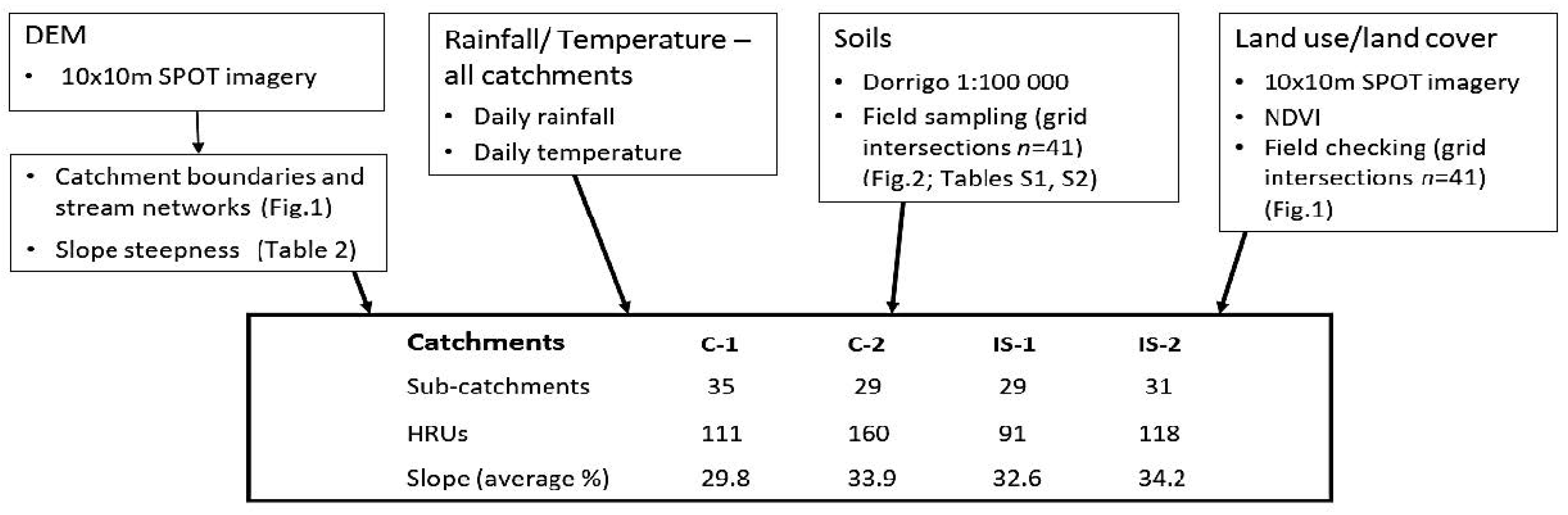
Of the spatial parameters, slope steepness of the catchments was classified into three groups for areas having <35, 35–45 and >45% by which varying topographic heterogeneity were equally included within each category. Of the four catchments, C-1 had the lowest mean slope length, gradient and steepness; and IS-2 had the highest mean slope length, gradient and steepness (p < 0.05) [21] (

Table 2. Catchments, sub-catchments, HRUs and slopes.

Catchment	C-1	C-2	IS-1	IS-2
Sub-catchments (no.)	35	29	29	31
Grid cells (no.)	36,735	65,535	44,293	59,278
HRUs (no.)	111	160	91	118
Average slope (%) *	29.8 d	33.9 b	32.6 c	34.2 a
Standard error (%)	0.063	0.063	0.060	0.062
Coefficient of variation	0.403	0.479	0.387	0.439
Maximum slope (%)	74.7	97.3	77.0	92.3

* Different letters represent statistical significance (p < 0.05) using the Kruskal-Wallis test. Letters a to d indicate the order of values from maximum to minimum.

).

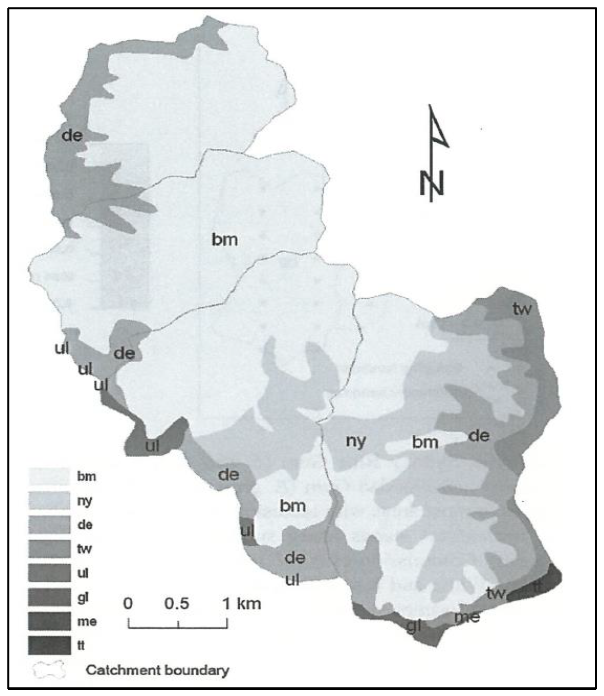
Soil series were obtained from Soil Landscapes of the Dorrigo 1:100,000 map sheet [31]. Soil types were classified into eight categories across the four catchments (Figure 2 and Figure 3). Details of each layer of a given soil type were considered for calibration of the model (see [31]): soil texture, available water content, hydraulic conductivity, bulk density, and organic carbon content. Hydrologic and physical properties of soil types in the study area are presented in Tables S1 and S2 and these data form the basis on which soil variables were parameterised in the SWAT model. One of the key attributes of the model is “hydrologic soil group” which was determined using a definition by the USDA Natural Resources Conservation Service [39] as a function of hydraulic conductivity of soil layers.

Land use/land cover raster data layers were generated by interpretation of 10-m resolution SPOT satellite imagery of 2011 (the closest date to the 2002–2009 streamflow recording period) followed by field surveys. The dominant land use in the catchments consisted of an evergreen forest (FRSE code in the model); seasonal and annual changes in land cover values over the study period and to 2011 were minimal. Evergreen forest occupied as much as 93.4, 92.7, 94.1 and 93.8% of the total area of C-1, C-2, IS-1 and IS-2, respectively for each study year. Approximately 6.4, 5.9, 5.4 and 5.5%, respectively, of these catchments included water bodies (WATR) predominantly featured as stream networks. The remaining land uses, ranging between only 0.2 and 1.4% of the study area, were gravel roads, skid trails and log depots and were all classified as urban areas (URBN).

Sub-catchments are further sub-divided into HRUs based on adjusting a threshold area of soil, land use and slope. These data layers were overlayed in ArcMap to define small-scale homogeneous HRUs. A sub-catchment was defined by the model based on stream junctions and similarities in soil, land use and slope features. As a basis for computations, areas of land use and soil greater than the threshold area of 10% of a sub-catchment were bounded as a unique HRU. The study area was delineated into 111, 160, 91 and 118 HRUs from 35, 29, 29 and 31 sub-catchments in C-1, C-2, IS-1 and IS-2, respectively (Table 2).

2.3.2. Temporal Inputs

Temporal data included continuous daily weather records (2002–2009) which were obtained from stations installed inside and near the catchments by Forestry Corporation of NSW (formerly known as Forests NSW) and the Australian Bureau of Meteorology. A single rain gauge installed by the Forestry Corporation was used in the study area because other gauges were damaged after severe storms. The rainfall data monitored in IS-1 was the only continuous record over the period 2002 to 2009, and this was therefore also used for the adjacent catchments; rainfall distribution was assumed to be constant across a catchment. Daily minimum and maximum temperatures were records from Dorrigo meteorological station (No. 059140) [41,42] which is about 30 km south of the rain gauge (centroid of the study area).

A streamflow gauging station was installed by the Forestry Corporation of NSW at the outlet of each study catchment to continuously record sub-daily values between 2002 and 2009, after which the Corporation’s recording program ceased. Because the SWAT model is unable to simulate streamflow in subdaily timesteps, data were averaged to daily values. The geographic positions of the streamflow gauging stations, along with rainfall and temperature records, were used for HRU-based simulations for each catchment. Daily streamflow data from the four gauging stations were used for calibration and validation. A warm-up period is required to set model inputs and empirical equations to determine initial statuses for storage volumes [43]; daily data for 2002 were used for this period. Since annual rainfall had been consistently rising from 2002 towards 2009 in the region, a six-year (January 2003 to December 2008) record of daily streamflow was used for calibration of the model to cover a wide range of dry and wet weather conditions. The 2009 dataset was used for validating calibrated parameters in the model.

2.4. Model Calibration and Evaluation

Hydrologic calibration of the model consisted of adjusting process-related model parameter values within reasonable ranges, with an emphasis on water balance variables in the current study, to modify numerical variability between simulated and observed streamflows individually for each of the catchments [25,44,45]. The model calibration consisted of providing sufficient required measured inputs as well as the relative significance of all variables involved in the model, whether measured or estimated, for a satisfactory agreement between simulated and observed values.

Calibration evaluation involved establishing how closely modelled data matched observations. Visual comparisons and quantitative statistics were performed between the observed and simulated values to assess the uncertainty of modelling, using the coefficient of determination (R²), the Nash-Sutcliffe Efficiency (NSE) and the mean squared error (MSE). Model performance was also evaluated by percent bias (PBIAS) [1]. Both NSE and R² are considered to be particularly sensitive to peak flow conditions [46]. Details of the correlation and error tests can be found in [1,35,47].

A satisfactory fit coefficient to evaluate the efficiency of SWAT outputs varies depending on the number of study years, the purpose of simulations, user-required precision, quality and amount of gauged recording, and hydro-geomorphic conditions of catchments. A minimum satisfactory coefficient of modelled outputs was considered following the results of [1,35]. Hence, the model simulation for streamflow was evaluated as being indicative of a satisfactory fit if NSE > 0.5, R² > 0.5 and PBIAS ±25%. If the statistical indices did not meet the required criteria for an efficient simulation, the calibration process of the model was repeated followed by further evaluation of statistical tests. The NSE was determined as a statistical target in this study upon which a significantly best simulation was chosen. A total number of 14–15 SWAT input parameters were selected for model calibration, with most of these relating to channel and landscape characteristics. As many as 1000 simulation runs were performed for each repetition. A total of 20,000–30,000 model runs were conducted for each catchment to examine the significance of each sensitive parameter in obtaining an efficient simulation output.

2.5. Sensitivity Analysis

Key parameters causing a significant change in model outputs were first identified using a sensitivity analysis [1]. Sensitive variables were detected following the first calibration run involving 1000 simulations if a change in a variable caused a significant difference between observations and simulations with p-value < 0.05 and t-statistic > 2.0. It was found during early calibration iterations that the modelled values were highly significant to water balance-related modules. Therefore, adequate groundwater and channel sediment delivery parameters were included in the calibration process to produce more accurate calibration adjustments (

Table 3. A list of the variables used in the sensitivity analysis and their initial default values.

Parameters	SWAT Extension File	Description (Unit) 1	Initial Value
ALPHA_BF	.gw 2	Baseflow recession constant (days)	0.048
GW_DELAY	.gw	Groundwater delay time (days)	31
REVAPMN	.gw	Threshold depth for water in the shallow aquifer for percolation to the deep aquifer to occur (mm)	1.0
GWQMN	.gw	Threshold depth of water in the shallow aquifer for return flow to occur (mm)	0.0
RCHRG_DP	.gw	Deep aquifer percolation factor (fraction)	0.05
GW_SPYLD	.gw	Specific yield of the shallow aquifer (m3/m3)	0.003
GW_REVAP	.gw	Represents water movement from the shallow aquifer to the root zone (unitless)	0.02
GWHT	.gw	Initial groundwater height (m)	1.0
PHU_PLT	.mgt 3	Total number of heat unit	0.0
CN2	.mgt	Initial SCS runoff curve number (unitless)	55–77
TDRAIN_BSN	.bsn 4	Time to drain soil to field capacity (hours)	0.0
DDRAIN_BSN	.bsn	Depth to sub-surface drain (mm)	0.0
SURLAG	.bsn	Surface runoff lag coefficient (unitless)	4.0
EVRCH	.bsn	Reach evaporation adjustment factor (unitless)	1.0
SPEXP	.bsn	Exponent parameter for calculating sediment reentrained in channel sediment routing (unitless)	1.0
EROS_SPL	.bsn	The splash erosion coefficient (unitless)	1.5
SOL_AWC	.sol 5	Available water capacity of the soil layer (mm H2O/mm soil)	See Tables S1 and S2
SOL_K	.sol	Saturated hydraulic conductivity (mm/hr)
SOL_ALB	.sol	Moist soil albedo (unitless)
SOL_CRK	.sol	Potential or maximum Crack volume of a soil profile (unitless)	0.5
CH_K2	.rte 6	Effective hydraulic conductivity in main channel alluvium (mm/hour)	0.0
CH_N2	.rte	Manning’s “n” value for the main channel (unitless)	0.014
EPCO	.hru 7	Plant uptake compensation factor (unitless)	1.0

¹ [8]; ² groundwater; ³ management; ⁴ basin; ⁵ soil; ⁶ routing; ⁷ HRU.

).

Uncertainty and sensitivity analyses of the SWAT model outputs were conducted using the Sequential Uncertainty Fitting Version 2 (SUFI-2) algorithm [10]. The SUFI-2 is one of the algorithms interfaced in the SWAT Calibration and Uncertainty Programs (SWAT-CUP) package. SWAT-CUP was manually linked to the output TextInOut directory generated by the SWAT model. The sensitivity analysis implemented in the SUFI-2 algorithm includes an automatic procedure based on Latin-Hypercube (LH) simulations and One-factor-At-a-Time (OAT) sampling procedure [48]. The LH-OAT approach consists of a range of input parameters and identifies the role of one parameter on numerical changes in model outputs while other variables are held constant. The uncertainty of model outputs was measured by the 95% prediction uncertainty (95PPU) in the SUFI-2 algorithm. The p-index is calculated at the 2.5% and 97.5% limits of the cumulative distribution of output variables and is expressed as a percentage of measured data covered within the estimated 95PPU limit. The r-index is another uncertainty measure that determines an average thickness of a 95PPU band divided by the standard deviation of the measured data. The latter coefficient of uncertainty of the model simulations is calculated as follows [11,43,45,49]:

$$r–index=[\frac{1}{n}{\displaystyle \sum }_{i=1}^n\left(Y_{97.5\%}-Y_{2.5\%}\right)]/{\sigma }^{obs}$$

where Y_97.5% and Y_2.5% represent the upper and lower limits of the 95PPU for a modelled variable, and $\mathsf{\sigma }$^obs is the standard deviation of the measured data. A perfect index of 1 (100%) for the p-index and 0 for the r-index indicates the strength of simulation certainty compared to observations. More detail is presented by previous studies such as [11] and [50]. Once optimised input parameters were determined within the permissible range of input parameters during the sensitivity and calibration (2003–2008) stages, observed daily streamflows for the 2009 datasets were applied for validation of the calibrated variables to confirm the certainty of modelling results.

3. Results and Discussion

3.1. Calibrating Sensitivity Parameters

In this study, modelled values were first calibrated against observations to prioritise the significance of sensitive parameters. Land use was temporally and spatially uniform throughout the catchments, unlike variations reported in some other studies (e.g., [51]), so the land use variable was removed from further consideration.

Table 4. Summary of calibrated values for the sensitively ranked parameters for each study catchment.

	Catchment C-1					Catchment C-2
Sensitivity Ranks	Replacement Method	Parameters (Extension File)	New Range			Replacement Method	Parameters (Extension File)	New Range
1	v 1	ALPHA_BF (gw) 2	0.034	0.064		v	ALPHA_BF (gw)	0.008	0.012
2	v	CH_K2 (rte)	286.391	349.431		v	CH_N2 (rte)	−0.242	−0.226
3	v	CH_N2 (rte)	−0.029	−0.016		r	CN2 (mgt)	0.025	0.030
4	r 3	CN2 (mgt)	0.004	0.016		v	CH_K2 (rte)	252.231	296.357
5	v	TDRAIN_BSN (bsn)	25.841	35.873		v	SURLAG (bsn)	14.830	15.781
6	v	DDRAIN_BSN (bsn)	436.066	529.784		v	TDRAIN_BSN (bsn)	18.038	21.593
7	r 3	SOL_AWC (sol)	−0.037	0.066		v	RCHRG_DP (gw)	0.977	0.982
8	v	GW_DELAY (gw)	6.758	46.348		v	GWQMN (gw)	4346.397	4476.475
9	r	SOL_K (sol)	−0.415	−0.306		r	GW_SPYLD (gw)	0.497	0.524
10	v	REVAPMN (gw)	977.404	1031.533		r	SOL_K (sol)	−0.413	−0.402
11	r	SOL_ALB (sol)	0.056	0.081		r	EVRCH (bsn)	−0.062	−0.055
12	v	GWQMN (gw)	1773.300	2088.247		r	SOL_AWC (sol)	0.339	0.359
13	v	SURLAG (bsn)	0.535	0.833		v	GW_DELAY (gw)	371.910	385.371
14	v	RCHRG_DP (gw)	0.385	0.394		r	SOL_ALB (sol)	0.142	0.159
15	r	GW_SPYLD (gw)	0.010	0.074		v	GW_REVAP (gw)	0.105	0.107
	Catchment IS-1					Catchment IS-2
1	v	CH_K2 (rte)	156.761	163.736		v	ALPHA_BF (gw)	0.055	0.075
2	v	ALPHA_BF (gw)	0.988	0.995		v	CH_K2 (rte)	175.302	206.273
3	v	CH_N2 (rte)	0.335	0.354		v	CH_N2 (rte)	−0.023	0.096
4	r	CN2 (mgt)	0.072	0.094		r	CN2 (mgt)	−0.432	−0.426
5	v	SURLAG (bsn)	3.303	3.871		r	SOL_K (sol)	−0.980	−0.815
6	r	SOL_AWC (sol)	−0.052	−0.010		v	SURLAG (bsn)	3.807	4.237
7	r	SPEXP (bsn)	0.168	0.221		r	SOL_AWC (sol)	−0.007	−0.001
8	v	RCHRG_DP (gw)	0.242	0.275		v	REVAPMN (gw)	261.284	321.025
9	v	GW_REVAP (gw)	0.104	0.109		v	PHU_PLT (mgt)	2308.944	2714.646
10	v	GWHT.gw	8.374	12.759		v	GW_DELAY (gw)	387.711	455.068
11	r	SOL_CRK (sol)	0.008	0.029		v	RCHRG_DP (gw)	0.348	0.392
12	r	EPCO (hru)	0.028	0.039		v	GWQMN (gw)	2244.404	3032.098
13	v	GWQMN (gw)	1816.665	2487.552		r	EROS_SPL (bsn)	0.062	0.042
14	v	GW_DELAY (gw)	20.758	68.068		v	GWHT (gw)	1.901	2.974

¹ Substitution of a parameter’s value by new calibrated ranges ² Bold parameters are significantly (p < 0.05) sensitive following the first calibration iteration ³ Initial parameter values were multiplied by (1+ relative “r” value).

summarises major and minor influential parameters following sensitivity analysis of streamflow for each of the catchments.

The calibration and sensitivity analyses (Table 4) showed that some parameters had a significantly (p < 0.05) greater impact than others on simulated streamflow outputs. The baseflow recession ALPHA_BF factor used in the SWAT groundwater (.gw) file had the greatest significance in three catchments (C-1, C-2, IS-2) and was the second most important parameter in IS-1 (Table 4). The baseflow recession constant is a direct index of groundwater flow in response to changes in recharge [13]. In addition, the time series of simulated streamflow was subsequently sensitive to main channel characteristics affecting the potential of sediment delivery. The effective hydraulic conductivity (CH_K2) and the Manning’s “n” roughness coefficient (CH_N2) for main channels also had significant effects on the modelled streamflow values, followed by the management SCS curve number for antecedent moisture condition (CN2). Similar significant sediment routing factors were reported by [52].

3.2. Sensitivity of Key Parameters

With sensitivity significance (p-value) of 0.020, 0.027, 0.000 and 0.002, streamflow fluctuations were influenced by geomorphologic processes involving the time taken to drain soil to field capacity (TDRAIN) in C-1 and the surface runoff lag coefficient (SURLAG) in C-2 and IS-1, as well as the available water content of soil (SOL_AWC) in IS-1 (Table 4). In general, sensitivity analysis indicated that hydrologic factors governing the sources of water supply were critical parameters influencing streamflow outputs. A set of the model-sensitive parameters was achieved from groundwater conditions (.gw), flow of water and sediment in the main channel (.rte) and management practices (.mgt). Model simulations were not significantly sensitive to other selected variables. Water flow in the study area was thus predominantly influenced by saturation and the interaction between groundwater and surface water.

3.2.1. Baseflow Variability

The simplicity of the SWAT model in simulating baseflow variability was particularly critical in the subtropical environment of the study area where lengthy dry conditions in winter months (southern hemisphere) are followed by episodic storm events in the spring and mostly summer months when the amount of recharge entering and being stored in an aquifer increases. Storm events create lagged baseflow from deep aquifers, producing unexpectedly great streamflow particularly during low rainfall periods. Conversely, the recharge of water flowing to deeper aquifers as a result of storm events following long-term dry conditions may generate a low streamflow along high-infiltrating runoff paths and channels before reaching an outlet. Constant wet days may subsequently result in an unexpected increase in baseflow later, therefore triggering a higher flow of water than simulated under a given rainfall amount.

Some work has been conducted to shift the SWAT model of infiltration-excess runoff towards a saturation-excess-based runoff by redefining HRUs [53]. The water balance-based SWAT performed more efficiently in simulating spatial runoff dynamics and saturation-excess areas to calculate runoff volumes [54,55]. These researchers [54,55] used a soil wetness index SWAT to address saturation excess as the dominant runoff process in the Himalayan landscape. A case study in lowland catchments in Northern Germany [13] also found that simulated streamflow was mainly sensitive to groundwater and soil indicators. The most influential parameter was identified as the threshold water level in a shallow aquifer for baseflow (GWQMN), followed by other groundwater-related factors RCHRG_DP, ALPHA_BF, GW_REVAP and GW_DELAY [13]. In another study in Tanzania, sensitivity analysis was carried out in a catchment covering an area of 7280 km² and results showed that CN2, RCHRG_DP, SLOPE and SOL_Z had the greatest significance in the SWAT model [56].

Some researchers have recommended that application of SWAT coupled with a groundwater module (gwflow) will provide more realistic insights for an accurate representation of groundwater processes and their interaction with surface water [57,58]. Investigation of the dynamics of groundwater flow and its multiple interactions with catchment characteristics at different spatial and temporal scales has highlighted the complexities involved in modelling baseflow during drought periods [59]. Our study area was directly (.gw and .rte parameters) or indirectly (.mgt parameters) vulnerable to water balance indicators. Empirically estimated as a function of soil permeability, land use and hydrologic condition, the CN curve number factor is a proportion of rainfall excess that appears as either runoff flow or water retention in soil. The SWAT model efficiency has been improved by revisiting the CN factor using terrace slope, precipitation intensity and soil moisture [60]. Several researchers have reported that simple groundwater modules in the SWAT model limit its ability to efficiently simulate water balance cycles in a catchment (e.g., [16,52,61]).

3.2.2. Site-Specific Parameter Optimization

The sensitivity algorithms did not conform to a particular formula in adjusting the SWAT parameters. In order to apply optimised ranges of a given parameter for ungauged adjacent catchments, the variables require a consistent change in response to calibration under similar conditions. A lack of similar decrease or increase in an optimised variable during the sensitivity analysis in this study indicates that any change in a variable during calibration is site-specific and parameters should be separately adjusted for each catchment. For instance, the baseflow recession (ALPHA_BF) factor reduced between 0.008 and 0.012 days (83–75% decrease) in the largest catchment C-2 while it increased about twenty times, ranging between 0.988 and 0.995 days, in IS-1 (Table 4). The dissimilarity of changes in variables under similar site conditions raises concern over the model’s potentially unrealistic mechanism of adjusting simulations during the calibration step and whether new values logically represent catchment conditions.

Between-catchment comparisons of the statistical diagnostics showed that model simulations performed better in IS-1 relative to other sites: IS-1 had the lowest uncertainty in simulating hydrologic processes during the calibration period. This result may relate to the presence of the sole rain gauge installed on the hilltop of IS-1. A relatively satisfactory fit was obtained for the adjacent northern catchment C-1, with a poorer fit being generated for C-2 and IS-2, suggesting that distance to a rainfall recording station assists in achieving an efficient and representative simulation (

Table 5. Statistical results of fitness between observed and simulated values.

Catchments	NSE			MSE			R2			PBIAS
	Simul.1 1 (2003–2008)	Calib 2 (2003–2008)	Validated (2009)	Simul.1 (2003–2008)	Calib. (2003–2008)	Validated (2009)	Simul.1 (2003–2008)	Calib. (2003–2008)	Validated (2009)	Simul.1 (2003–2008)	Calib. (2003–2008)	Validated (2009)
C-1	−5.89	0.26	0.31	0.0239	0.0026	0.0150	0.27	0.43	0.47	−6.07	−2.34	−1.03
C-2	−13.88	0.35	−0.69	0.1995	0.0092	0.1305	0.33	0.36	0.21	−3.97	0.19	0.48
IS-1	−0.19	0.41	0.30	0.0201	0.0099	0.0940	0.37	0.44	0.48	−2.90	−0.77	0.34
IS-2	−31.23	0.01	−7.33	0.0639	0.0020	0.1009	0.38	0.50	0.26	−12.76	−3.24	−1.12

¹ Simul.1 is initially simulated ² Calib. is calibration.

). In addition, instantaneous weather input data are spatially variable across the small catchment-wide area and a gradient of interpolated raster layers from several rain gauges could enhance model performance. Investigators who evaluated the effects of geographic location and frequency of rainfall stations on SWAT streamflow simulations found a substantial negative impact when rainfall and streamflow gauging stations were spatially distanced and recommended that a minimum of four rain gauges are required to obtain accurate streamflow simulations [62]. This figure may vary depending on catchment sizes and topographical differences.

3.3. The Calibration Period

The calibration period (2003–2008) produced a relatively satisfactory agreement between observed daily streamflow and initially-simulated streamflow (Table 5). The NSE coefficients were 0.26, 0.35, 0.41, and 0.01 for the best calibration iteration at gauges in C-1, C-2, IS-1 and IS-2, respectively (Table 5). These coefficients show marked improvements on the initial SWAT simulations for each catchment. In addition, error residuals of the calibrated time series were much lower than the initial simulations so that the MSE was reduced largely by calibration of the initial datasets. The PBIAS values varied from −12.76 to −2.90 for the initial simulations and ranged between −3.24 and 0.19 during calibration. Although the calibration procedure provided higher correlation and lower error bias, the degree of adjustment to achieve higher certainty of simulations differed from one catchment to another.

3.4. Temporal Differences in Statistical Diagnostics

In the current study, low correlations between observations and simulations of daily timesteps improved when data were combined into monthly and annual averages (

Table 6. Correlations (R², NSE) between simulated and observed streamflows over daily, monthly and annual timesteps.

Timestep	Correlation	Catchment C-1	Catchment C-2	Catchment IS-1	Catchment IS-2
Daily	R2	0.43	0.36	0.44	0.50
	NSE	0.26	0.35	0.41	0.01
Monthly	R2	0.58	0.39	0.58	0.48
	NSE	0.58	0.36	0.57	0.40
Annual	R2	0.90	0.74	0.91	0.72
	NSE	0.72	0.73	0.60	0.30

). The low NSE values for daily simulations, compared with monthly and annual timesteps, are in agreement with previous literature. For example, a part-catchment study of 26,400 km² in Texas reported daily NSE was 0.72 between observed and simulated streamflow values from 1995 to 2010 [63]; coarser temporal resolutions had greater NSE coefficients of 0.85 and 0.90 for monthly and annual timesteps, respectively [63]. The SWAT model was also applied to an area of approximately 360 km² in the same catchment, with an NSE as low as 0.05 for daily data, improving to 0.50 for monthly datasets [64]. In a basin in northeastern Europe, model performance was better for monthly than daily flow data (NSE of 0.83 compared with 0.66) [65]; and SWAT performed well when using calibrated monthly timesteps in a Himalayan catchment [66].

Following validation of the calibrated hydrologic input parameters, SWAT output accuracy decreased slightly in the study area during the validation period (2009), except for C-1 (details in Table 5). Model simulation presented a fairly satisfactory agreement with the observed streamflow data in IS-1 (NSE of 0.30, PBIAS of 0.34). Negative PBIAS values of initially simulated streamflow in C-1 and IS-2 indicate a model overestimating bias while C-2 showed underestimating bias during the calibration period. Catchments C-2 and IS-1 underestimated streamflow during validation (Table 5).

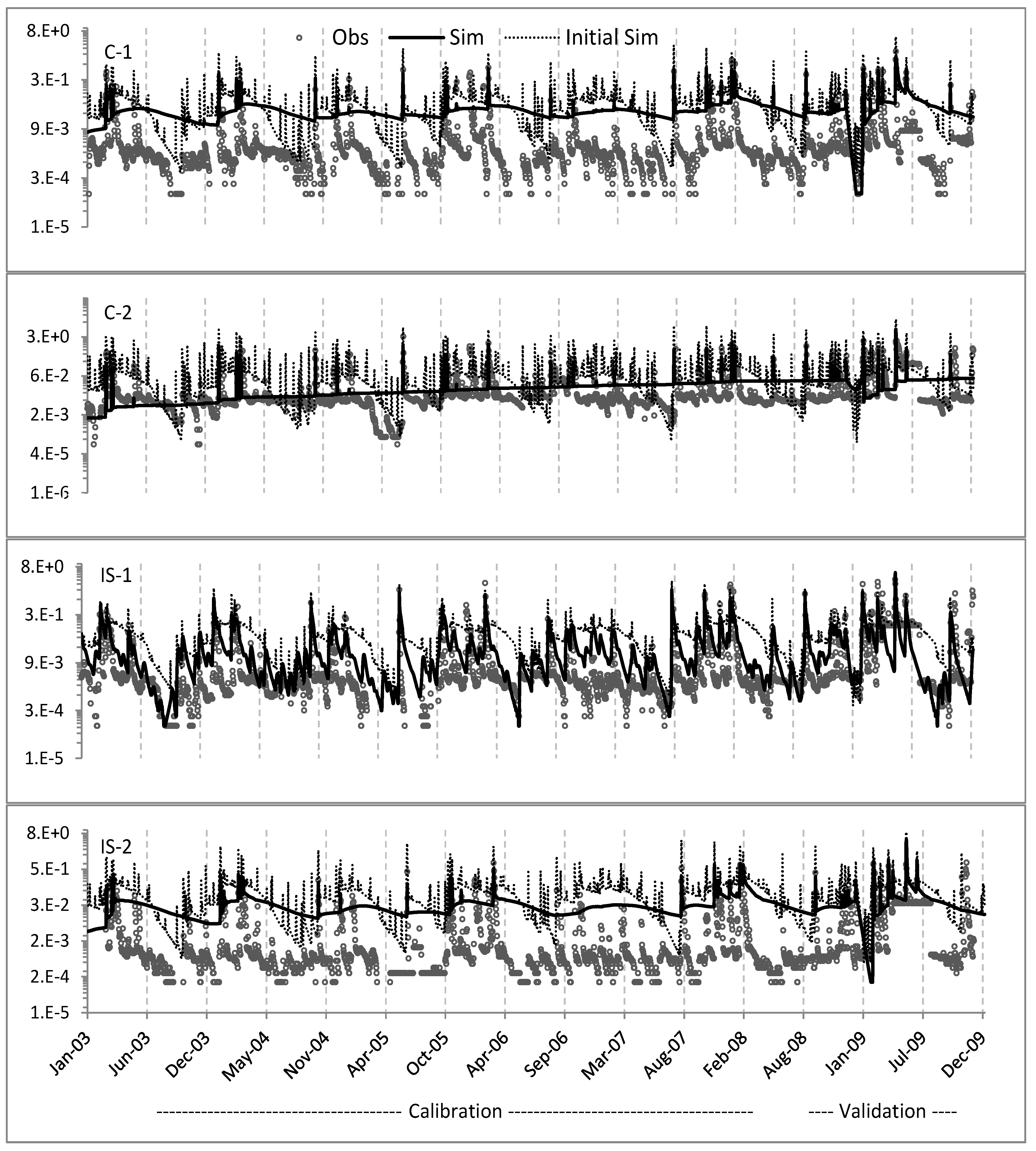
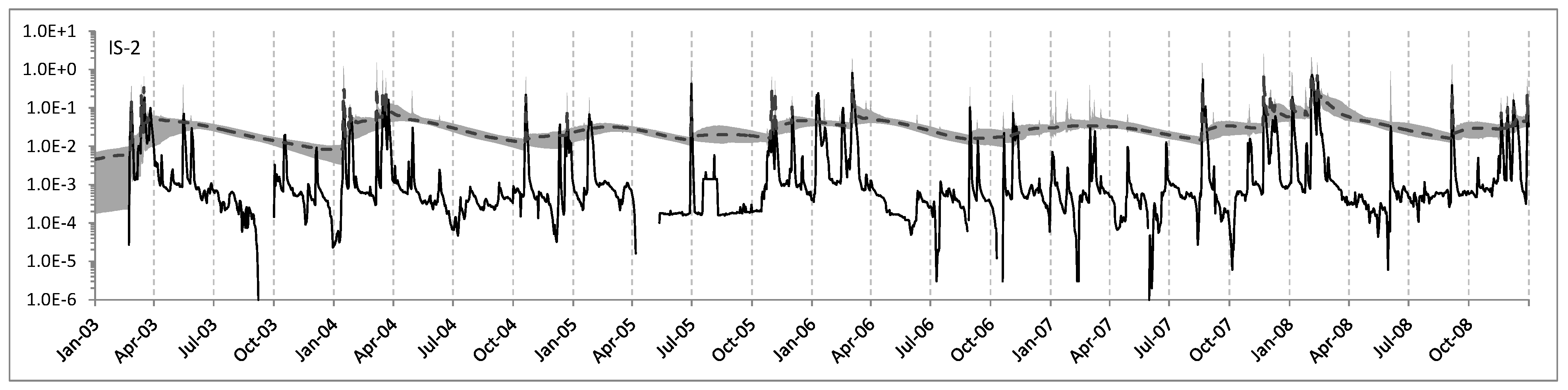
Visual assessment of the observed daily records (2003–2009) against initially simulated and calibrated hydrographs for the periods of calibration (2003–2008) and validation (2009) is presented in Figure 4 for each catchment outlet. Overestimation of initially simulated hydrographs was optimised by repeated calibrations, although the calibrated model still overestimated daily streamflow in all four catchments. The dynamics (rising and falling limbs) of the simulated hydrograph did not overlay properly with the observations in C-1, IS-2 and particularly with the furthest catchment from the rain gauge, C-2. However, the modelling of streamflow in IS-1 produced good results not only for low flows but also during peak streamflows. The single rain gauge was located on hilltops of IS-1 and a great deal of uncertainty was apparent for sites located further from the rain gauge. Authors [63] also noted that lack of a gradient resulting from the use of interpolated rainfall distributions, rather than data recorded from several gauges, may add to model uncertainty.

3.5. Wet/Dry Periods and Simulated Values

Figure 4 shows the overestimations of streamflow during low flow periods of the study years, whereas the calibration process performed well in most periods of peak flows when estimations fluctuated similarly with the respective observed values. This satisfactory calibration was most apparent for IS-2. A possible explanation of the overestimated baseflows may be provided by the long-term dry period (2002–2007) during which the simulations of water balance were unrealistic for low flow hydrological cycles. During dry and/or low flow seasons, aquifer recharge probably exceeded the proportion of interflow emerging as baseflow, resulting in overestimation of streamflow [16]. In a study in southeastern Victoria, Australia, SWAT was applied to a 1200-km² catchment for modelling monthly streamflow [16]. These results showed that the groundwater variables did not perform properly and were greatly simplified, thus providing a poor representation of baseflow conditions. The SWAT model was also applied to a 300-km² catchment in central Queensland, Australia to predict the impact of agricultural management on sediment load, resulting in an overestimated total flow [15]. Despite major differences in catchment areas, overestimates attributed to unreliable groundwater estimations appeared in each study.

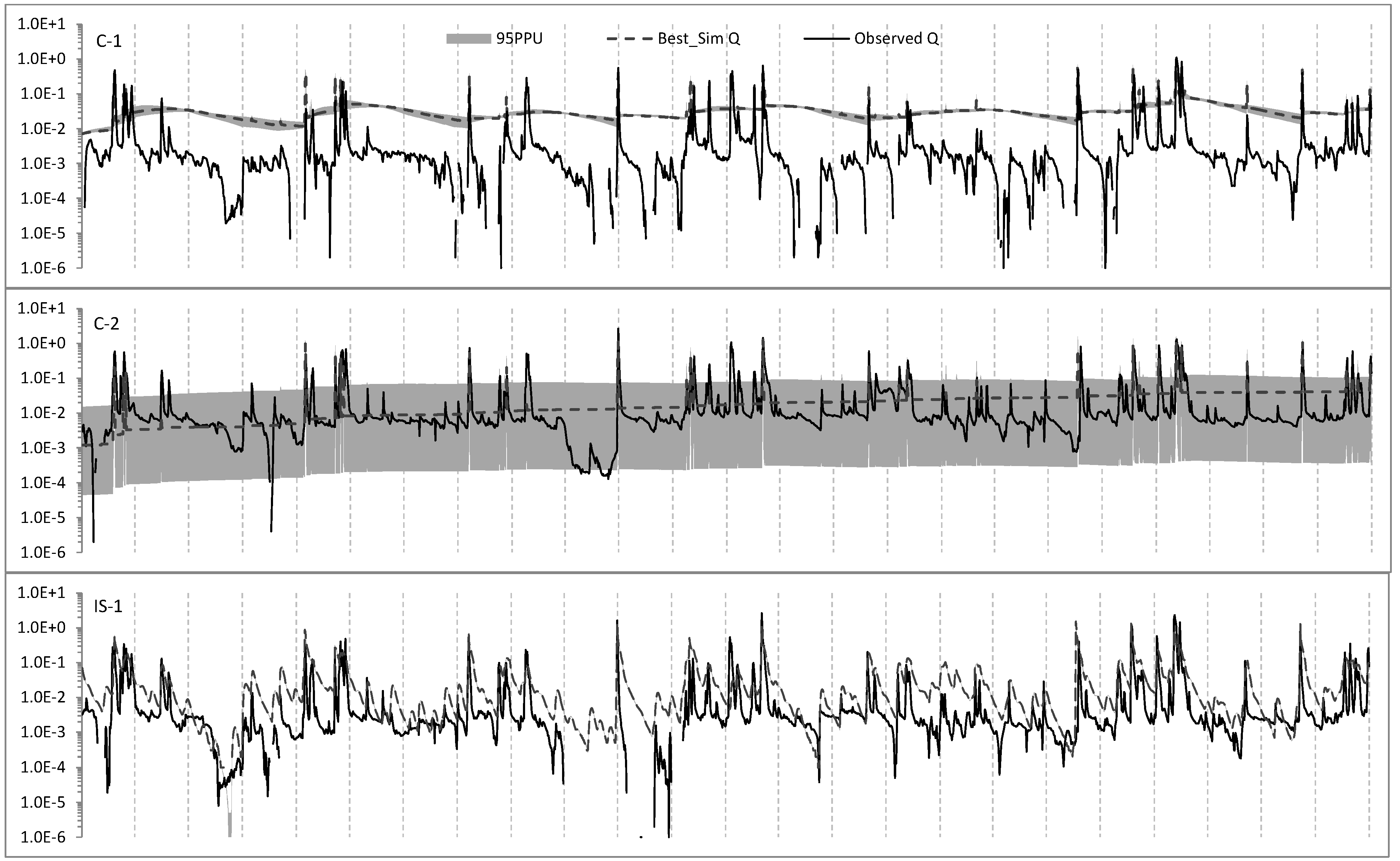
Figure 5 shows 95PPU ranges of streamflow simulations that were obtained from repeated model runs in the best-fit iteration. The median of the 95PPU band was higher than best simulation values in all the catchments other than C-2, indicating that different simulation runs overestimated streamflow and only partly overlaid observed values. However, during periods of high rainfall, the maximum range of simulated 95PPU values followed similar rises in streamflow and observations. During the calibration period, 92% of observations were covered by the repeated simulation runs (95PPU band) for C-2, while the values were simulated poorly for C-1, IS-1 and IS-2 where only 2, 3 and 6% of the observations, respectively were covered by repeated simulation runs. On the other hand, the high coverage of simulations in C-2 does not reflect satisfactory model outputs because of the poor matching of output fluctuations with observations. Further results showed that the width of ranges in simulations (r-index) was also markedly higher in C-2 (0.73) and IS-2 (0.86), indicating a great deal of variability. Having generated an efficient simulation, IS-1 (r-index = 0.02) therefore demonstrated minimum variability with the lowest uncertainty of model outputs, although the modelled datasets slightly overestimated baseflows.

In general, the highest increases in flow yields were both observed and simulated for wet weather conditions (

Table 7. Coefficient of determination (R²) and Nash-Sutcliffe Efficiency (NSE) of incremental changes in observed (Obs.) and simulated (Sim.) daily flows versus respective incremental changes in rainfall for each catchment.

Catchments	Incremental Obs. Q vs. Rain		Incremental Sim. Q vs. Rain
	R2	NSE	R2	NSE
C-1	0.29	−0.83	0.37	0.36
C-2	0.23	0.01	0.49	0.01
IS-1	0.30	−0.44	0.42	0.22
IS-2	0.23	−0.42	0.34	0.22

). There was a relatively close correlation between incremental changes in rain intensity and the corresponding increases in daily simulated flows. The direct impact of rainfall to changes in simulated streamflow is also consistent with other results [67] which pointed to the high impact of precipitation on flow yields in brush management catchments (correlation of R² = 0.75).

Recent climate variations in eastern Australia have been characterized by above average annual rainfalls incorporating high intensity rain events [68]. In addition, global warming trends are predicted to lead to increased rainfall variability especially in existing wetter climates [69]. The SWAT simulations presented here produced reasonable results for high streamflows, the periods when high intensity falls are likely to contribute substantially to increased runoff. Despite limited streamflow and rainfall data in the study area, these simulations are relevant to probable future high flows and potential downstream flow and water quality impacts. Further research is needed to improve SWAT simulations for the extreme hydrological conditions of peak and low streamflows [70]. The SWAT simulation used in our study did not adjust for groundwater changes by combining with MODFLOW, for example [7], as no local aquifer data were available. This, as well as insufficient within-catchment rainfall data, led to overestimation of flow during dry periods and uncertainty in simulations for catchments further from the rain gauge.

4. Conclusions

In this study, a SWAT model was calibrated against continuously recorded streamflow data at gauging stations in the downstream confluence of four adjacent study catchments for the period January 2002 through December 2009, during which period land use/land cover remained almost unchanged. Constraints in data collection and field measurements included the relatively short duration of streamflow and climatic information, especially important in an environment of high interannual rainfall variability. Despite these constraints, results of the study showed that:

• The highest increases in flow yields were both observed and simulated for wet weather conditions;
• Simulations overestimated low flows in three of the four catchments, suggesting that the dynamics of groundwater status would be more accurately simulated by increased numbers of rain gauges and developing relations between saturation-excess and surface water;
• Simulations and observations were closest in the catchment with a rain gauge, confirming requirements for a sufficiently dense network of climate input data to cover spatial variability;
• Longer duration timesteps reduced differences between streamflow simulations and observations;
• High variability in model efficiency between adjacent catchments with similar physical and land use characteristics suggested that small-scale site-specific inputs were necessary.

Robust modelling of streamflow provides an effective tool in contributing to sound management decisions relating to land use and land use changes, especially in headwaters of catchments. In downstream areas, streamflow monitoring assists in managing potential issues in relation to water quality and flood prediction, and for ensuring adequate water supplies for drinking, agricultural and industrial purposes.

References

- Moriasi, D.N.; Arnold, J.G.; van Liew, M.W.; Bingner, R.L.; Harmel, R.D.; Veith, T.L. Model evaluation guidelines for systematic quantification of accuracy in watershed simulations. Trans. ASABE 2007, 50, 885–900. [Google Scholar] [CrossRef]
- Gitau, M.W.; Chiang, L.; Sayeed, M.; Chaubey, I. Watershed Modeling Using Large-Scale Distributed Computing in Condor and SWAT. Simulation 2012, 88, 365–380. [Google Scholar] [CrossRef]
- Shrestha, M.K.; Recknagel, F.; Frizenschaft, J.; Meyer, W. Assessing SWAT models based on single and multi-site calibration for the simulation of flow and nutrient loads in the semi-arid Onkaparinga catchment in South Australia. Agric. Water Manag. 2016, 175, 61–71. [Google Scholar] [CrossRef]
- Shi, Y.Y.; Xu, G.H.; Wang, Y.; Engel, B.A.; Peng, H.; Zhang, W.; Cheng, M.; Dai, M.L. Modelling hydrology and water quality processes in the Pengxi River basin of the Three Gorges Reservoir using the soil and water assessment tool. Agric. Water Manag. 2017, 182, 24–38. [Google Scholar] [CrossRef]
- Karki, R.; Srivastava, P.; Kalin, L.; Lamba, J.; Bosch, D.D. Multi-variable sensitivity analysis, calibration, and validation of a field-scale SWAT model: Building stakeholder trust in hydrologic and water quality modelling. Trans. ASABE 2020, 63, 523–539. [Google Scholar] [CrossRef]
- Noori, N.; Kalin, L.; Isik, S. Water quality prediction using SWAT-ANN coupled approach. J. Hydrol. 2020, 590, 125220. [Google Scholar] [CrossRef]
- Hadjihosseini, M.; Hadjihosseini, H.; Morid, S.; Delavar, M.; Booij, J. Impacts of land use changes and climate variability on transboundary Hirman River using SWAT. J. Water Clim. Chang. 2020, 11, 1695–1711. [Google Scholar] [CrossRef]
- Arnold, J.G.; Kiniry, J.R.; Srinivasan, R.; Williams, J.R.; Haney, E.B.; Neitsch, S.L. Soil and Water Assessment Tool: Input/Output File Documentation (TR-365); Texas Water Resources Institute, Texas A&M University: College Station, TX, USA, 2011. [Google Scholar]
- Santhi, C.; Arnold, J.G.; Williams, J.R.; Dugas, W.A.; Srinivasan, R.; Hauck, L.M. Validation of the SWAT model on a large river basin with point and nonpoint sources. J. Am. Water Resour. Assoc. 2001, 37, 1169–1188. [Google Scholar] [CrossRef]
- Neitsch, S.L.; Arnold, J.G.; Srinivasan, R. Pesticides Fate and Transport Predicted by the Soil and Water Assessment Tool (SWAT); Final Report; Office of Pesticide Programs, Environmental Protection Agency: Washington DC, USA, 2002. [Google Scholar]
- Abbaspour, K.C.; Yang, J.; Maximov, I.; Siber, R.; Bogner, K.; Mieleitner, J.; Zobrist, J.; Srinivasan, R. Modelling hydrology and water quality in the pre-alpine/alpine Thur watershed using SWAT. J. Hydrol. 2007, 333, 413–430. [Google Scholar] [CrossRef]
- Kim, N.W.; Chung, I.M.; Won, Y.S.; Arnold, J.G. Development and application of the integrated SWAT-MODFLOW model. J. Hydrol. 2008, 356, 1–16. [Google Scholar] [CrossRef]
- Schmalz, B.; Fohrer, N. Comparing model sensitivities of different landscapes using the ecohydrological SWAT model. Adv. Geosci. 2009, 21, 91–98. [Google Scholar] [CrossRef] [Green Version]
- Chen, J.; Wu, Y. Advancing representation of hydrologic processes in the Soil and Water Assessment Tool (SWAT) through integration of the TOPographic MODEL (TOPMODEL) features. J. Hydrol. 2012, 420–421, 319–328. [Google Scholar] [CrossRef]
- Dougall, C.; Rohde, K.; Carroll, C.; Millar, G.; Stevens, S. An assessment of land management practices that benchmark water quality targets set at a Neighbourhood Catchment scale using the SWAT model. In Proceedings of the MODSIM Conference, Townsville, Australia: Modelling and Simulation Society of Australia and New Zealand, Townsville, Australia, 13–18 July 2003; Modelling and Simulation Society of Australia and New Zealand Inc.: Canberra, ACT, Australia, 2003; pp. 296–301. [Google Scholar]
- Watson, B.M.; Selvalingam, S.; Ghafouri, M. Evaluation of SWAT for modelling the water balance of the Woady Yaloak River catchment, Victoria. In Proceedings of the MODSIM 2003: International Congress on Modelling and Simulation, Jupiters Hotel and Casino, Integrative Modelling of Biophysical, Social and Economic Systems for Resource Management Solutions, Townsville, Australia, 14–17 July 2003; Modelling and Simulation Society of Australia and New Zealand Inc.: Canberra, ACT, Australia, 2003; pp. 1–6. [Google Scholar]
- Sun, H.; Cornish, P.S. Estimating shallow groundwater recharge in the headwaters of the Liverpool Plains using SWAT. Hydrol. Process. 2005, 19, 795–807. [Google Scholar] [CrossRef]
- Zhang, H.; Wang, B.; Liu, D.L.; Zhang, M.; Leslie, L.M.; Yu, Q. Using an improved SWAT model to simulate hydrological responses to land use change: A case study of a catchment in tropical Australia. J. Hydrol. 2020, 585, 124822. [Google Scholar] [CrossRef]
- Nicholls, N.; Drosdowsky, W.; Lavery, B. Australian rainfall variability and change. Weather 1997, 52, 66–71. [Google Scholar] [CrossRef]
- Dey, R.; Bador, M.; Alexander, L.V.; Lewis, S.C. The drivers of extreme rainfall event timing in Australia. Int. J. Climatol. 2021, 41, 6654–6673. [Google Scholar] [CrossRef]
- Jamshidi, R.; Dragovich, D.; Webb, A.A. Distributed empirical algorithms to estimate catchment scale sediment connectivity and yield in a subtropical region. Hydrol. Process. 2013, 28, 2671–2684. [Google Scholar] [CrossRef]
- Kozlowski, T.T. Soil compaction and growth of woody plants. Scand. J. Forest Res. 1999, 14, 596–619. [Google Scholar] [CrossRef]
- Croke, J.; Mockler, S.; Fogarty, P.; Takken, I. Sediment concentration changes in runoff pathways from a forest road network and the resultant spatial pattern of catchment connectivity. Geomorphology 2005, 68, 257–268. [Google Scholar] [CrossRef]
- Lewis, J.; Mori, S.R.; Keppeler, E.T.; Ziemer, R.R. Impacts of logging on storm peak flows, flow volumes and suspended sediment loads in Caspar Creek, California. In Land Use and Watersheds: Human Influence on Hydrology and Geomorphology in Urban and Forest Areas. Water Science and Application Volume 2; Wigmosta, M.S., Ed.; American Geophysical Union: Washington, DC, USA, 2001; pp. 85–125. [Google Scholar]
- Lenz, B.; Saad, D.; Fitzpatrick, F. Simulation of Ground-Water Flow and Rainfall Runoff with Emphasis on the Effects of Land Cover, Whittlesey Creek, Bayfield County, Wisconsin, 1999–2001. USGS Water-Resources Investigations Report 03–4130. 2003. Available online: http://permanent.access.gpo.gov/waterusgsgov/water.usgs.gov/pubs/wri/wrir-03-4130/index.htm#heading143028536 (accessed on 19 July 2022).
- CBWC (Condamine Balonne Water Committee Inc.). Water quality in the Condamine-Balonne catchment. In Water Quality Monitoring and Information Dissemination Services Project–Final Report; Condamine-Balonne Water Committee Incorporated: Dalby, QLD, Australia, 1999. [Google Scholar]
- Forestry Commission of NSW. Forestry Commission of NSW. Forest types in New South Wales. In Research Note 17; Forestry Commission of NSW: Sydney, NSW, Australia, 1989. [Google Scholar]
- Lunney, D.; Moon, C.; Matthews, A.; Turbill, J. Koala Plan of Management; NSW National Parks and Wildlife Service: Sydney, NSW, Australia, 1999; 95p. [Google Scholar]
- Korsch, R.J. Petrographic variations within thick turbidite sequences: An example from the late Palaeozoic of eastern Australia. Sedimentology 1978, 25, 247–265. [Google Scholar] [CrossRef]
- Gilligan, L.B.; Brownlow, J.W.; Cameron, R.G.; Henley, H.F. Dorrigo-Coffs Harbour 1:250,000 Metallogenic Map; Geological Survey of New South Wales: Sydney, NSW, Australia, 1992. [Google Scholar]
- Milford, H.B. Soil Landscapes of the Dorrigo 1:100 000 Sheet. In Report and Map; Department of Land and Water Conservation: Sydney, NSW, Australia, 1996. [Google Scholar]
- USDA Soil Conservation Service. Estimation of direct runoff from storm rainfall. In National Engineering Handbook; Section IV, Hydrology: Washington, DC, USA, 1972; pp. 4–102. [Google Scholar]
- Neitsch, S.L.; Arnold, J.G.; Kiniry, J.R.; Williams, J.R. Soil and Water Assessment Tool Theoretical Documentation, Version 2005; USDA-ARS Grassland, Soil and Water Research Laboratory: Temple, TX, USA, 2005. [Google Scholar]
- Arnold, J.G.; Srinivasan, R.; Muttiah, R.S.; Williams, J.R. Large area hydrologic modeling and assessment. Part 1: Model development. J. Am. Water Resour. Assoc. 1998, 34, 73–89. [Google Scholar] [CrossRef]
- Gassman, P.W.; Reyes, M.R.; Green, C.H.; Arnold, J.G. The Soil and Water Assessment Tool: Historical Development, Applications, and Future Research Directions. Trans. ASABE 2007, 50, 1211–1250. [Google Scholar] [CrossRef] [Green Version]
- Gitau, M.W.; Gburek, W.J.; Bishop, P.L. Use of the SWAT model to quantify water quality effects of agricultural BMPs at the farm-scale level. Trans ASABE 2008, 51, 1925–1936. [Google Scholar] [CrossRef]
- Neitsch, S.L.; Arnold, J.G.; Kiniry, J.R.; Williams, J.R. Soil and Water Assessment Tool-Theoretical Documentation, Version 2009; U.S. Dept. of Agriculture, Agriculture Research Service, Grassland, Soil, and Water Research Laboratory: Temple, TX, USA, 2011; Available online: http://swatmodel.tamu.edu/documentation (accessed on 22 June 2022).
- ESRI (Environmental Systems Research Institute, Inc.). ArcGIS Desktop: Release 10.0. Redlands; Environmental Systems Research Institute: Redlands, CA, USA, 2011. [Google Scholar]
- USDA Natural Resources Conservation Service. National Engineering Handbook, Part 630, Hydrology, Chapter 7; Hydrologic Soil Groups, NEH 630.07: Washington, DC, USA, 2009. [Google Scholar]
- Jamshidi, R.; Dragovich, D.; Webb, A. Catchment scale geostatistical simulation and uncertainty of soil erodibility using sequential Gaussian simulation. Environ. Earth Sci. 2014, 71, 4965–4976. [Google Scholar]
- Australian Government, Bureau of Meteorology. Daily Maximum Temperature, Dorrigo (Old Coramba Road). 2022. Available online: http://www.bom.gov.au/jsp/ncc/cdio/weatherData/av?p_nccObsCode=122&p_display_type=dailyData-File&p_startYear=&p_c=&p_stn_num=059140 (accessed on 19 July 2022).
- Australian Government, Bureau of Meteorology. Daily Minimum Temperature, Dorrigo (Old Coramba Road). 2022. Available online: http://www.bom.gov.au/jsp/ncc/cdio/weatherData/av?p_nccObsCode=123&p_display_type=dailyDataFile&p_startYear=&p_c=&p_stn_num=059140 (accessed on 19 July 2022).
- Zhou, J.; Liu, Y.; Guo, H.; He, D. Combining the SWAT model with sequential uncertainty fitting algorithm for streamflow prediction and uncertainty analysis for the Lake Dianchi Basin, China. Hydrol. Process. 2012, 28, 521–533. [Google Scholar] [CrossRef]
- Tolson, B.A.; Shoemaker, C.A. Cannonsville reservoir watershed swat2000 model development, calibration and validation. J. Hydrol. 2007, 337, 68–86. [Google Scholar] [CrossRef]
- Rouholahnejad, E.; Abbaspour, K.C.; Vejdani, M.; Srinivasan, R.; Schulin, R.; Lehmann, A. A parallelization framework for calibration of hydrological models. Environ. Model. Softw. 2012, 31, 28–36. [Google Scholar] [CrossRef]
- Krause, P.; Boyle, D.P.; Bäse, F. Comparison of different efficiency criteria for hydrological model assessment. Adv. Geosci. 2005, 5, 89–97. [Google Scholar] [CrossRef] [Green Version]
- Nash, J.E.; Sutcliffe, J.V. River flow forecasting through conceptual models: Part 1. A discussion of principles. J. Hydrol. 1970, 10, 282–290. [Google Scholar] [CrossRef]
- van Griensven, A.; Meixner, T.; Grunwald, S.; Bishop, T.; Di Luzio, M.; Srinivasan, R.A. Global Sensitivity Analysis Method for the Parameters of Multi-Variable Watershed Models. J. Hydrol. 2006, 324, 10–23. [Google Scholar] [CrossRef]
- Yang, J.; Reichert, P.; Abbaspour, K.C.; Xia, J.; Yang, H. Comparing uncertainty analysis techniques for a SWAT application to the Chaohe Basin in China. J. Hydrol. 2008, 358, 1–23. [Google Scholar] [CrossRef]
- Mbonimpa, E.; Yuan, Y.; Mehaffey, M.; Jackson, M. SWAT Model Application to Assess the Impact of Intensive Corn-farming on Runoff, Sediments and Phosphorous loss from an Agricultural Watershed in Wisconsin. J. Water Resour. Prot. 2012, 4, 423–431. [Google Scholar] [CrossRef] [Green Version]
- Risal, A.; Parajuli, P.B.; Dash, P.; Ouyang, Y.; Linhoss, A. Sensitivity of hydrology and water quality to variation in land use and land cover data. Agric. Water Manag. 2020, 241, 106366. [Google Scholar] [CrossRef]
- Luo, Y.; Zhang, M. Management-oriented sensitivity analysis for pesticide transport in watershed-scale water quality modeling using SWAT. Environ. Pollut. 2009, 157, 3370–3378. [Google Scholar] [CrossRef] [PubMed]
- Hoang, L.; Schneiderman, E.M.; Moore, K.E.B.; Mukundan, R.; Owens, E.M.; Steenhuis, T.S. Predicting saturation-excess runoff distribution with a lumped hillslope model: SWAT-HS. Hydrol. Process. 2017, 31, 2226–2243. [Google Scholar] [CrossRef]
- White, E.D.; Easton, Z.M.; Fuka, D.R.; Collick, A.S.; Adgo, E.; McCartney, M.; Awulachew, S.B.; Selassie, Y.G.; Steenhuis, T.S. Development and application of a physically based landscape water balance in the SWAT model. Hydrol. Process. 2011, 25, 915–925. [Google Scholar] [CrossRef]
- Kumar, S.; Singh, A.; Shrestha, D.P. Modelling spatially distributed surface runoff generation using SWAT-VSA: A case study in a watershed of the north-west Himalayan landscape. Model. Earth Syst. Environ. 2016, 2, 1–11. [Google Scholar] [CrossRef] [Green Version]
- Ndomba, P.; Mtalo, F.; Killingtveit, A. SWAT model application in a data scarce tropical complex catchment in Tanzania. Phys. Chem. Earth 2008, 33, 626–632. [Google Scholar] [CrossRef]
- Molina-Navarro, E.; Bailey, R.T.; Andersen, H.E.; Thodsen, H.; Nielsen, A.; Park, S.; Jensen, J.S.; Jensen, J.B.; Trolle, D. Comparison of abstraction scenarios simulated by SWAT and SWAT-MODFLOW. Hydrol. Sci. J. 2019, 64, 434–454. [Google Scholar] [CrossRef]
- Bailey, R.T.; Bieger, K.; Arnold, J.G.; Bosch, D.D. A New Physically-Based Spatially-Distributed Groundwater Flow Module for SWAT+. Hydrology 2020, 7, 75. [Google Scholar] [CrossRef]
- Wang, C.; Gomez-Velez, J.D.; Wilson, J.L. Dynamic coevolution of baseflow and multiscale groundwater flow system during prolonged droughts. J. Hydrol. 2022, 609, 127657. [Google Scholar] [CrossRef]
- Pang, S.; Wang, X.; Melching, C.S.; Feger, K.-H. Development and testing of a modified SWAT model based on slope condition and precipitation intensity. J. Hydrol. 2020, 588, 125098. [Google Scholar] [CrossRef]
- Almeida, R.A.; Pereira, S.B.; Pinto, D.B. Calibration and validation of the SWAT hydrological model for the Mucuri River Basin. Eng. Agrícola 2018, 38, 55–63. [Google Scholar] [CrossRef] [Green Version]
- Tan, M.L.; Yang, X. Effect of rainfall station density, distribution and missing values on SWAT outputs in tropical region. J. Hydrol. 2020, 584, 124660. [Google Scholar] [CrossRef]
- Bumgarner, J.R.; Thompson, F.E. Simulation of Streamflow and the Effects of Brush Management on Water Yields in the Upper Guadalupe River Watershed, South-Central Texas, 1995–2010. U.S.; Geological Survey Scientific Investigations Report 2012–5051; USGS: Reston, VA, USA, 2012. [Google Scholar]
- Afinowicz, J.D.; Munster, C.L.; Wilcox, B.P. Modeling effects of brush management on the rangeland water budget–Edwards Plateau, Texas. J. Am. Water Resour. Assoc. 2005, 41, 181–193. [Google Scholar] [CrossRef]
- Cerkasova, N.; Umgiesser, G.; Erturk, A. Development of a hydrology and water quality model for a large transboundary river watershed to investigate the impacts of climate change–A SWAT application. Ecol. Eng. 2018, 124, 99–115. [Google Scholar] [CrossRef]
- Malik, M.A.; Dar, A.Q.; Jain, M.K. Modelling streamflow using the SWAT model and multi-site calibration utilizing SUFI-2 of SWAT-CUP model for high altitude catchments, NW Himalayas. Modeling Earth Syst. Environ. 2022, 8, 1203–1213. [Google Scholar] [CrossRef]
- Bednarz, S.T.; Dybala, T.; Muttiah, R.S.; Rosenthal, W.; Dugas, W.A. Brush Management/Water Yield Feasibility Studies for Eight Watersheds in Texas; Texas Water Resources Institute Report TR-182; Texas A&M University: College Station, TX, USA, 2000. [Google Scholar]
- Australian Government, Bureau of Meteorology. Heavy Rainfall Events Are Becoming More Intense. 2022. Available online: http://www.bom.gov.au/state-of-the-climate/australias-changing-climate.shtml (accessed on 23 November 2022).
- Deb, P.; Kiem, A.S.; Willgoose, G. A linked surface-groundwater modelling approach to more realistically simulate rainfall-runoff non-stationarity in semi-arid regions. J. Hydrol. 2019, 575, 273–291. [Google Scholar] [CrossRef]
- Tan, M.L.; Gassman, P.W.; Yang, X.; Haywood, J. A review of SWAT applications, performance and future needs for simulation of hydro-climatic extremes. Adv. Water Resour. 2020, 143, 103662. [Google Scholar] [CrossRef]