
Multilayer Perceptron and Their Comparison with Two Nature-Inspired Hybrid Techniques of Biogeography-Based Optimization (BBO) and Backtracking Search Algorithm (BSA) for Assessment of Landslide Susceptibility
 ,
,  ,
,
Abstract
:1. Introduction
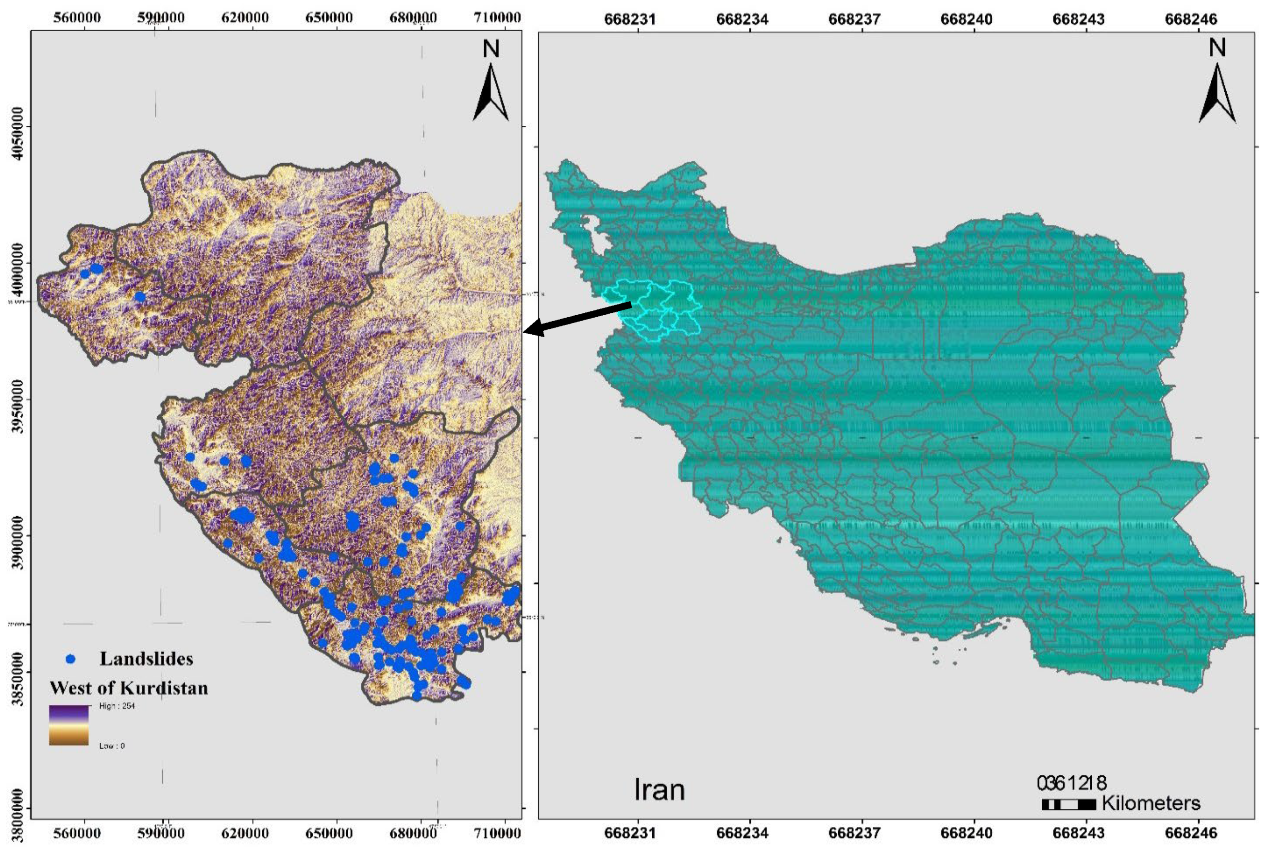
2. Review of Case Study
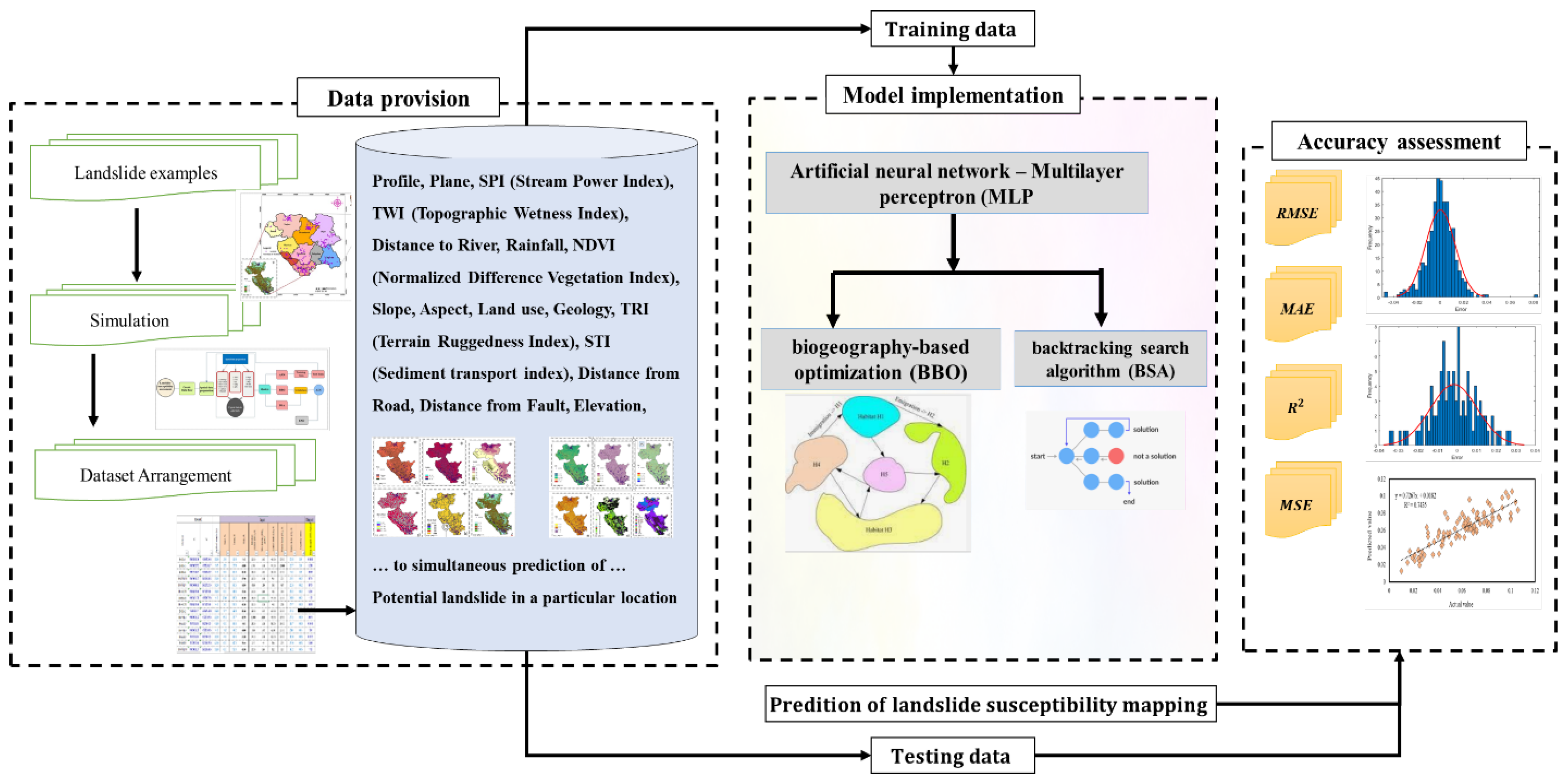
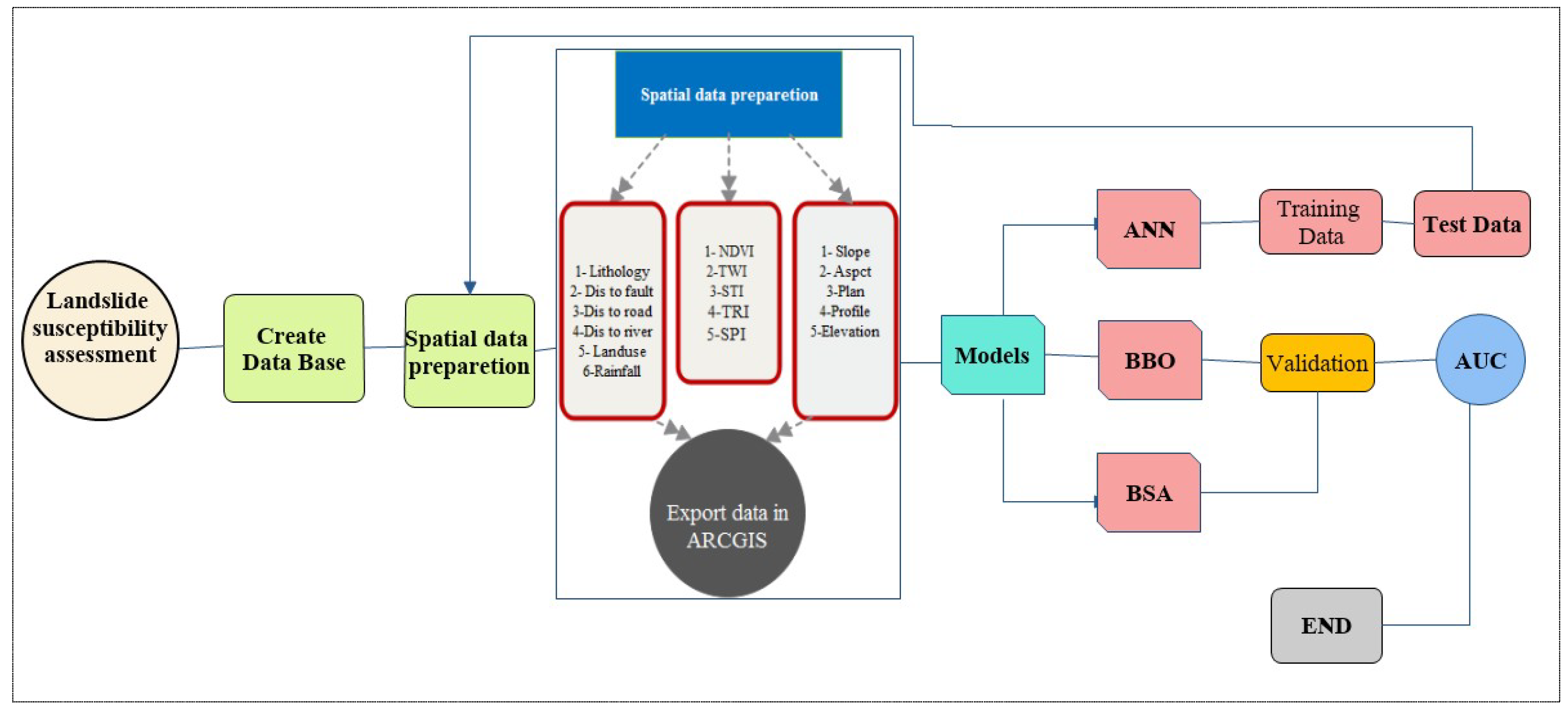
3. Methodology
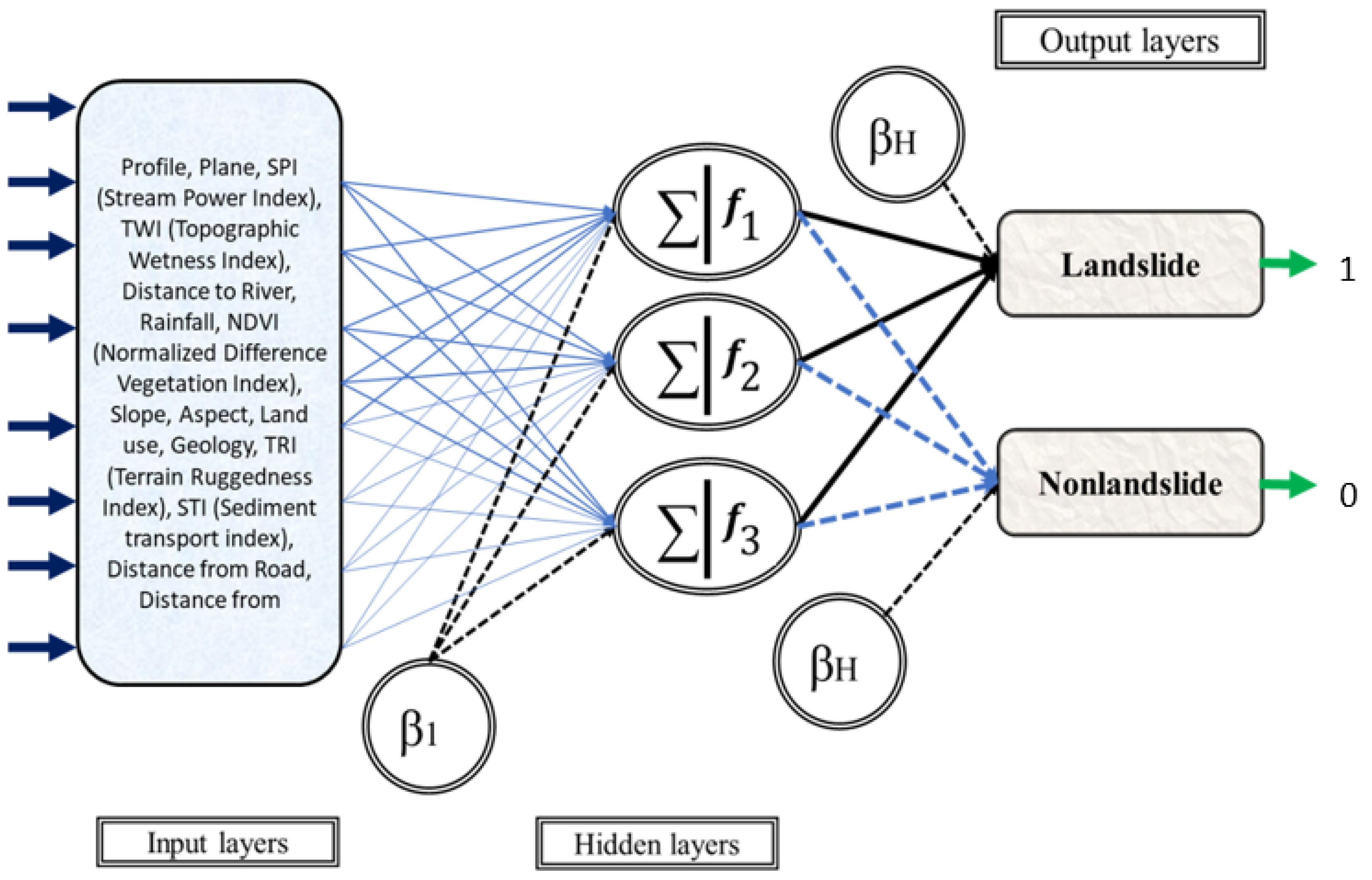
3.1. Artificial Neural Network
3.2. Hybrid Model Development
- (a)
- Determining the ideal structure of the ANN model: we are aware that the structure of the ANN has a significant impact on the accuracy of its predictions [41]. As the model’s backbone, it should be optimized in hybrid models [39]. The network with several processors in the intermediate layer and a Tansig activation function is the optimal solution, as determined by a trial-and-error procedure applied to various tested configurations.
- (b)
- Specify the problem function and use the BBO-MLP and BSA-MLP models.
- (c)
- Specify precise parameters such as population size, number of iterations, and goal function.
- (d)
- Minimizing inaccuracy by modifying the ANN’s weights and biases
- (e)
- Storing the optimum solution when a termination condition is met.
3.2.1. Biogeography-Based Optimization (BBO)
- (1)
- BBO parameters require configuration, which consists of emanating a representative method for habitats, that is concerned with hanging and initializing the highest migration rate, transformation rate, and elitism parameter.
- (2)
- Create a random set of habitats based on the possible solution sets and initialize them.
- (3)
- Each habitat’s migration and emigration rates can be determined by utilizing its HSI.
- (4)
- Migrate in a random fashion to change the environment of each special habitat. The HSIs were then computed again.
- (5)
- Each habitat should be assigned a mutation rate based on the number of species present.
- (6)
- Random mutations should be applied to every non-light habitat. It was then recalculated for each individual HSI.
- (7)
- To begin the next iteration, go to step one (3). Repeat for as many generations as necessary till you have come up with the right answer.
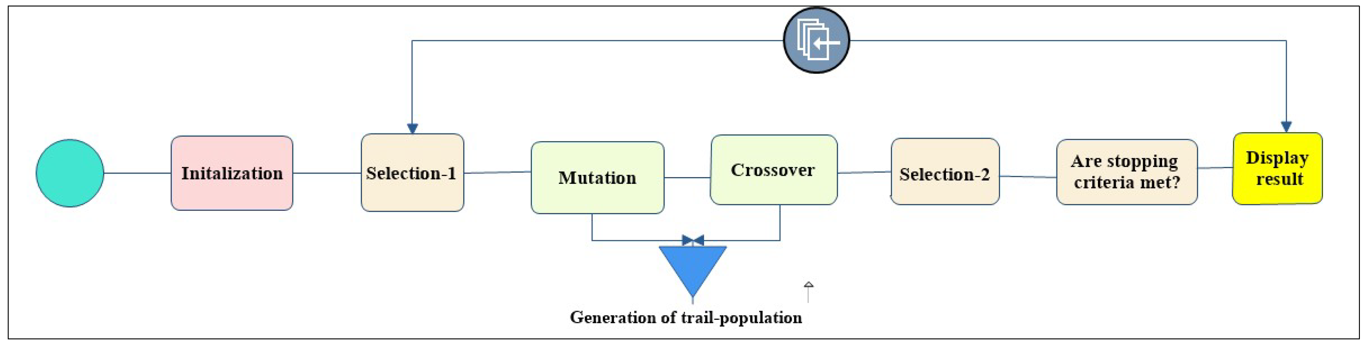
3.2.2. Backtracking Search Algorithm (BSA)
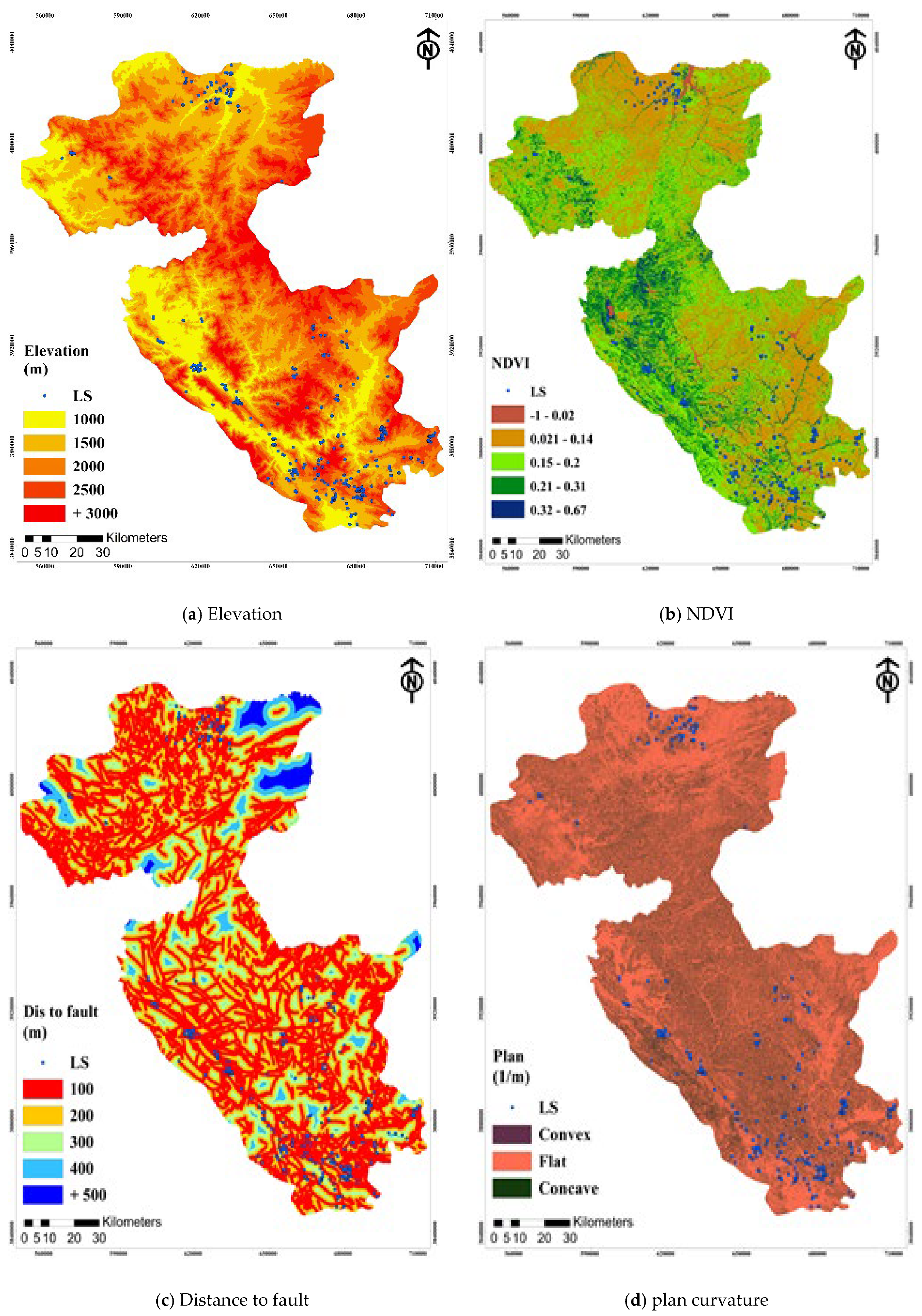
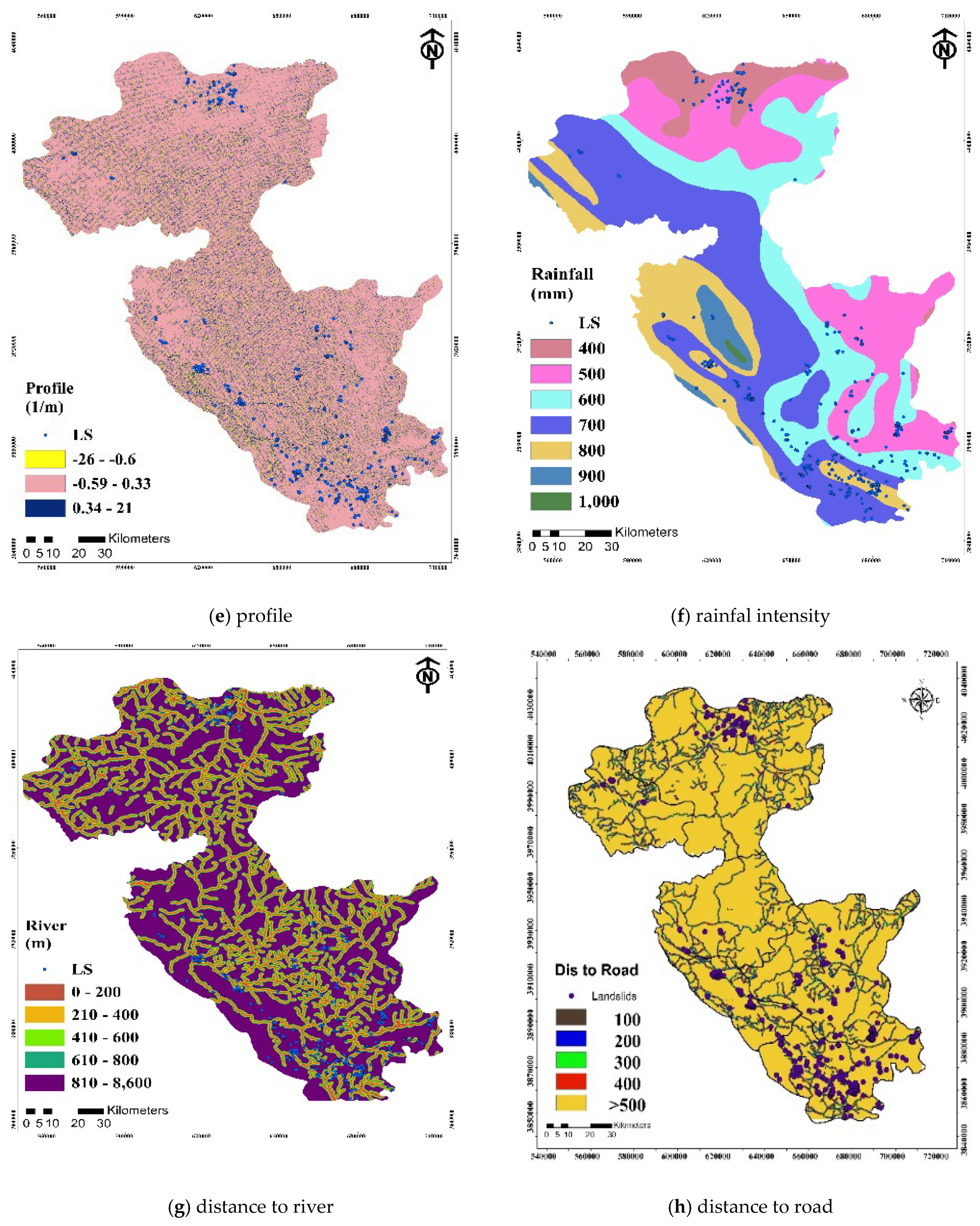
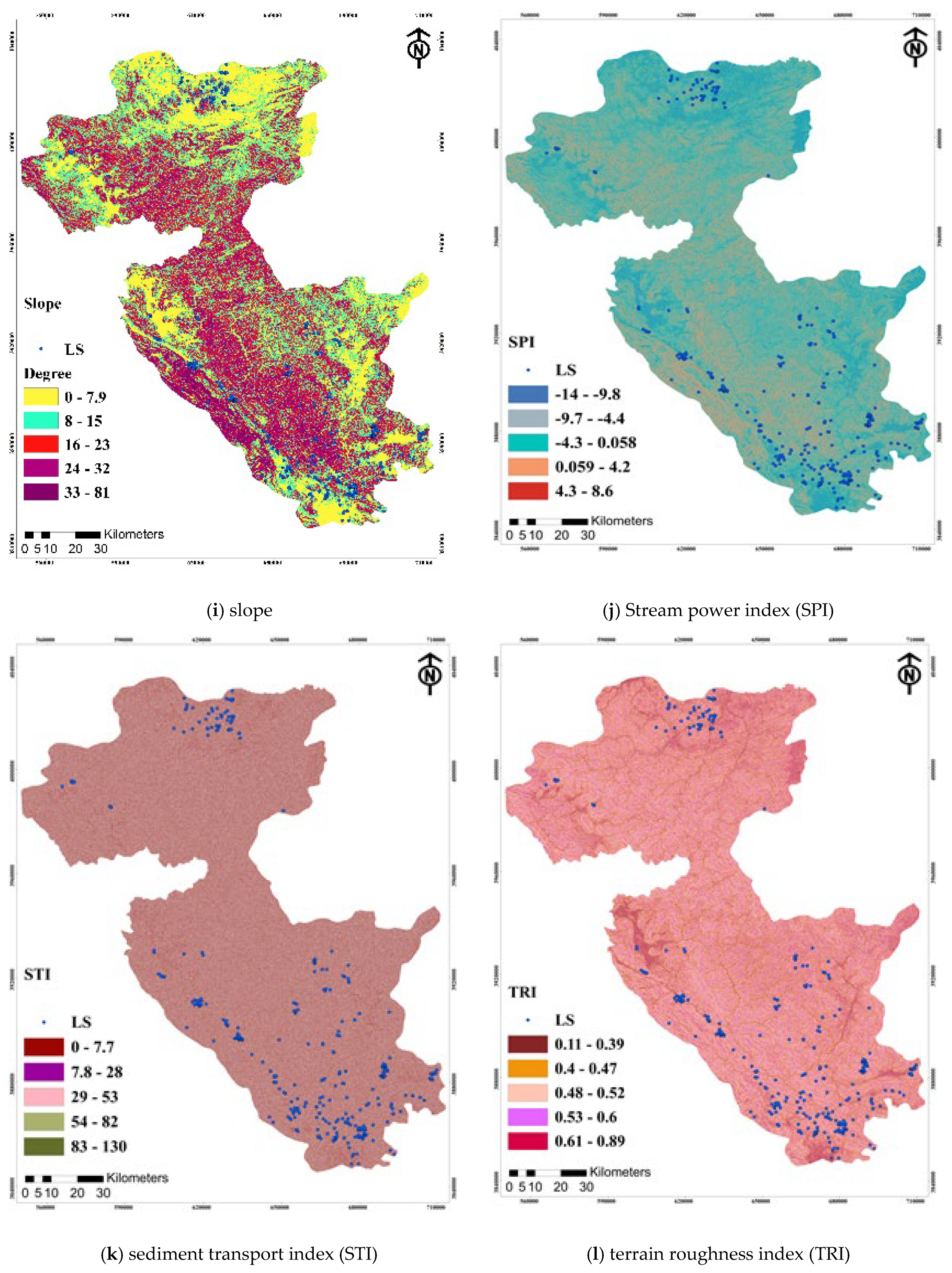
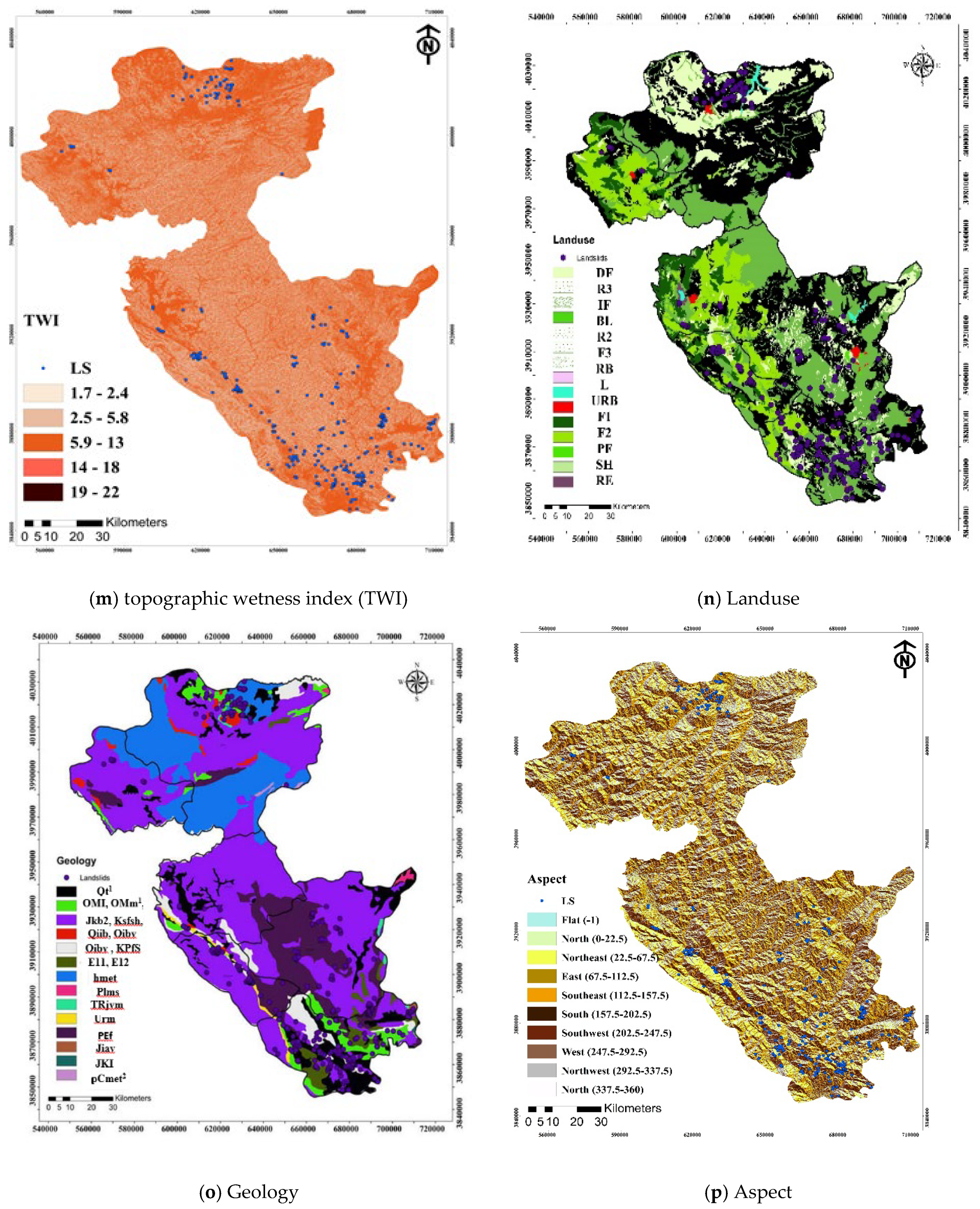
3.3. Landslide Inventory Map (LIM) and Landslide Conditioning Factors
4. Results and Discussion
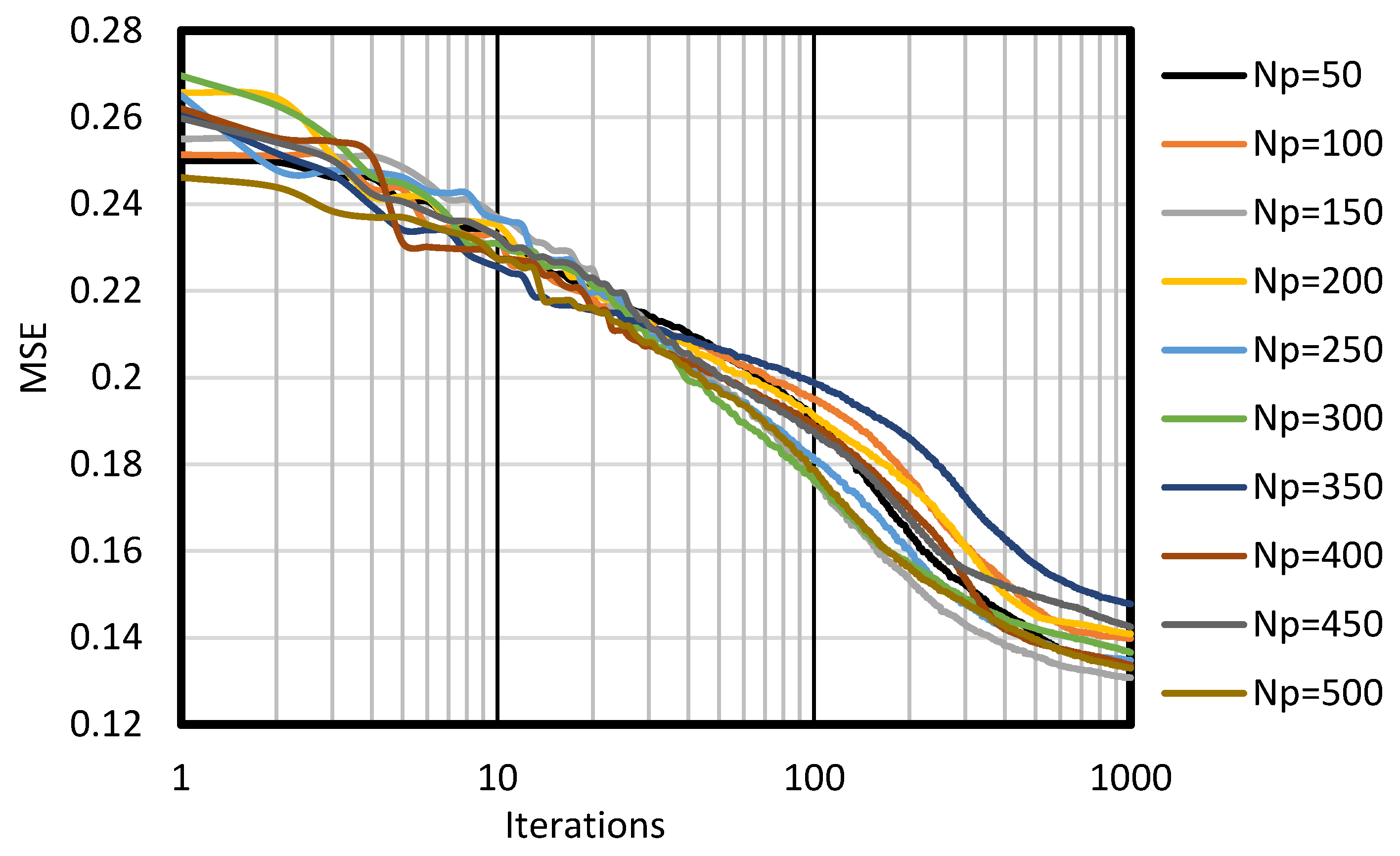
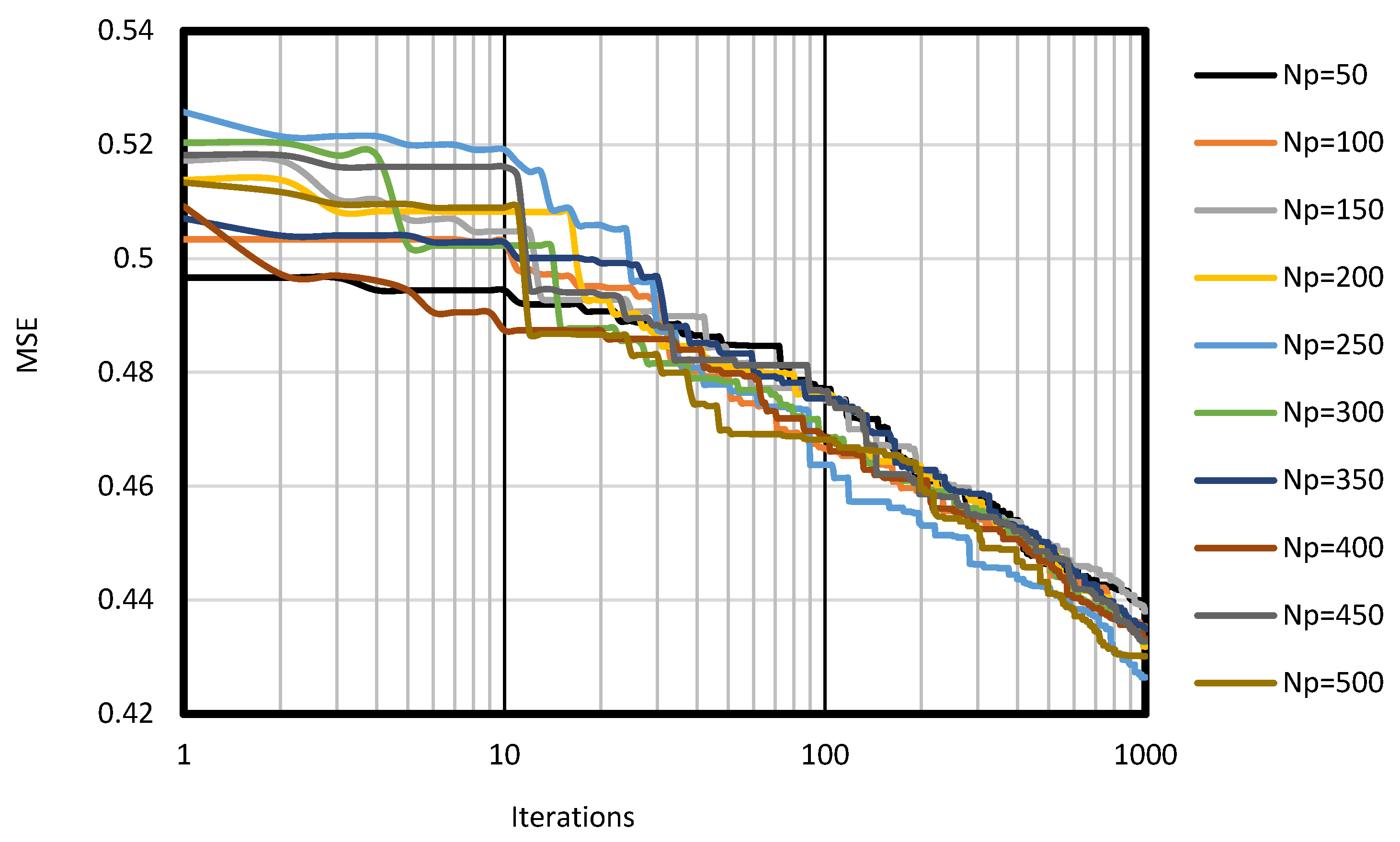
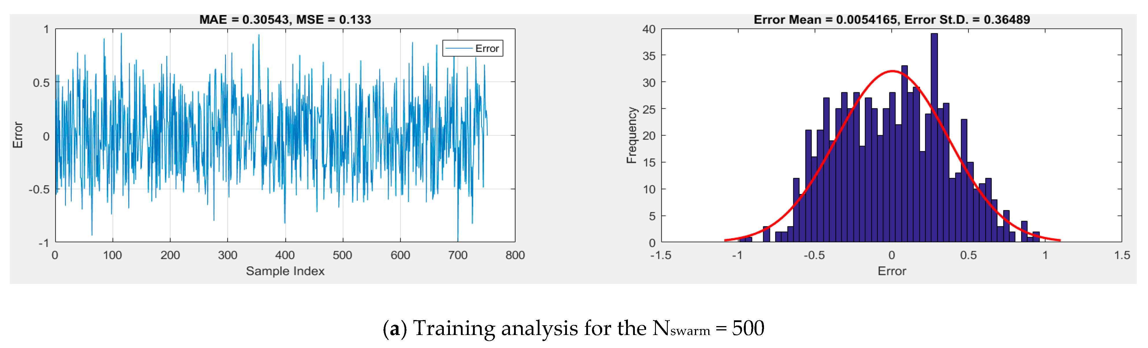
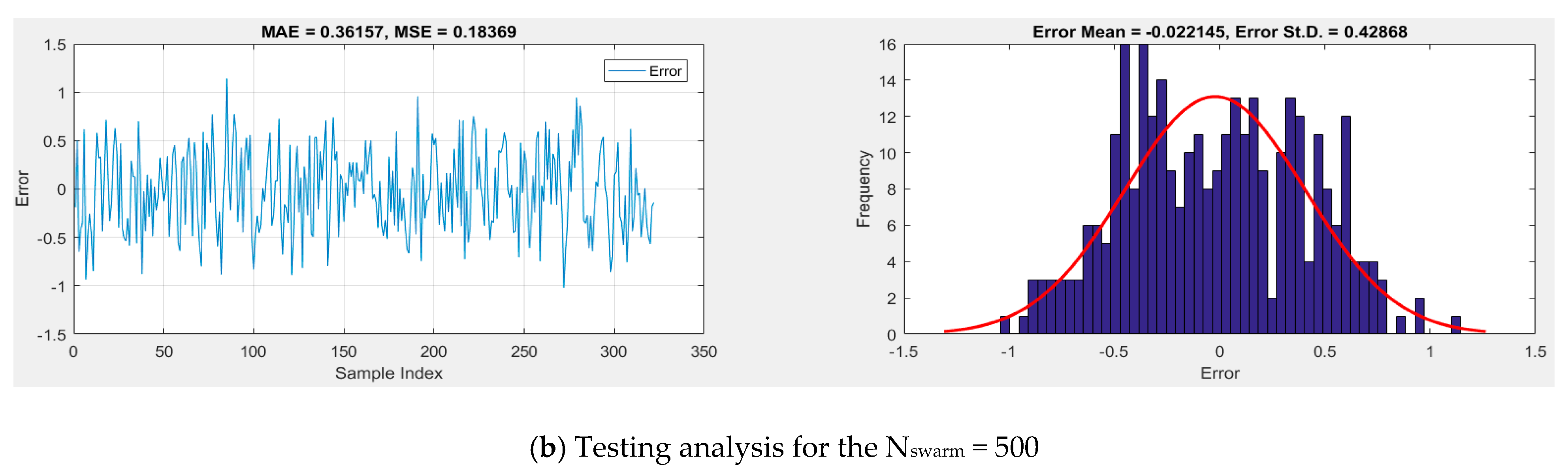
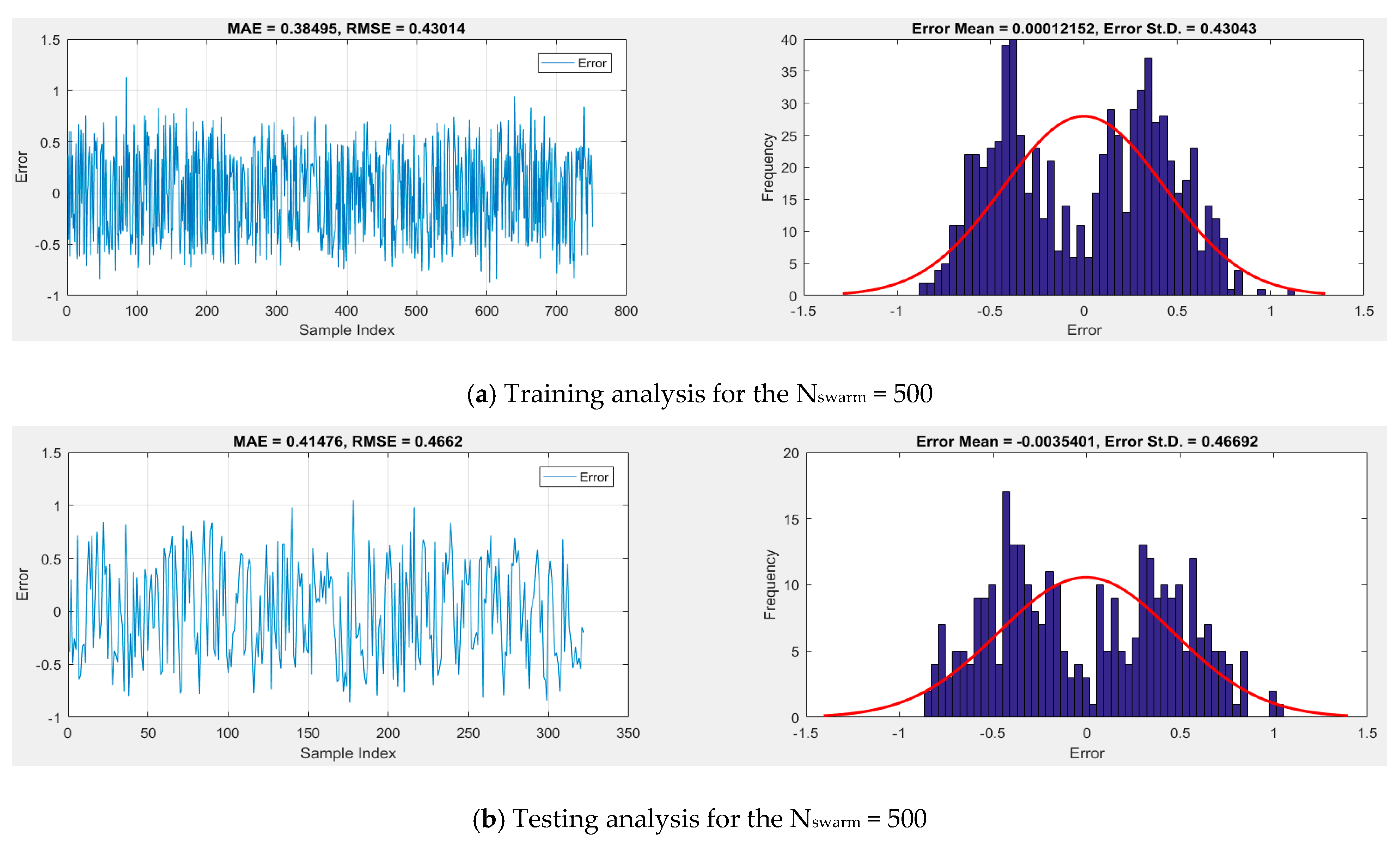
Error Analysis
5. Conclusions
Author Contributions
Funding
Institutional Review Board Statement
Informed Consent Statement
Data Availability Statement
Acknowledgments
Conflicts of Interest
References
- Zhao, Y.; Hu, H.; Bai, L.; Tang, M.; Chen, H.; Su, D. Fragility Analyses of Bridge Structures Using the Logarithmic Piecewise Function-Based Probabilistic Seismic Demand Model. Sustainability 2021, 13, 7814. [Google Scholar] [CrossRef]
- Li, Q.; Song, D.; Yuan, C.; Nie, W. An image recognition method for the deformation area of open-pit rock slopes under variable rainfall. Measurement 2021, 188, 110544. [Google Scholar] [CrossRef]
- Huang, S.; Lyu, Y.; Sha, H.; Xiu, L. Seismic performance assessment of unsaturated soil slope in different groundwater levels. Landslides 2021, 18, 2813–2833. [Google Scholar] [CrossRef]
- Wang, G.; Zhao, B.; Lan, R.; Liu, D.; Wu, B.; Li, Y.; Li, Q.; Zhou, H.; Liu, M.; Liu, W.; et al. Experimental Study on Failure Model of Tailing Dam Overtopping under Heavy Rainfall. Lithosphere 2022, 5922501. [Google Scholar] [CrossRef]
- Fang, X.; Wang, Q.; Wang, J.; Xiang, Y.; Wu, Y.; Zhang, Y. Employing extreme value theory to establish nutrient criteria in bay waters: A case study of Xiangshan Bay. J. Hydrol. 2021, 603, 127146. [Google Scholar] [CrossRef]
- Gao, C.; Hao, M.; Chen, J.; Gu, C. Simulation and design of joint distribution of rainfall and tide level in Wuchengxiyu Region, China. Urban Clim. 2021, 40, 101005. [Google Scholar] [CrossRef]
- Quan, Q.; Liang, W.; Yan, D.; Lei, J. Influences of joint action of natural and social factors on atmospheric process of hydrological cycle in Inner Mongolia, China. Urban Clim. 2022, 41, 101043. [Google Scholar] [CrossRef]
- Zhao, L.; Du, M.; Du, W.; Guo, J.; Liao, Z.; Kang, X.; Liu, Q. Evaluation of the Carbon Sink Capacity of the Proposed Kunlun Mountain National Park. Int. J. Environ. Res. Public Health 2022, 19, 9887. [Google Scholar] [CrossRef]
- Zhao, Y.; Joseph, A.J.J.M.; Zhang, Z.; Ma, C.; Gul, D.; Schellenberg, A.; Hu, N. Deterministic snap-through buckling and energy trapping in axially-loaded notched strips for compliant building blocks. Smart Mater. Struct. 2019, 29, 02LT03. [Google Scholar] [CrossRef]
- Zhang, Y.; Luo, J.; Li, J.; Mao, D.; Zhang, Y.; Huang, Y.; Yang, J. Fast Inverse-Scattering Reconstruction for Airborne High-Squint Radar Imagery Based on Doppler Centroid Compensation. IEEE Trans. Geosci. Remote Sens. 2021, 60, 1–17. [Google Scholar] [CrossRef]
- Yan, B.; Ma, C.; Zhao, Y.; Hu, N.; Guo, L. Geometrically Enabled Soft Electroactuators via Laser Cutting. Adv. Eng. Mater. 2019, 21, 1900664. [Google Scholar] [CrossRef]
- Bui, D.T.; Moayedi, H.; Kalantar, B.; Osouli, A.; Pradhan, B.; Nguyen, H.; A Rashid, A.S. A Novel Swarm Intelligence—Harris Hawks Optimization for Spatial Assessment of Landslide Susceptibility. Sensors 2019, 19, 3590. [Google Scholar] [CrossRef] [Green Version]
- Khezri, S.; Dehrashid, A.A.; Nasrollahizadeh, B.; Moayedi, H.; Dehrashid, H.A.; Azadi, H.; Scheffran, J. Prediction of landslides by machine learning algorithms and statistical methods in Iran. Environ. Earth Sci. 2022, 81, 1–22. [Google Scholar] [CrossRef]
- Moayedi, H.; Mehrabi, M.; Mosallanezhad, M.; Rashid, A.S.A.; Pradhan, B. Modification of landslide susceptibility mapping using optimized PSO-ANN technique. Eng. Comput. 2019, 35, 967–984. [Google Scholar] [CrossRef]
- Moayedi, H.; Osouli, A.; Bui, D.T.; Foong, L.K. Spatial Landslide Susceptibility Assessment Based on Novel Neural-Metaheuristic Geographic Information System Based Ensembles. Sensors 2019, 19, 4698. [Google Scholar] [CrossRef] [Green Version]
- Nguyen, H.; Mehrabi, M.; Kalantar, B.; Moayedi, H.; Abdullahi, M.M. Potential of hybrid evolutionary approaches for assessment of geo-hazard landslide susceptibility mapping. Geomat. Nat. Hazards Risk 2019, 10, 1667–1693. [Google Scholar] [CrossRef] [Green Version]
- Xi, W.; Li, G.; Moayedi, H.; Nguyen, H. A particle-based optimization of artificial neural network for earthquake-induced landslide assessment in Ludian county, China. Geomat. Nat. Hazards Risk 2019, 10, 1750–1771. [Google Scholar] [CrossRef] [Green Version]
- Saremi, S.; Mirjalili, S.; Lewis, A. Grasshopper Optimisation Algorithm: Theory and application. Adv. Eng. Softw. 2017, 105, 30–47. [Google Scholar] [CrossRef] [Green Version]
- Mirjalili, S.; Lewis, A. S-shaped versus V-shaped transfer functions for binary Particle Swarm Optimization. Swarm Evol. Comput. 2013, 9, 1–14. [Google Scholar] [CrossRef]
- Hashimoto, H.; Yagiura, M.; Ibaraki, T. An iterated local search algorithm for the time-dependent vehicle routing problem with time windows. Discret. Optim. 2008, 5, 434–456. [Google Scholar] [CrossRef]
- Glover, F. Tabu search—Part I. ORSA J. Comput. 1989, 1, 190–206. [Google Scholar] [CrossRef] [Green Version]
- Eberhart, R.; Kennedy, J. In A new optimizer using particle swarm theory, MHS’95. In Proceedings of the Sixth International Symposium on Micro Machine and Human Science, Nagoya, Japan, 4–6 October 1995; pp. 39–43. [Google Scholar]
- Storn, R.; Price, K. Differential evolution—A simple and efficient heuristic for global optimization over continuous spaces. J. Glob. Optim. 1997, 11, 341–359. [Google Scholar] [CrossRef]
- Eiben, A.; Schippers, C. On Evolutionary Exploration and Exploitation. Fundam. Inform. 1998, 35, 35–50. [Google Scholar] [CrossRef]
- Zhang, L.; Huang, M.; Li, M.; Lu, S.; Yuan, X.; Li, J. Experimental Study on Evolution of Fracture Network and Permeability Characteristics of Bituminous Coal Under Repeated Mining Effect. Nat. Resour. Res. 2021, 31, 463–486. [Google Scholar] [CrossRef]
- Li, J.; Wang, Y.; Nguyen, X.; Zhuang, X.; Li, J.; Querol, X.; Li, B.; Moreno, N.; Hoang, V.; Cordoba, P.; et al. First insights into mineralogy, geochemistry, and isotopic signatures of the Upper Triassic high-sulfur coals from the Thai Nguyen Coal field, NE Vietnam. Int. J. Coal Geol. 2022, 261, 104097. [Google Scholar] [CrossRef]
- Balogun, A.-L.; Rezaie, F.; Pham, Q.B.; Gigović, L.; Drobnjak, S.; Aina, Y.A.; Panahi, M.; Yekeen, S.T.; Lee, S. Spatial prediction of landslide susceptibility in western Serbia using hybrid support vector regression (SVR) with GWO, BAT and COA algorithms. Geosci. Front. 2020, 12, 101104. [Google Scholar] [CrossRef]
- Tian, H.; Wang, Y.; Chen, T.; Zhang, L.; Qin, Y. Early-Season Mapping of Winter Crops Using Sentinel-2 Optical Imagery. Remote Sens. 2021, 13, 3822. [Google Scholar] [CrossRef]
- Li, J.; Xu, K.; Chaudhuri, S.; Yumer, E.; Zhang, H.; Guibas, L. GRASS: Generative Recursive Autoencoders for Shape Structures. ACM Trans. Graph. 2017, 36, 1–14. [Google Scholar] [CrossRef]
- Naji, H.R.; Shadravan, S.; Jafarabadi, H.M.; Momeni, H. Accelerating sailfish optimization applied to unconstrained optimization problems on graphical processing unit. Eng. Sci. Technol. Int. J. 2021, 32, 101077. [Google Scholar] [CrossRef]
- Chen, W.; Chen, Y.; Tsangaratos, P.; Ilia, I.; Wang, X. Combining Evolutionary Algorithms and Machine Learning Models in Landslide Susceptibility Assessments. Remote Sens. 2020, 12, 3854. [Google Scholar] [CrossRef]
- Zhao, Y.; Hu, H.; Song, C.; Wang, Z. Predicting compressive strength of manufactured-sand concrete using conventional and metaheuristic-tuned artificial neural network. Measurement 2022, 194, 110993. [Google Scholar] [CrossRef]
- Zhao, Y.; Moayedi, H.; Bahiraei, M.; Foong, L.K. Employing TLBO and SCE for optimal prediction of the compressive strength of concrete. Smart Struct. Syst. 2020, 26, 753–763. [Google Scholar]
- Yinghao, Z.; Xiaolin, Z.; Loke Kok, F. Predicting the splitting tensile strength of concrete using an equilibrium optimization model. Steel and Composite Structures. Int. J. 2021, 39, 81–93. [Google Scholar]
- Zhao, Y.; Foong, L.K. Predicting electrical power output of combined cycle power plants using a novel artificial neural network optimized by electrostatic discharge algorithm. Measurement 2022, 198, 111405. [Google Scholar] [CrossRef]
- Wu, P.; Liu, A.; Fu, J.; Ye, X.; Zhao, Y. Autonomous surface crack identification of concrete structures based on an improved one-stage object detection algorithm. Eng. Struct. 2022, 272, 114962. [Google Scholar] [CrossRef]
- Zhao, Y.; Wang, Z. Subset simulation with adaptable intermediate failure probability for robust reliability analysis: An unsupervised learning-based approach. Struct. Multidiscip. Optim. 2022, 65, 1–22. [Google Scholar] [CrossRef]
- Zhao, Y.; Yan, Q.; Yang, Z.; Yu, X.; Jia, B. A Novel Artificial Bee Colony Algorithm for Structural Damage Detection. Adv. Civ. Eng. 2020, 2020, 3743089. [Google Scholar] [CrossRef] [Green Version]
- Loke Kok, F.; Yinghao, Z.; Chengzong, B.; Chengyong, X. Efficient metaheuristic-retrofitted techniques for concrete slump simulation. Smart Structures and Systems. Smart Struct. Syst. 2021, 27, 745–759. [Google Scholar]
- Zhang, K.; Kimball, J.S.; Zhao, M.; Oechel, W.; Cassano, J.; Running, S.W. Sensitivity of pan-Arctic terrestrial net primary productivity simulations to daily surface meteorology from NCEP-NCAR and ERA-reanalyses. J. Geophys. Res. Atmos. 2007, 112, G01011. [Google Scholar] [CrossRef]
- Ikram, R.M.A.; Dai, H.-L.; Ewees, A.A.; Shiri, J.; Kisi, O.; Zounemat-Kermani, M. Application of improved version of multi verse optimizer algorithm for modeling solar radiation. Energy Rep. 2022, 8, 12063–12080. [Google Scholar] [CrossRef]
- Simon, D. Biogeography-Based Optimization. IEEE Trans. Evol. Comput. 2008, 12, 702–713. [Google Scholar] [CrossRef] [Green Version]
- Zhang, H.; Luo, G.; Li, J.; Wang, F.-Y. C2FDA: Coarse-to-Fine Domain Adaptation for Traffic Object Detection. IEEE Trans. Intell. Transp. Syst. 2021, 23, 12633–12647. [Google Scholar] [CrossRef]
- Rahmati, S.H.A.; Zandieh, M. A new biogeography-based optimization (BBO) algorithm for the flexible job shop scheduling problem. Int. J. Adv. Manuf. Technol. 2011, 58, 1115–1129. [Google Scholar] [CrossRef]
- Pandey, A.C.; Pal, R.; Kulhari, A. Unsupervised data classification using improved biogeography based optimization. Int. J. Syst. Assur. Eng. Manag. 2017, 9, 821–829. [Google Scholar] [CrossRef]
- Thawkar, S.; Ingolikar, R. Classification of masses in digital mammograms using Biogeography-based optimization technique. J. King Saud Univ. Comput. Inf. Sci. 2020, 32, 1140–1148. [Google Scholar] [CrossRef]
- Xing, B.; Gao, W.-J. Innovative Computational Intelligence: A Rough Guide to 134 Clever Algorithms; Springer International Publishing: Cham, Switzerland, 2014. [Google Scholar] [CrossRef]
- Civicioglu, P. Backtracking Search Optimization Algorithm for numerical optimization problems. Appl. Math. Comput. 2013, 219, 8121–8144. [Google Scholar] [CrossRef]
- Civicioglu, P.; Besdok, E.; Gunen, M.A.; Atasever, U.H. Weighted differential evolution algorithm for numerical function optimization: A comparative study with cuckoo search, artificial bee colony, adaptive differential evolution, and backtracking search optimization algorithms. Neural Comput. Appl. 2018, 32, 3923–3937. [Google Scholar] [CrossRef]
- Ikram, R.M.A.; Ewees, A.A.; Parmar, K.S.; Yaseen, Z.M.; Shahid, S.; Kisi, O. The viability of extended marine predators algorithm-based artificial neural networks for streamflow prediction. Appl. Soft Comput. 2022, 131, 109739. [Google Scholar] [CrossRef]
- Zhang, K.; Ali, A.; Antonarakis, A.; Moghaddam, M.; Saatchi, S.; Tabatabaeenejad, A.; Chen, R.; Jaruwatanadilok, S.; Cuenca, R.; Crow, W.T.; et al. The Sensitivity of North American Terrestrial Carbon Fluxes to Spatial and Temporal Variation in Soil Moisture: An Analysis Using Radar-Derived Estimates of Root-Zone Soil Moisture. J. Geophys. Res. Biogeosci. 2019, 124, 3208–3231. [Google Scholar] [CrossRef]
- Xu, Z.; Wang, Y.; Jiang, S.; Fang, C.; Liu, L.; Wu, K.; Luo, Q.; Li, X.; Chen, Y. Impact of input, preservation and dilution on organic matter enrichment in lacustrine rift basin: A case study of lacustrine shale in Dehui Depression of Songliao Basin, NE China. Mar. Pet. Geol. 2021, 135, 105386. [Google Scholar] [CrossRef]
- Liu, Y.; Zhang, K.; Li, Z.; Liu, Z.; Wang, J.; Huang, P. A hybrid runoff generation modelling framework based on spatial combination of three runoff generation schemes for semi-humid and semi-arid watersheds. J. Hydrol. 2020, 590, 125440. [Google Scholar] [CrossRef]
- Chen, W.; Chen, X.; Peng, J.; Panahi, M.; Lee, S. Landslide susceptibility modeling based on ANFIS with teaching-learning-based optimization and Satin bowerbird optimizer. Geosci. Front. 2020, 12, 93–107. [Google Scholar] [CrossRef]


| Factor | Classes | GIS Data Type | Scale | Classification Method | |
|---|---|---|---|---|---|
| Profile | −25.21 | GRID | 30 m × 30 m | Natural breaks | |
| −1.11 | |||||
| 0.34–21 | |||||
| Plane | Convex | −16.58 | GRID | 30 m × 30 m | Natural breaks |
| Flat | −0.62 | ||||
| Concave | 0.22–15 | ||||
| SPI (Stream Power Index) | −8.4 | GRID | 30 m × 30 m | Manual | |
| −4.3 | |||||
| −1.37 | |||||
| 0.28–2.2 | |||||
| 2.3–8.5 | |||||
| TWI (Topographic Wetness Index) | 1.7–5.3 | GRID | 30 m × 30 m | Natural breaks | |
| 5.4–6.7 | |||||
| 6.8–8.4 | |||||
| 8.5–11 | |||||
| 20-Dec | |||||
| Distance to River | 200 | Line | 30 m × 30 m | Natural breaks | |
| 400 | |||||
| 600 | |||||
| 800 | |||||
| >800 | |||||
| Rainfall | 400 | GRID | 30 m × 30 m | Natural breaks | |
| 500 | |||||
| 600 | |||||
| 700 | |||||
| 800 | |||||
| NDVI (Normalized Difference Vegetation Index) | −1.04 | GRID | 30 m × 30 m | Natural breaks | |
| 0.041–0.13 | |||||
| 0.17–0.20 | |||||
| 0.24–0.32 | |||||
| 0.33–0.65 | |||||
| Slope | <7 | GRID | 30 m × 30 m | Manual | |
| 15 | |||||
| 22 | |||||
| 32 | |||||
| >80 | |||||
| Aspect | a-Northwest, b-South, c-North, d-Southeast, e-East, f-West, g-Southwest, e-Northeast, j-North k-Flat, | GRID | 30 m × 30 m | Azimuth | |
| classification | |||||
| Land use | Sliding influential factors | Polygon | 1:25,000 | Natural breaks | |
| Geology | Qt1 | Polygon | 1:100,100 | Natural breaks | |
| OMI, OMm1, OMI, | |||||
| Jkb2, Ksfsh, kussh, K1m, | |||||
| Pr | |||||
| Qiib, Oibv | |||||
| hmet | |||||
| Urm | |||||
| PEf | |||||
| TRI (Terrain Ruggedness Index) | 0.11–0.38 | GRID | 30 m × 30 m | Natural breaks | |
| 0.39–0.46 | |||||
| 0.47–0.52 | |||||
| 0.53–0.6 | |||||
| 0.61–0.89 | |||||
| STI (Sediment transport index) | 0–0.45 | GRID | 30 m × 30 m | Natural breaks | |
| 0.45–7.44 | |||||
| 7.45–28.2 | |||||
| 28.3–52.7 | |||||
| 52.8–82.6 | |||||
| Distance from Road | 100 | Line | 1:25,000 | Manual | |
| 200 | |||||
| 300 | |||||
| 400 | |||||
| >500 | |||||
| Distance from Fault | 100 | Line | 1:100,100 | Manual | |
| 200 | |||||
| 300 | |||||
| 400 | |||||
| >500 | |||||
| Elevation | <1000 | GRID | 30 m × 30 m | Natural breaks | |
| 1500 | |||||
| 2000 | |||||
| 2500 | |||||
| >3000 | |||||
| Model ID | Number of Neurons | RMSE Training | RMSE Testing | RMSE Total | Scoring | Total Score | RANK | ||
|---|---|---|---|---|---|---|---|---|---|
| Train | Test | Total Data | |||||||
| ANN_1 | 1 | 1.214 | 1.230 | 1.222 | 1 | 1 | 1 | 3 | 10 |
| ANN_2 | 2 | 0.873 | 0.891 | 0.875 | 2 | 2 | 2 | 6 | 9 |
| ANN_3 | 3 | 0.629 | 0.655 | 0.635 | 5 | 4 | 5 | 14 | 6 |
| ANN_4 | 4 | 0.649 | 0.624 | 0.641 | 4 | 5 | 4 | 13 | 7 |
| ANN_5 | 5 | 0.560 | 0.553 | 0.561 | 8 | 9 | 8 | 25 | 3 |
| ANN_6 | 6 | 0.721 | 0.717 | 0.722 | 3 | 3 | 3 | 9 | 8 |
| ANN_7 | 7 | 0.570 | 0.573 | 0.579 | 7 | 7 | 7 | 21 | 4 |
| ANN_8 | 8 | 0.554 | 0.557 | 0.550 | 10 | 10 | 10 | 30 | 1 |
| ANN_9 | 9 | 0.549 | 0.551 | 0.555 | 9 | 8 | 9 | 26 | 2 |
| ANN_10 | 10 | 0.582 | 0.578 | 0.584 | 6 | 6 | 6 | 18 | 5 |
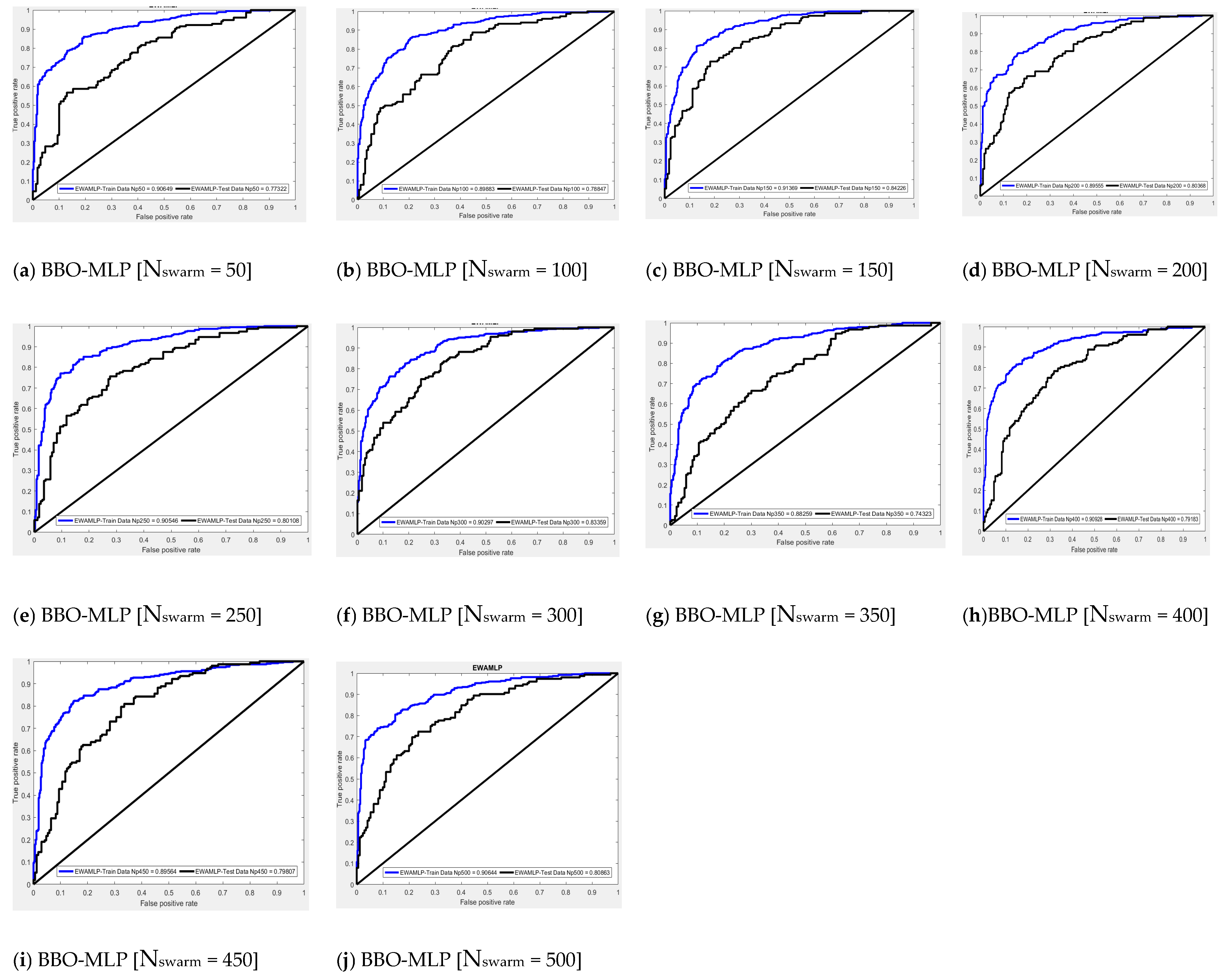
| Population Size | Network AUC Results | Scoring | Total Score | RANK | ||
|---|---|---|---|---|---|---|
| Training | Testing | Training | Testing | |||
| 50 | 0.906 | 0.773 | 8 | 2 | 10 | 6 |
| 100 | 0.899 | 0.788 | 4 | 3 | 7 | 9 |
| 150 | 0.914 | 0.842 | 10 | 10 | 20 | 1 |
| 200 | 0.896 | 0.804 | 2 | 7 | 9 | 7 |
| 250 | 0.905 | 0.801 | 6 | 6 | 12 | 5 |
| 300 | 0.903 | 0.834 | 5 | 9 | 14 | 3 |
| 350 | 0.883 | 0.743 | 1 | 1 | 2 | 10 |
| 400 | 0.909 | 0.792 | 9 | 4 | 13 | 4 |
| 450 | 0.896 | 0.798 | 3 | 5 | 8 | 8 |
| 500 | 0.906 | 0.809 | 7 | 8 | 15 | 2 |
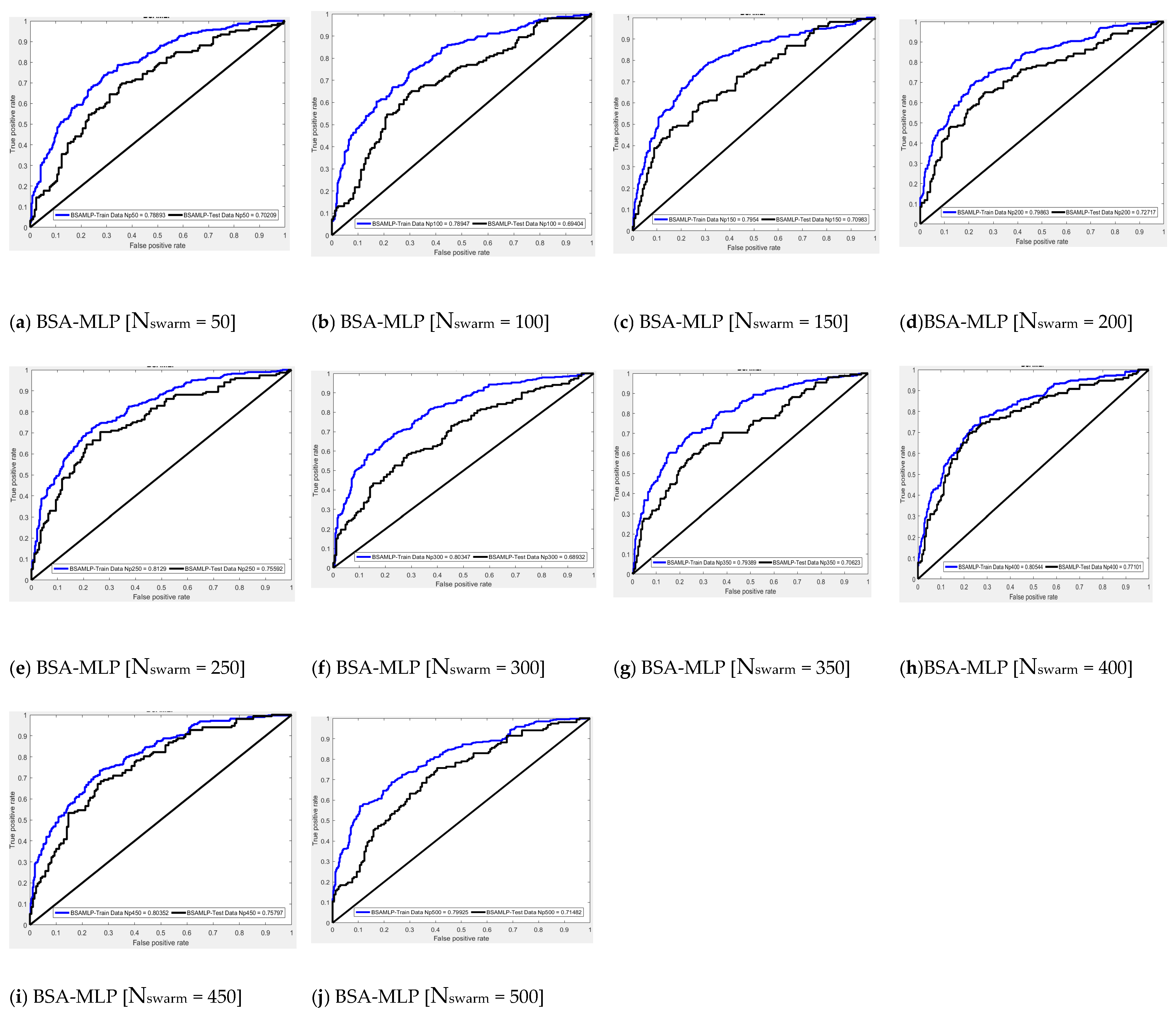
| Population Size | Network AUC Results | Scoring | Total Score | RANK | ||
|---|---|---|---|---|---|---|
| Training | Testing | Training | Testing | |||
| 50 | 0.789 | 0.702 | 1 | 3 | 4 | 9 |
| 100 | 0.789 | 0.694 | 2 | 2 | 4 | 9 |
| 150 | 0.795 | 0.710 | 4 | 5 | 9 | 6 |
| 200 | 0.799 | 0.727 | 5 | 7 | 12 | 4 |
| 250 | 0.813 | 0.756 | 10 | 8 | 18 | 2 |
| 300 | 0.803 | 0.689 | 7 | 1 | 8 | 7 |
| 350 | 0.794 | 0.706 | 3 | 4 | 7 | 8 |
| 400 | 0.805 | 0.771 | 9 | 10 | 19 | 1 |
| 450 | 0.804 | 0.758 | 8 | 9 | 17 | 3 |
| 500 | 0.799 | 0.715 | 6 | 6 | 12 | 4 |
Disclaimer/Publisher’s Note: The statements, opinions and data contained in all publications are solely those of the individual author(s) and contributor(s) and not of MDPI and/or the editor(s). MDPI and/or the editor(s) disclaim responsibility for any injury to people or property resulting from any ideas, methods, instructions or products referred to in the content. |
© 2023 by the authors. Licensee MDPI, Basel, Switzerland. This article is an open access article distributed under the terms and conditions of the Creative Commons Attribution (CC BY) license (https://creativecommons.org/licenses/by/4.0/).
Share and Cite
Moayedi, H.; Canatalay, P.J.; Ahmadi Dehrashid, A.; Cifci, M.A.; Salari, M.; Le, B.N. Multilayer Perceptron and Their Comparison with Two Nature-Inspired Hybrid Techniques of Biogeography-Based Optimization (BBO) and Backtracking Search Algorithm (BSA) for Assessment of Landslide Susceptibility. Land 2023, 12, 242. https://doi.org/10.3390/land12010242
Moayedi H, Canatalay PJ, Ahmadi Dehrashid A, Cifci MA, Salari M, Le BN. Multilayer Perceptron and Their Comparison with Two Nature-Inspired Hybrid Techniques of Biogeography-Based Optimization (BBO) and Backtracking Search Algorithm (BSA) for Assessment of Landslide Susceptibility. Land. 2023; 12(1):242. https://doi.org/10.3390/land12010242
Chicago/Turabian StyleMoayedi, Hossein, Peren Jerfi Canatalay, Atefeh Ahmadi Dehrashid, Mehmet Akif Cifci, Marjan Salari, and Binh Nguyen Le. 2023. "Multilayer Perceptron and Their Comparison with Two Nature-Inspired Hybrid Techniques of Biogeography-Based Optimization (BBO) and Backtracking Search Algorithm (BSA) for Assessment of Landslide Susceptibility" Land 12, no. 1: 242. https://doi.org/10.3390/land12010242