
Modeling on Urban Land Use Characteristics and Urban System of the Traditional Chinese Era (1930s) Based on the Historical Military Topographic Map

Abstract
:1. Introduction
2. Research Area, Data, and Methods
2.1. Definition of the Scope of the Research Area
2.2. Military Topographic Map Information
2.3. Ancient Chinese Administrative Divisions and Cities
2.4. Walled Cities in China
2.5. GIS Reconstruction
2.5.1. Reconstruction Process
2.5.2. Accuracy Evaluation
2.6. Fractal and Rank-Size Law
2.7. Coefficient of the Variation and the Urban Primacy Index
2.8. Space Lorentz Curve
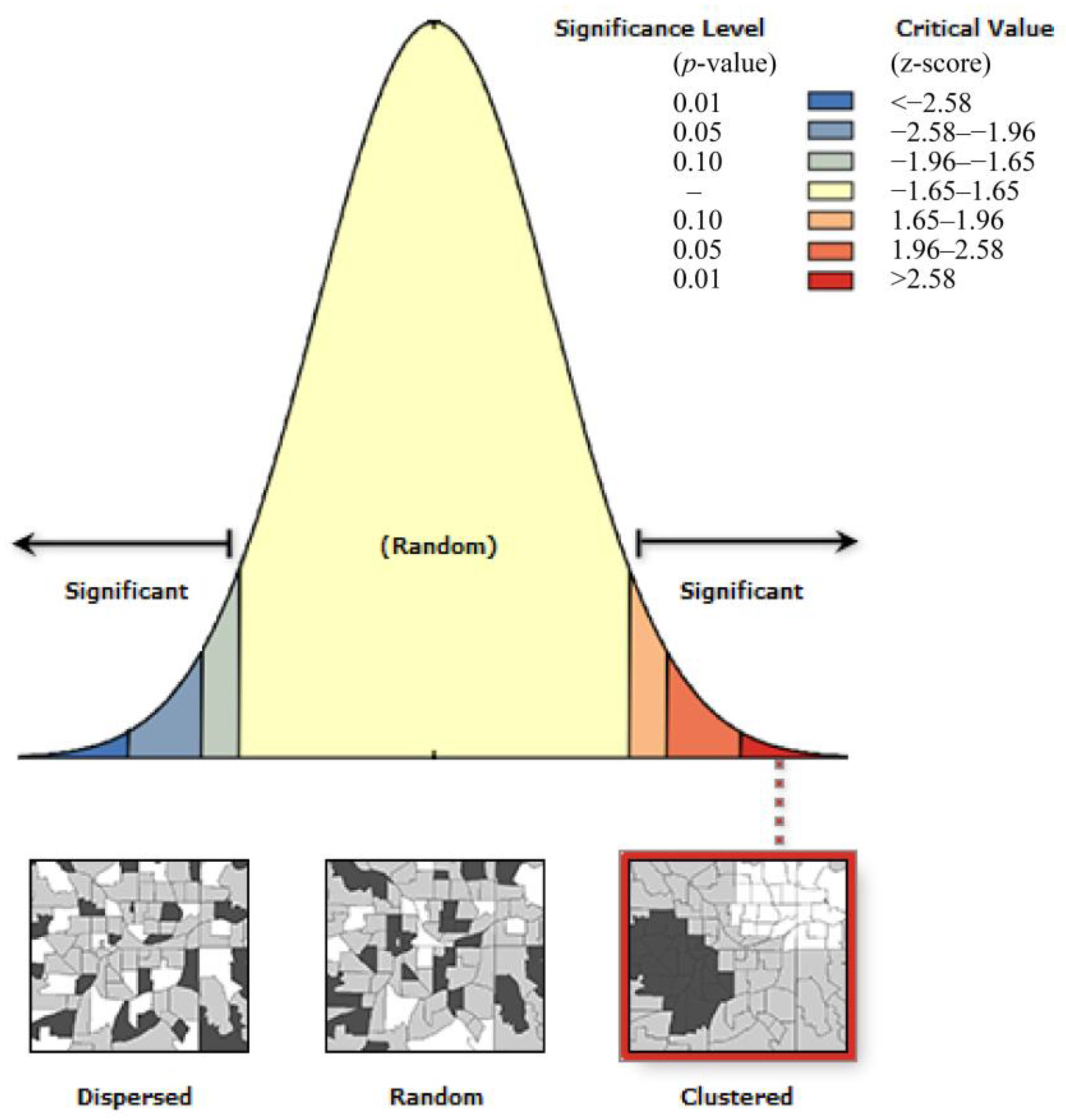
2.9. Getis–Ord Cold and Hotspot Analysis
3. Results
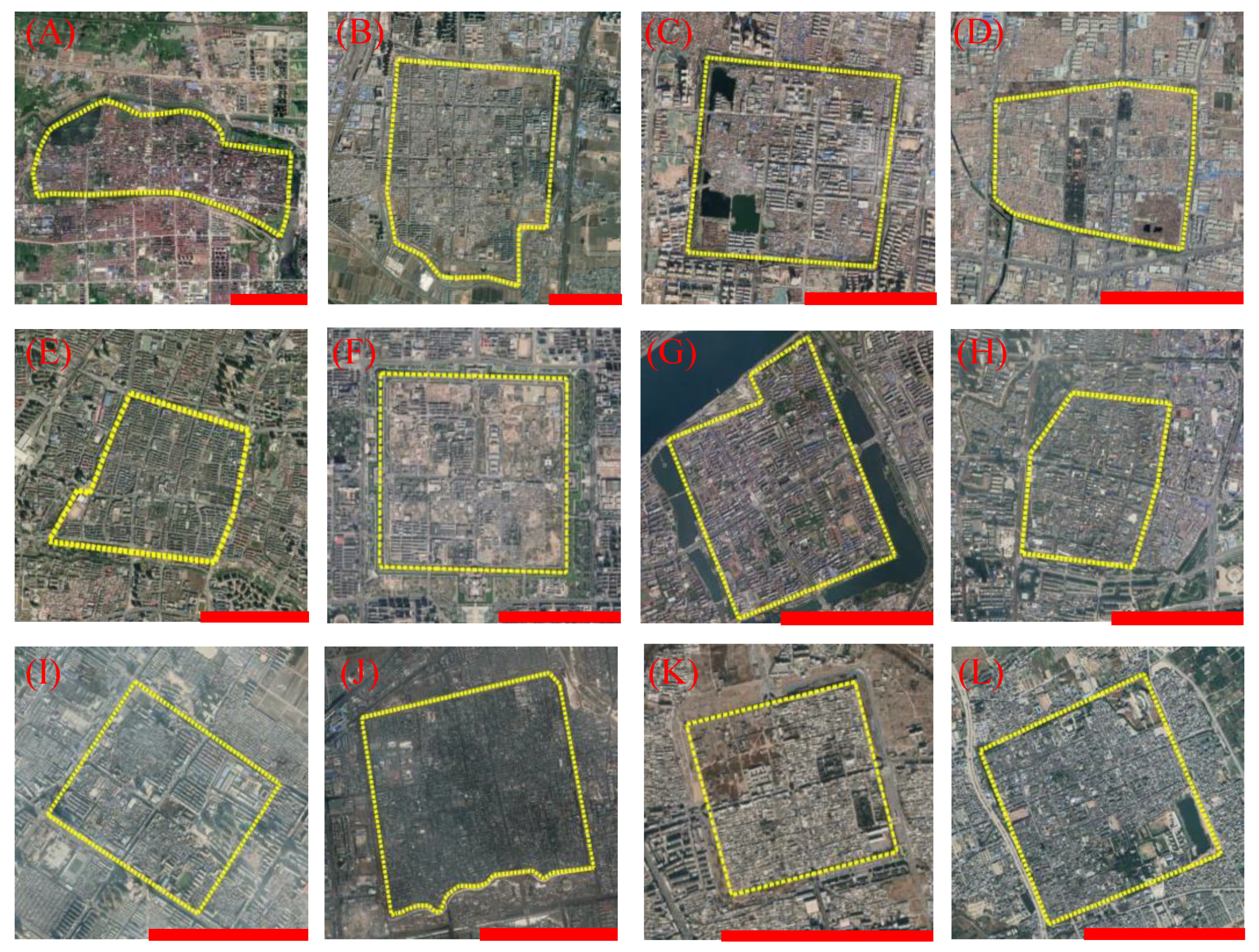
3.1. Urban Area Reconstruction
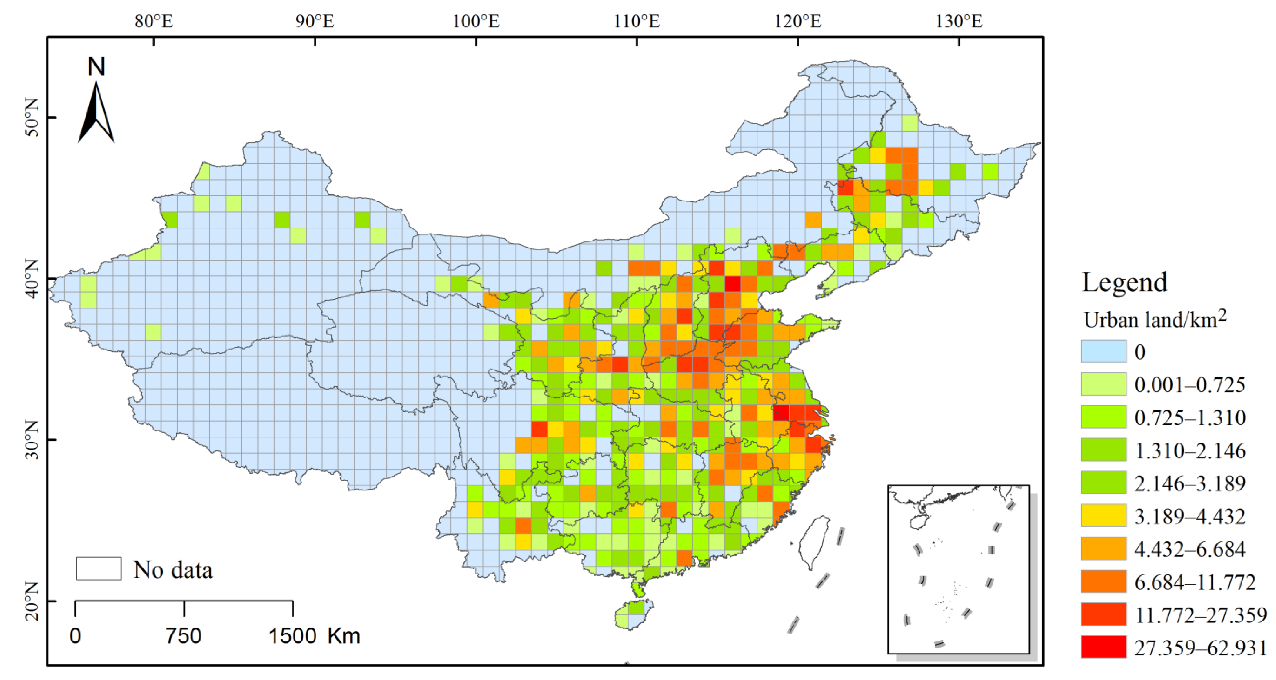
3.2. Level of Urbanization of the Grid
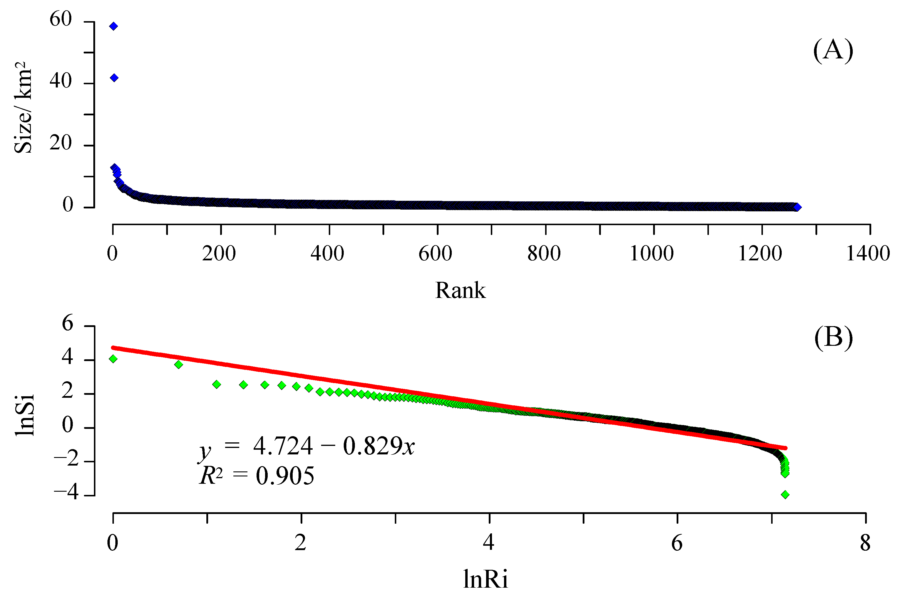
3.3. Urban System Structure
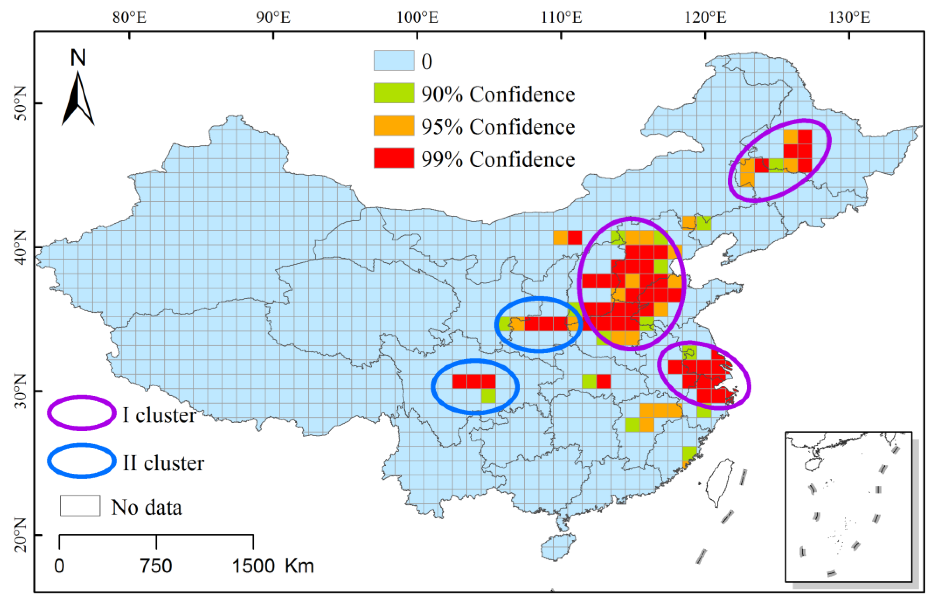
3.4. Spatial Clustering Characteristics
3.5. Spatial Trends
3.6. Characteristics of the Regional Agglomeration of Urbanization Levels
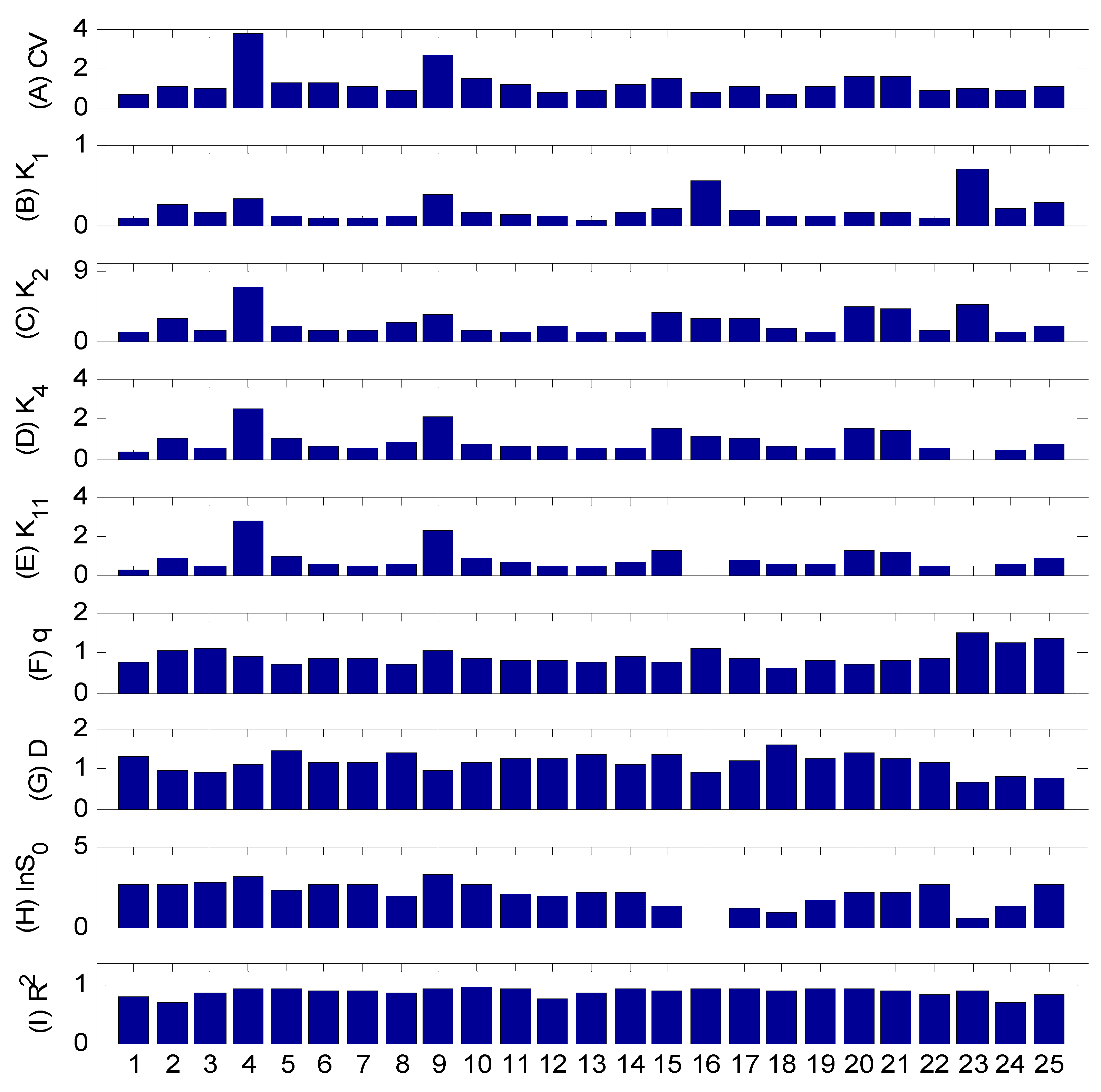
3.7. Differences in Urban Systems at the Provincial Level
4. Discussion
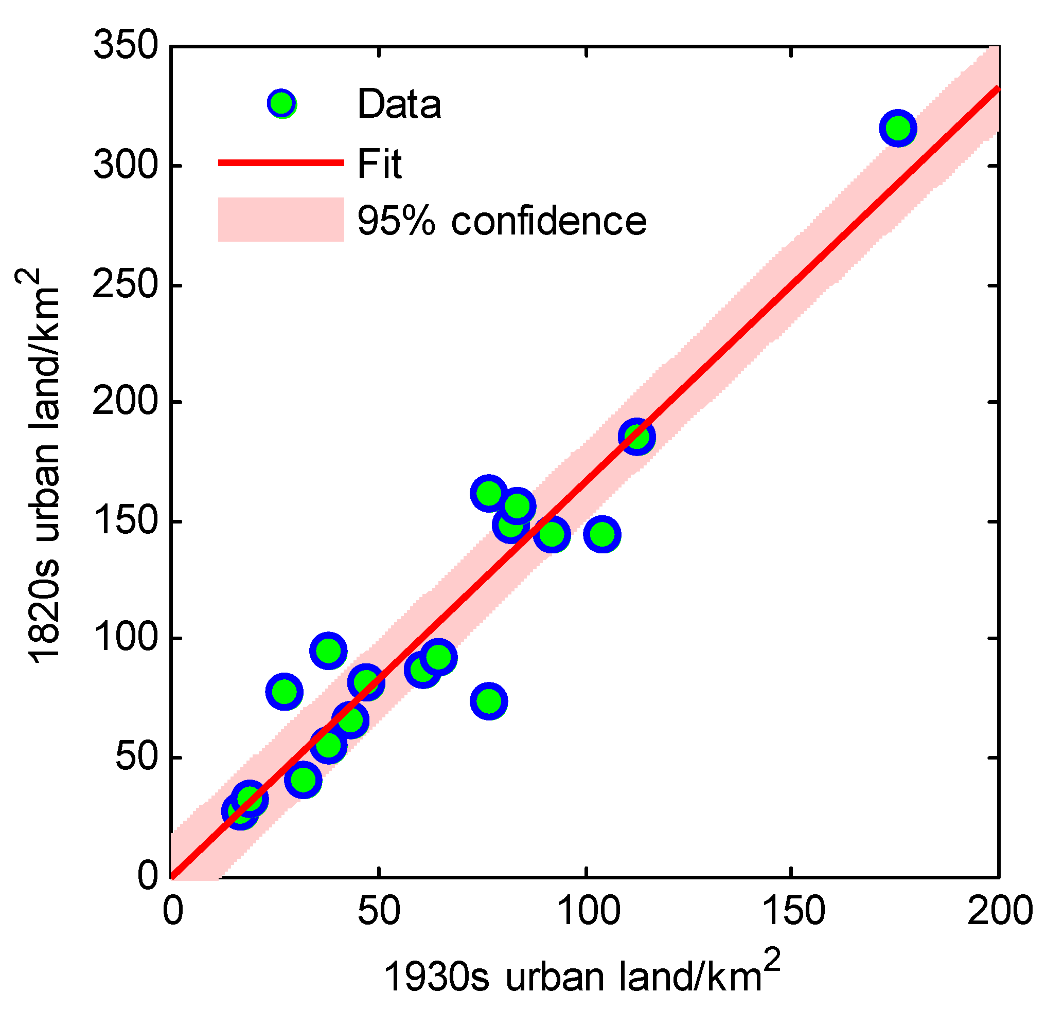
4.1. Comparison with Other Urban Land Use Data
4.2. Types of Urban Scale Systems
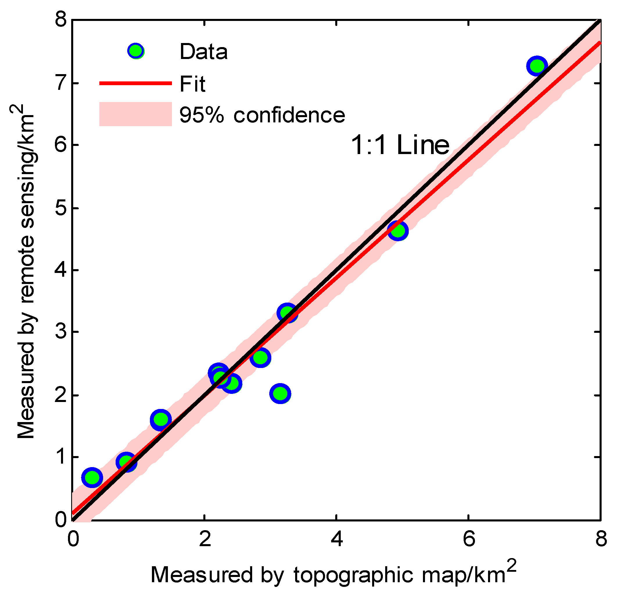
4.3. Uncertainty Analysis: A Comparison Using Remote Sensing Data
4.4. Limitations
5. Conclusions
- (1)
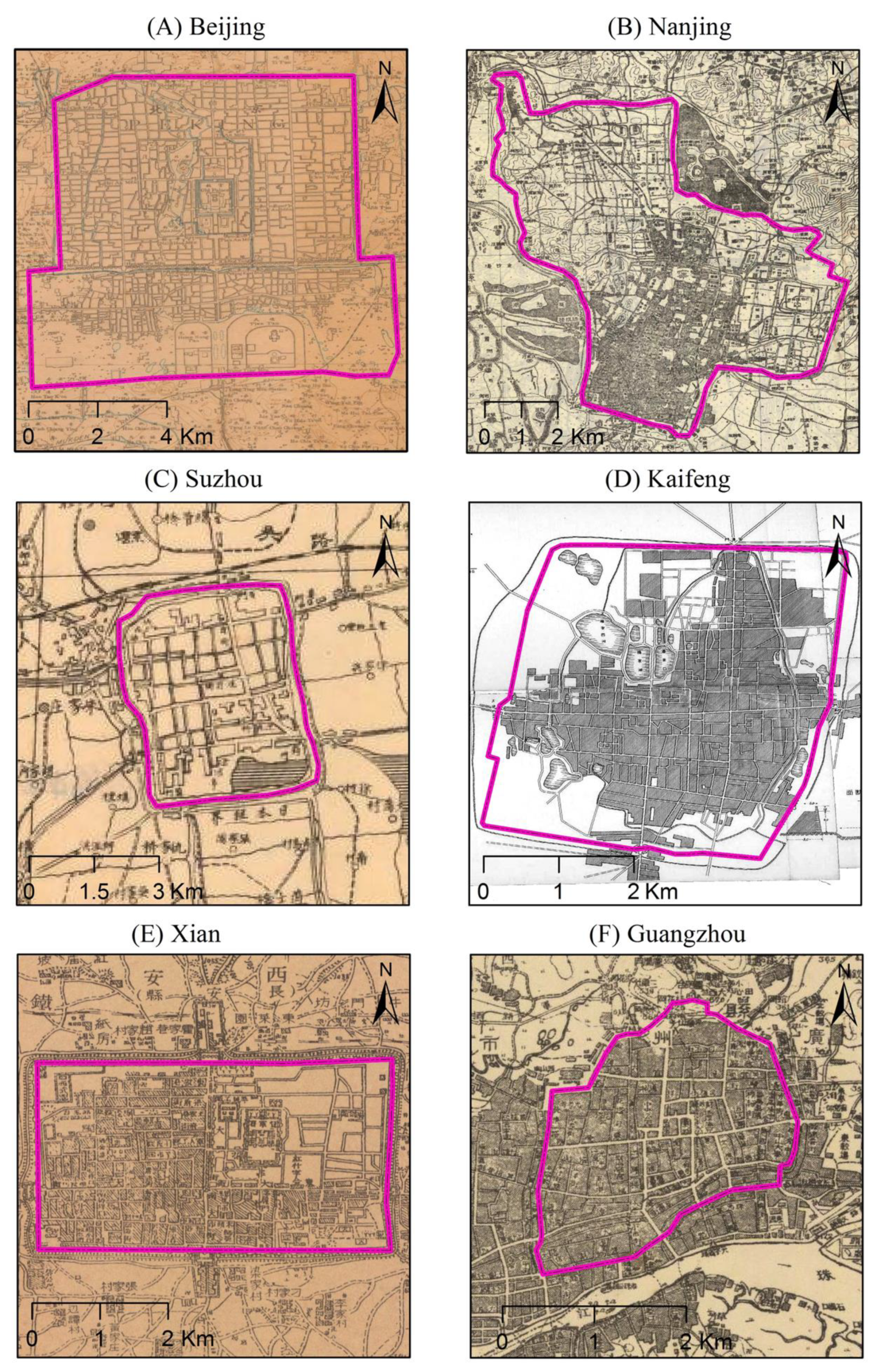
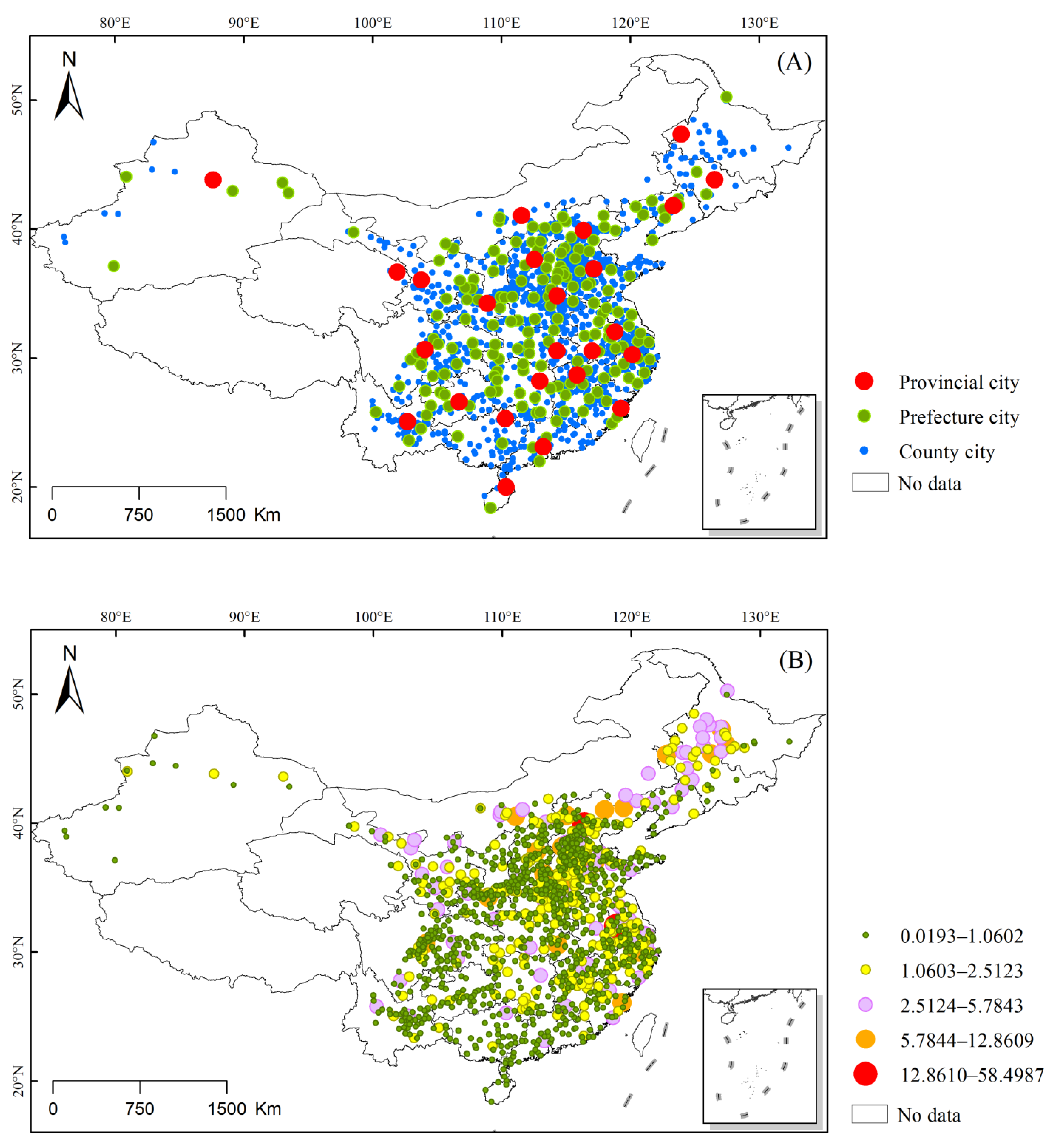
- A total of 1265 county level or above cities were counted in the TCE, including 25 provincial level or above cities, 179 prefectural level cities, and 1061 county level cities. Based on the extent of the city walls in TCE, the largest city was Beijing, with an area of 58.5 km2, and the smallest city was Jinghe in Xinjiang, with an area of 0.02 km2. The total land area of all of the cities was 1396.48 km2, with a mean value of 1.1 km2 and a standard deviation of 2.37 km2.
- (2)
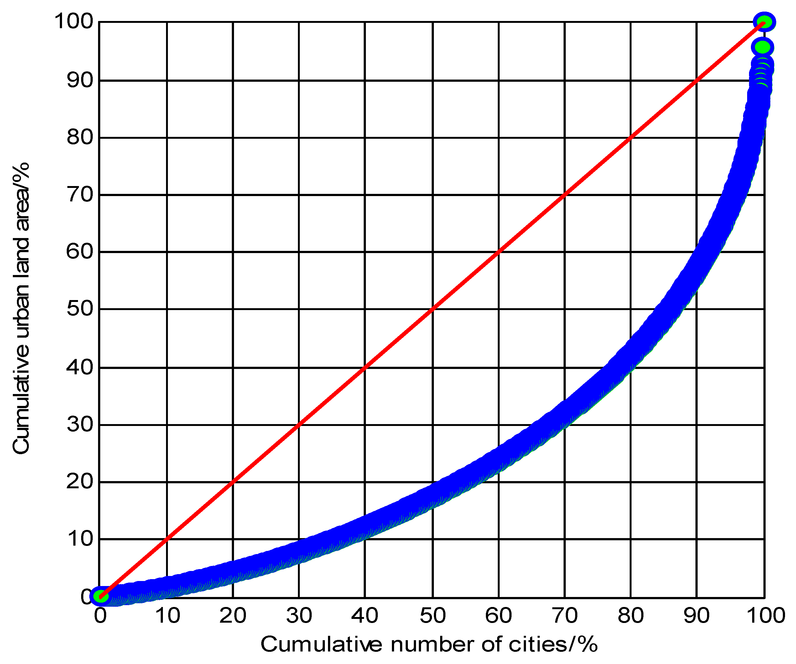
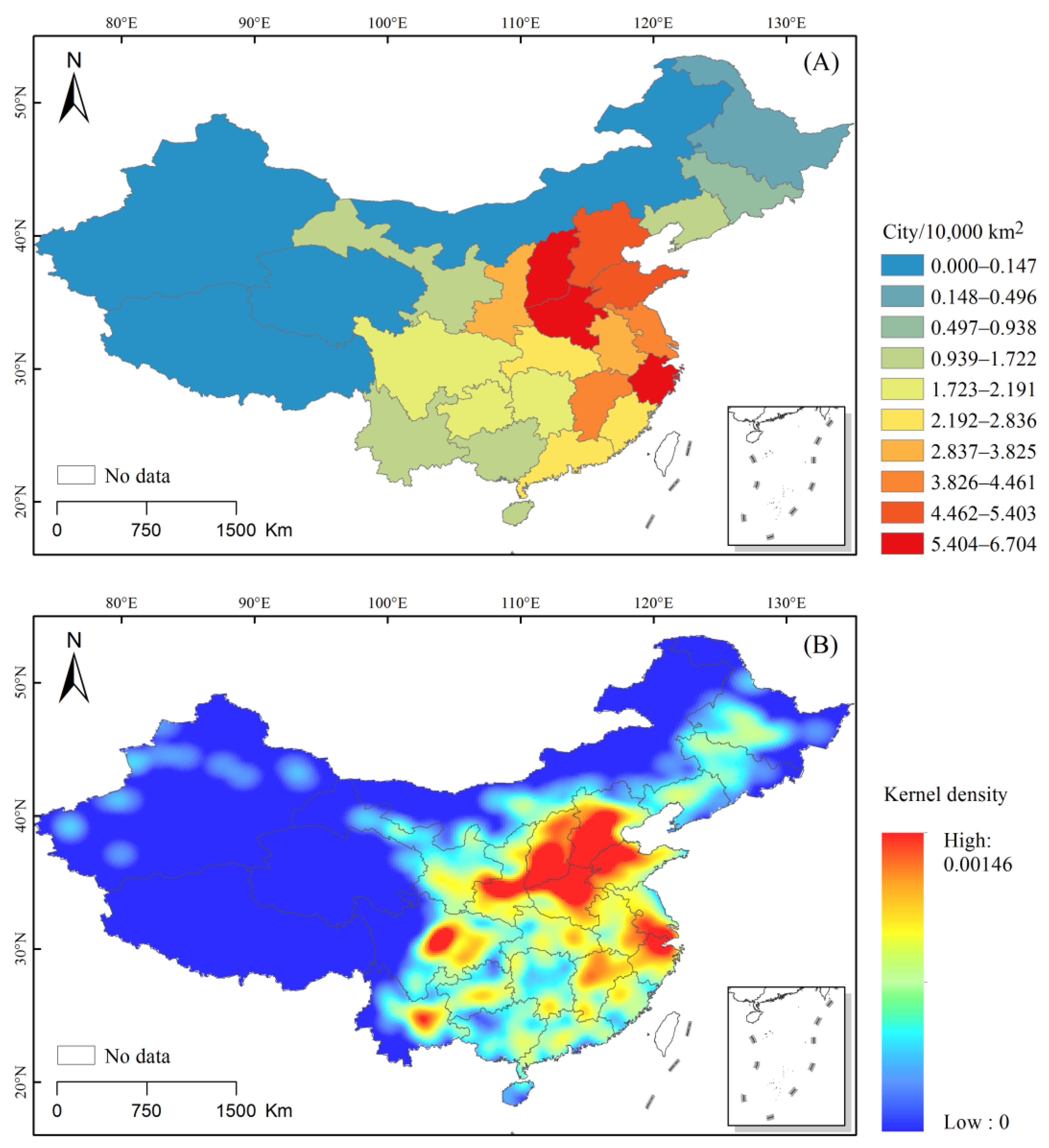
- The results of the rank-size analysis indicate that the urban system in the TCE was characterized by large cities with insignificant development (q = 0.829 < 1, R2 = 0.905) and a high proportion of county-level cities. The characteristics of this urban system were also related to the fact that in the 1930s, China was still a traditional agricultural country, the cities were more administrative-driven, and commercial cities had not yet developed. The results of the Lorenz curve and Moran analyses showed that the distribution of urban systems in China during the traditional period had a nonuniform spatial distribution of agglomeration.
- (3)
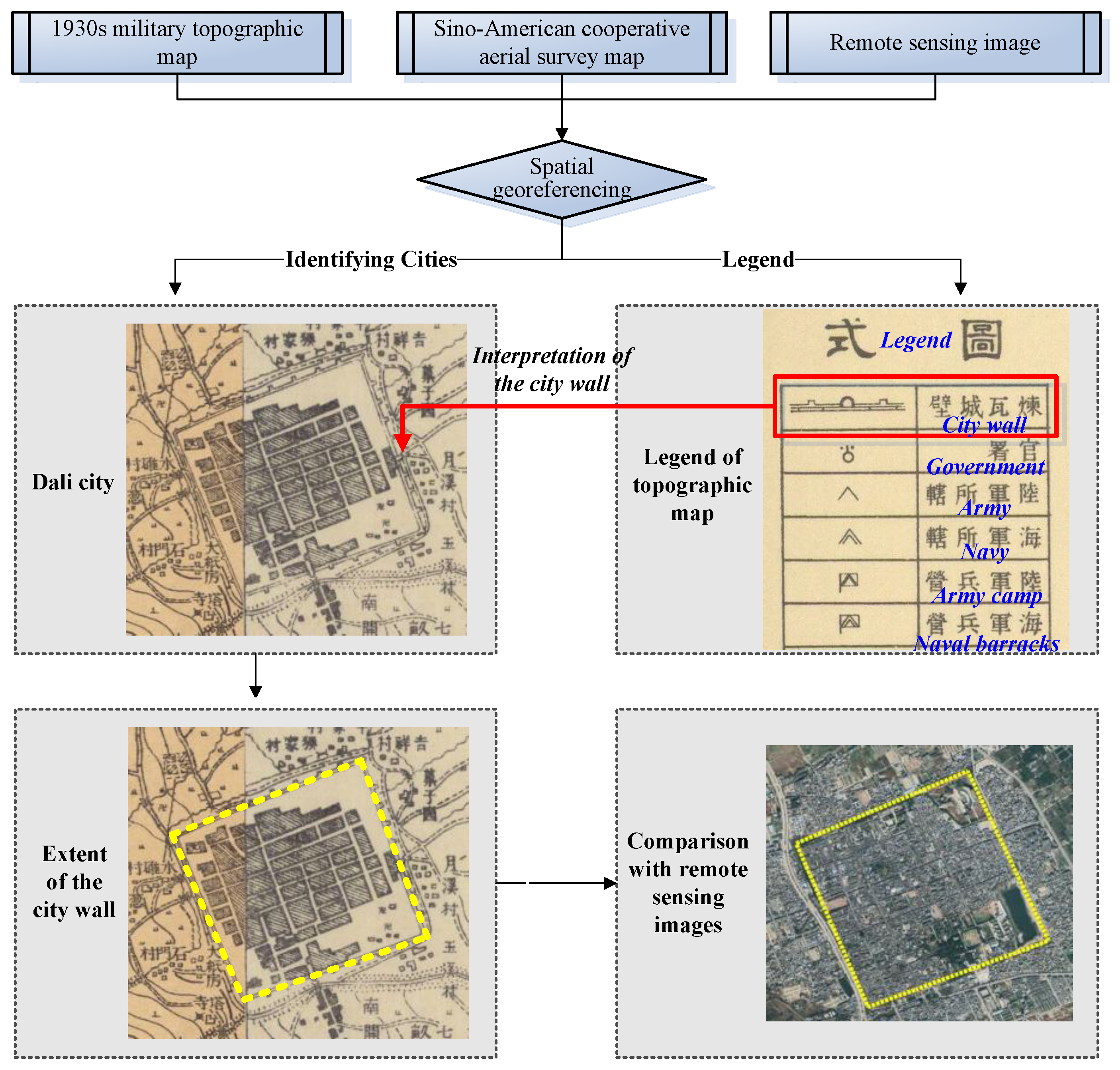
- Large-scale military topographic maps of historical periods have proven to be a good source for land use reconstruction. Uncertainty analysis showed that the military topographic maps for the 1930s have good accuracy, and the correlation coefficient between the reconstructed urban areas based on topographic maps and the area values obtained using remote sensing images was 0.976. The 1° × 1° gridded urban land area dataset constructed based on a GIS model of the TCE is important for future research on historical LUCC and can provide basic data for climate change models, urban economic history, and other disciplines.
Author Contributions
Funding
Institutional Review Board Statement
Informed Consent Statement
Data Availability Statement
Acknowledgments
Conflicts of Interest
References
- Proctor, J.D. The meaning of global environmental change: Retheorizing culture in human dimensions research. Glob. Environ. Chang. 1998, 8, 227–248. [Google Scholar] [CrossRef]
- Lambin, E.F.; Turner, B.L.; Geist, H.J.; Agbola, S.B.; Angelsen, A.; Bruce, J.W.; Coomes, O.T.; Dirzo, R.; Fischer, G.; Folke, C. The causes of land-use and land-cover change: Moving beyond the myths. Glob. Environ. Chang. 2001, 11, 261–269. [Google Scholar] [CrossRef]
- Houet, T.; Loveland, T.R.; Hubert-Moy, L.; Gaucherel, C.; Napton, D.; Barnes, C.A.; Sayler, K. Exploring subtle land use and land cover changes: A framework for future landscape studies. Landsc. Ecol. 2010, 25, 249–266. [Google Scholar] [CrossRef] [Green Version]
- Fu, C. Potential impacts of human-induced land cover change on East Asia monsoon. Glob. Planet. Chang. 2003, 37, 219–229. [Google Scholar] [CrossRef]
- Bae, J.; Ryu, Y. Land use and land cover changes explain spatial and temporal variations of the soil organic carbon stocks in a constructed urban park. Landsc. Urban Plan. 2015, 136, 57–67. [Google Scholar] [CrossRef]
- Mather, A.S.; Needle, C.L.; Fairbairn, J. The human drivers of global land cover change: The case of forests. Hydrol. Process. 1998, 12, 1983–1994. [Google Scholar] [CrossRef]
- Uhrqvist, O.; Lövbrand, E. Rendering global change problematic: The constitutive effects of Earth System research in the IGBP and the IHDP. Environ. Polit. 2014, 23, 339–356. [Google Scholar] [CrossRef]
- Brunn, S.D.; O’Lear, S.R. Research and communication in the invisible college of the Human Dimensions of Global Change. Glob. Environ. Chang. 1999, 9, 285–301. [Google Scholar] [CrossRef]
- Steffen, W. Introducing the Anthropocene: The human epoch. Ambio 2021, 50, 1784–1787. [Google Scholar] [CrossRef]
- Fang, X.; Zhao, W.; Zhang, C.; Zhang, D.; Wei, X.; Qiu, W.; Ye, Y. Methodology for credibility assessment of historical global LUCC datasets. Sci. China Earth Sci. 2020, 63, 1013–1025. [Google Scholar] [CrossRef]
- Alverson, K.; Oldfield, F. Pages: Past global changes and their significance for the future: An introduction. Quat. Sci. Rev. 2000, 19, 3–7. [Google Scholar] [CrossRef]
- Newman, L.; Kiefer, T.; Otto-Bliesner, B.; Wanner, H. The science and strategy of the Past Global Changes (PAGES) project. Curr. Opin. Environ. Sustain. 2010, 2, 193–201. [Google Scholar] [CrossRef]
- Morrison, K.D.; Tello, E.; Hammer, E.; Popova, L.; Madella, M.; Whitehouse, N.; Gaillard, M. Global-scale comparisons of human land use: Developing shared terminology for land-use practices for global change. Past Glob. Chang. Mag. 2018, 26, 8–9. [Google Scholar]
- Ioannides, Y.M.; Zhang, J. Walled cities in late imperial China. J. Urban Econ. 2017, 97, 71–88. [Google Scholar] [CrossRef] [Green Version]
- Ramankutty, N.; Foley, J.A. Characterizing patterns of global land use: An analysis of global croplands data. Glob. Biogeochem. Cycles 1998, 12, 667–685. [Google Scholar] [CrossRef]
- Ramankutty, N.; Foley, J.A. Estimating historical changes in global land cover: Croplands from 1700 to 1992. Glob. Biogeochem. Cycles 1999, 13, 997–1027. [Google Scholar] [CrossRef]
- Klein Goldewijk, K.; Beusen, A.; Van Drecht, G.; De Vos, M. The HYDE 3.1 spatially explicit database of human-induced global land-use change over the past 12,000 years. Glob. Ecol. Biogeogr. 2011, 20, 73–86. [Google Scholar] [CrossRef]
- Klein Goldewijk, K.; Beusen, A.; Janssen, P. Long-term dynamic modeling of global population and built-up area in a spatially explicit way: HYDE 3.1. Holocene 2010, 20, 565–573. [Google Scholar] [CrossRef] [Green Version]
- He, F.; Li, M.; Li, S. Reconstruction of Lu-level cropland areas in the Northern Song Dynasty (AD976-1078). J. Geogr. Sci. 2017, 27, 606–618. [Google Scholar] [CrossRef] [Green Version]
- Li, S.; He, F.; Zhang, X. A spatially explicit reconstruction of cropland cover in China from 1661 to 1996. Reg. Environ. Chang. 2016, 16, 417–428. [Google Scholar] [CrossRef]
- Liu, M.; Tian, H. China.s land cover and land use change from 1700 to 2005: Estimations from high-resolution satellite data and historical archives. Glob. Biogeochem. Cycles 2010, 24, 1–18. [Google Scholar] [CrossRef]
- Ge, Q.; Dai, J.; He, F.; Zheng, J.; Man, Z.; Zhao, Y. Spatiotemporal dynamics of reclamation and cultivation and its driving factors in parts of China during the last three centuries. Prog. Nat. Sci. 2004, 14, 605–613. [Google Scholar] [CrossRef]
- He, F.; Ge, Q.; Zheng, J. Reckoning the Areas of Urban Land Use and Their Comparison in the Qing Dynasty in China. Acta Geogr. Sin. 2002, 57, 709–716. [Google Scholar]
- He, F.; Li, S.; Zhang, X.; Ge, Q.; Dai, J. Comparisons of cropland area from multiple datasets over the past 300 years in the traditional cultivated region of China. J. Geogr. Sci. 2013, 23, 978–990. [Google Scholar] [CrossRef]
- Zheng, J.; Lin, S.; He, F. Recent progress in studies on land cover change and its regional climatic effects over China during historical times. Adv. Atmos. Sci. 2009, 26, 793–802. [Google Scholar] [CrossRef]
- Wan, Z.; Chen, X.; Ju, M.; Ling, C.; Liu, G.; Liao, F.; Jia, Y.; Jiang, M. Reconstruction and Pattern Analysis of Historical Urbanization of Pre-Modern China in the 1910s Using Topographic Maps and the GIS-ESDA Model: A Case Study in Zhejiang Province, China. Sustainability 2020, 12, 537. [Google Scholar] [CrossRef] [Green Version]
- Pan, W.; Man, Z. The grid methods of drainage density data reconstruction in big river delta: Based on the case of Qingpu, Shanghai, 1918-1978. J. Chin. Hist. Geogr. 2010, 25, 5–14. [Google Scholar]
- Chen, L.; Wang, Y. The profile of some military topographic map before 1949. Hubei Arch. 1999, 13, 31–32. [Google Scholar]
- Yang, X.; Jin, X.; Lin, Y.; Han, J.; Zhou, Y. Review on China’s spatially-explicit historical land cover datasets and reconstruction methods. Prog. Geogr. 2016, 35, 159–172. [Google Scholar]
- Jin, X.; Cao, X.; Du, X.; Yang, X.; Bai, Q.; Zhou, Y. Farmland dataset reconstruction and farmland change analysis in China during 1661-1985. J. Geogr. Sci. 2015, 25, 1058–1074. [Google Scholar] [CrossRef]
- Wan, Z.; Jia, Y.; Jiang, M.; Liu, Y.; Hong, Y.; Lu, C. Reconstruction of urban land use and urbanization level in Jiangxi Province during the Republic of China period. Acta Geogr. Sin. 2018, 73, 550–561. [Google Scholar]
- Jiang, W. The urban form of traditional mid-small cities: Focus on cadastral maps of Jurong county town in the Republic China. J. Chin. Hist. Geogr. 2014, 29, 33–45. [Google Scholar]
- Ren, Y.; Deng, F. Analysis of Cartographic Source Based on Map Integration of One in 50 000 in Mainland China. Chin. Hist. Geogr. 2020, 40, 132–142. [Google Scholar]
- Jiang, W. Number of Commercial Towns in Jiangnan:A Sharp Contrast of the Number of Commercial Towns between Changshu and Wujiang. J. Chin. Hist. Geogr. 2017, 32, 56–69. [Google Scholar]
- Zhou, Z. General History of China’s Administrative Divisions; Fudan University Press: Shanghai, China, 2007; pp. 1–785. [Google Scholar]
- Zhang, Y. History of Chinese Cities; Baihua Literature and Art Publishing House: Tianjin, China, 2003; pp. 1–605. [Google Scholar]
- Xie, J.; Jin, X.; Lin, Y.; Cheng, Y.; Yang, X.; Bai, Q.; Zhou, Y. Quantitative estimation and spatial reconstruction of urban and rural construction land in Jiangsu Province, 1820-1985. J. Geogr. Sci. 2017, 27, 1185–1208. [Google Scholar] [CrossRef]
- Cheng, Y. The Urban Size and Administrative Scales in the Qing Dynasty. J. Yangzhou Univ. 2007, 11, 124–128. [Google Scholar]
- Whitehand, J.; Gu, K. Urban conservation in China: Historical development, current practice and morphological approach. Town Plan. Rev. 2007, 78, 643–670. [Google Scholar] [CrossRef]
- Chen, Y. Modeling fractal structure of city-size distributions using correlation functions. PLoS ONE 2011, 6, e24791. [Google Scholar] [CrossRef] [Green Version]
- Chen, Y.; Zhou, Y. Multi-fractal measures of city-size distributions based on the three-parameter Zipf model. Chaos Solitons Fractals 2004, 22, 793–805. [Google Scholar] [CrossRef]
- Benguigui, L.; Czamanski, D. Simulation Analysis of the Fractality of Cities. Geogr. Anal. 2004, 36, 69–85. [Google Scholar] [CrossRef]
- Chen, Y.; Zhou, Y. The rank-size rule and fractal hierarchies of cities: Mathematical models and empirical analyses. Environ. Plan. B 2003, 30, 799–818. [Google Scholar] [CrossRef]
- Feng, J.; Chen, Y. Spatiotemporal evolution of urban form and land-use structure in Hangzhou, China: Evidence from fractals. Environ. Plan. B: Plan. Des. 2010, 37, 838–856. [Google Scholar] [CrossRef]
- Small, C. Global population distribution and urban land use in geophysical parameter space. Earth Interact 2004, 8, 1–18. [Google Scholar] [CrossRef]
- Li, N.; Wang, J.; Wang, H.; Fu, B.; Chen, J.; He, W. Impacts of land use change on ecosystem service value in Lijiang River Basin, China. Environ. Sci. Pollut. R. 2021, 28, 46100–46115. [Google Scholar] [CrossRef]
- Ord, J.K.; Getis, A. Local spatial autocorrelation statistics: Distributional issues and an application. Geogr. Anal. 1995, 27, 286–306. [Google Scholar] [CrossRef]
- Getis, A.; Ord, J.K. The analysis of spatial association by use of distance statistics. Geogr. Anal. 1992, 24, 189–206. [Google Scholar] [CrossRef]
- Xu, X.; Zhou, Y.; Ning, Y. Urban Geography; Higher Education Press: Beijing, China, 2009; pp. 1–355. [Google Scholar]


Disclaimer/Publisher’s Note: The statements, opinions and data contained in all publications are solely those of the individual author(s) and contributor(s) and not of MDPI and/or the editor(s). MDPI and/or the editor(s) disclaim responsibility for any injury to people or property resulting from any ideas, methods, instructions or products referred to in the content. |
© 2023 by the authors. Licensee MDPI, Basel, Switzerland. This article is an open access article distributed under the terms and conditions of the Creative Commons Attribution (CC BY) license (https://creativecommons.org/licenses/by/4.0/).
Share and Cite
Wan, Z.; Wu, H. Modeling on Urban Land Use Characteristics and Urban System of the Traditional Chinese Era (1930s) Based on the Historical Military Topographic Map. Land 2023, 12, 244. https://doi.org/10.3390/land12010244
Wan Z, Wu H. Modeling on Urban Land Use Characteristics and Urban System of the Traditional Chinese Era (1930s) Based on the Historical Military Topographic Map. Land. 2023; 12(1):244. https://doi.org/10.3390/land12010244
Chicago/Turabian StyleWan, Zhiwei, and Hongqi Wu. 2023. "Modeling on Urban Land Use Characteristics and Urban System of the Traditional Chinese Era (1930s) Based on the Historical Military Topographic Map" Land 12, no. 1: 244. https://doi.org/10.3390/land12010244