Article

Effects of Urban Form on Carbon Emissions in China: Implications for Low-Carbon Urban Planning

1
Department of Land Management, Zhejiang University, Hangzhou 310058, China
2
Key Laboratory of Urban Land Resources Monitoring and Simulation, Ministry of Natural Resources, Shenzhen 518034, China
*
Author to whom correspondence should be addressed.
Land 2022, 11(8), 1343; https://doi.org/10.3390/land11081343
Submission received: 21 July 2022 / Revised: 12 August 2022 / Accepted: 16 August 2022 / Published: 18 August 2022
(This article belongs to the Special Issue Urban Land Development in the Process of Urbanization)

Abstract

:
Carbon emissions are closely related to global warming. More than 70% of global carbon emissions have been generated in cities. Many studies have analyzed the effects of cities on carbon emissions, from the perspective of urbanization, economics, and land use, yet a detailed understanding of the relationship between urban form and carbon emissions is lacking due to the absence of a reasonable set of urban form metrics. The aim of this research is to explore the effects of urban form on carbon emissions through empirical research. By eliminating collinearity, we established a set of urban form landscape metrics comprising Class Area (CA), Mean Perimeter–Area Ratio (PARA-MN), Mean Proximity Index (PROX-MN), and Mean Euclidian Nearest Neighbor Distance (ENN-MN) representing urban area, complexity, compactness, and centrality, respectively. Through spatial autocorrelation analysis, the results show that there is a positive spatial autocorrelation of carbon emissions. The high–high agglomeration regions are located in the Beijing–Tianjin–Hebei and Yangtze River Delta, while the low–low agglomeration regions are concentrated in the Southwest and Heilongjiang Province. Based on a spatial error model, for the whole study area, CA, PARA-MN, and ENN-MN show a positive correlation with carbon emissions, but PROX-MN is the opposite. Based on ordinary least squares, PARA-MN in the Northeast and East, PROX-MN in the North and Mid-South, and ENN-MN in the North are significantly correlated with carbon emissions. These findings are helpful for low-carbon urban planning.

1. Introduction

Since the Industrial Revolution, coal, oil, natural gas and other forms of fossil energy have become the main resources for human life. The utilization of fossil energy leads to increased carbon emissions, causing global warming [1]. China is the largest developing country in the world. Its industrialization and urbanization have developed rapidly, and its carbon emissions are also increasing. In 2006, China surpassed the United States to become the country with the highest carbon emissions in the world [2]. In 2020, China’s carbon emissions accounted for 30% of global carbon emissions [3]. In the same year, China put forward the goals of peak carbon emissions in 2030 and carbon neutrality in 2060 [4,5].
As the center of human socio-economic activities, cities carry 85% of human production and economic activities [6], and generate more than 70% of global carbon emissions with 2% of the earth’s land area [7,8]. From 1990 to 2018, China’s urban population and construction land area grew significantly [9]. On the one hand, the rapid development of cities has expanded the scale of production activities and increased the consumption of fossil energy. On the other hand, the outward expansion of urban area continues to encroach on farmland and forests, resulting in a reduction in carbon sinks. In fact, as much as 50% of carbon emissions in cities are attributed to the choice of urban form [10]. For example, the increase in carbon emissions is affected by the intensity effect, expansion effect and economic effect to different degrees [8]. Urban form affects residents’ carbon emissions mainly through the housing market, losses in power transmission and the urban heat island effect [11]. Furthermore, urban form affects regional meteorological factors. For instance, urban form can influence the urban heat island effect through energy consumption, ultimately increasing carbon emissions [12]. In addition, carbon reduction, a priority for future development, requires an important foundation that can consolidate its achievements in order to achieve its sustainability. The urban form, as the physical foundation of cities, is relatively stable. It is also spatially integrated and interacts with economic and demographic factors, ultimately leading to a long-term effect of urban form on carbon emissions [13]. Thus, the urban form is not only an important factor in reducing carbon emissions but also an important vehicle for sustaining low-carbon sustainable development in the future. Exploring the effects of urban form on carbon emissions could provide a new perspective to achieve low-carbon sustainable development.
Due to the different connotations of urban form, there are many types of urban form measurement metrics. The first category is dominated by socio-economic metrics, including urbanization [14], economy [15], land use [13,16] and climate [5]. First, urbanization is an important metric affecting carbon emissions. In the early stage of urbanization, urban carbon emissions efficiency decreases with the growth of urban areas and their populations, but as the level of urbanization exceeds a certain point, carbon emissions efficiency increases instead. The impact of urbanization on carbon emissions shows a U-shaped trend [15]. Currently, the urbanization of Chinese cities shows large regional differences, with some cities growing while others are shrinking [4]. However, in general, China’s level of urbanization is in the first half of a U-shaped line, with the huge pressures of population growth and the environment. Thus, urbanization shows a positive relationship with carbon emissions [17]. Second, different industrial distributions and structures can change the effects of the economy on carbon emissions. Therefore, a large number of studies have classified economic data. For example, per capita GDP [18], industrial SO2 emissions per capita and the proportion of employees in the secondary sector are positively related to carbon emissions, while the proportion of employees in the three sectors and population density are negatively related to carbon emissions [19]. Third, influenced by urban density, community layout and building heights [20,21], specific land-use types can generate more carbon emissions. Retail trade and residential land have larger carbon emissions, while terrace houses produce more carbon emissions than other residential building categories [16]. Finally, climate shows a negative effect on carbon emissions [22]. This trend is mainly from the increase in temperature and precipitation [5]. Increased temperatures usually directly enhance autotrophic and heterotrophic soil respiration, and the increased precipitation can intensify soil erosion and lead to losses in soil nutrients, ultimately affecting ecosystem productivity and carbon sink functions. The second category of urban form measurement metrics is mainly based on the geometric characteristics of urban forms. Measures of the geometric characteristics are constantly changing as cities grow. In the early urbanization process, the population moved from rural to urban area, so urban areas became the most direct indicator of urban form [23]. With the expansion of cities, the ability of single-dimensional metrics to explain them is decreasing, and high-density land use is becoming the future direction of urban planning. Metrics such as compactness, complexity and centrality have been incorporated into the measurement dimensions of urban form. Compact development is associated with a high density of urban areas. The reduced distances between urban parts can reduce the need for transport and tourism, which directly reduces carbon emissions [24]. Complexity refers to the roughness of the urban patch perimeter. It has been proven that there is a positive correlation between complexity and carbon emissions [25]. Since landscape metrics can combine the characteristics of patch size, shape and quantity, they play an important role in the study of the spatiotemporal characteristics of urban land use [26] and the prediction of future morphological changes [27].
Since different urban forms have different effects on carbon emissions [
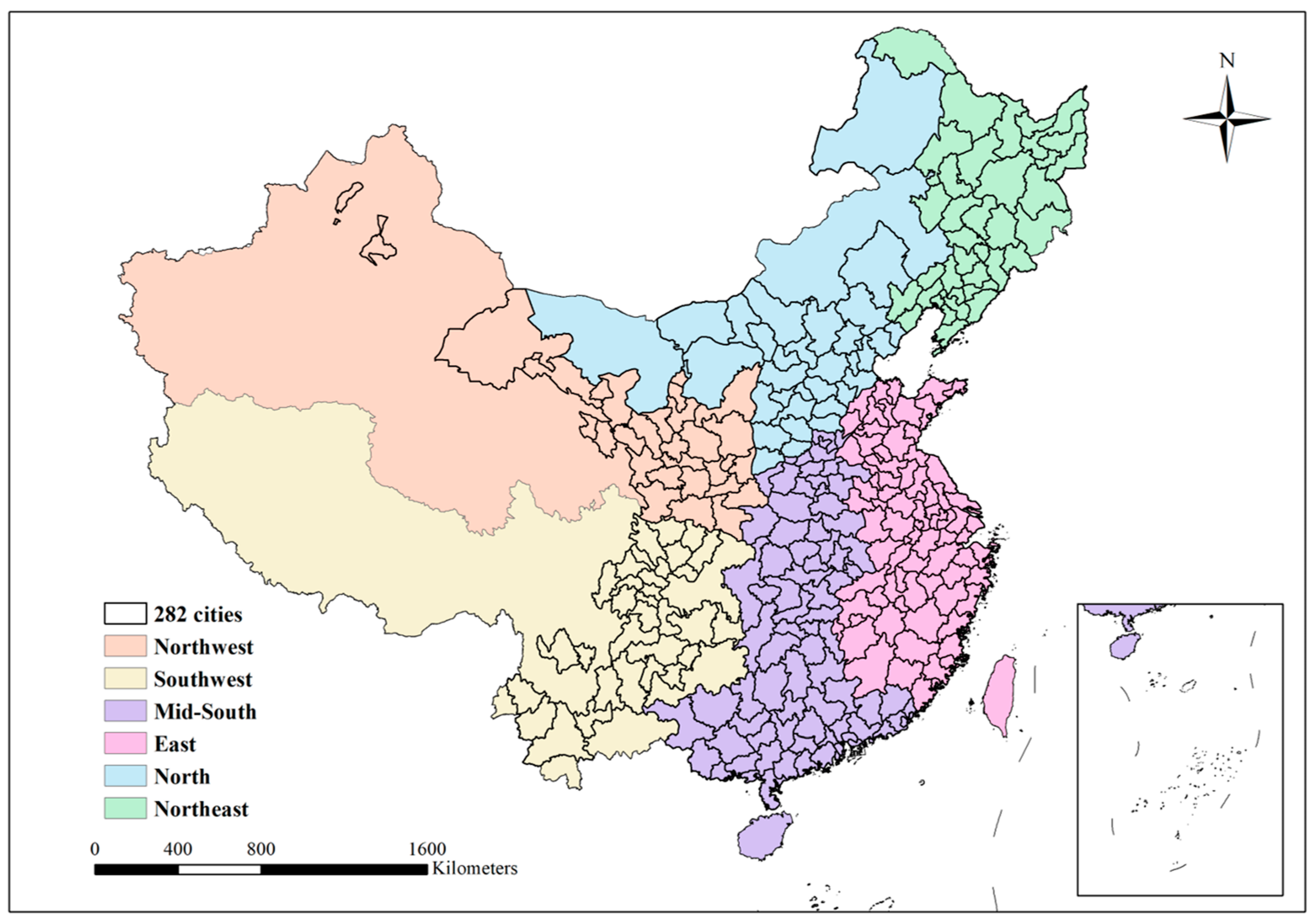
28], it is important to analyze their relationship from an appropriate perspective. Although some studies have begun to focus on the relationship between landscape metrics and carbon emissions, most of them considered landscape metrics as a driving factor, and integrated them with other factors such as urbanization and economy in one metric set. However, the urban form landscape metric includes multiple subdivision concepts such as urban area, compactness and centrality, which can not only directly reflect the level of urbanization, but also reflect the economic development and policy orientation of the region. Considering the rich information of landscape metrics, we need to select appropriate metrics from a large number of landscape metrics for analyzing their effects on carbon emissions. Therefore, the following hypotheses are proposed: urban form landscape metrics affect carbon emissions, and the effect of each metric changes from region to region. In order to prove these hypotheses, this study selected 282 cities at the prefectural level and above in China as an example. The aim of the presented research was to construct a reasonable set of urban form metrics through stepwise linear regression, analyze the effects of the urban form on carbon emissions through the spatial error model and ordinary least squares, and propose relevant policy recommendations for low-carbon urban planning.
In detail, there are two main contributions of this study. On the one hand, a set of reasonable urban form landscape metrics was constructed by stepwise linear regression This metric set can help in the selection of metrics for future research. On the other hand, key urban form metrics, which are significantly associated with carbon emissions in each region, are found, providing a reference for empirical research on the effects of urban form on carbon emissions and helping to suggest targeted improvements for low-carbon city planning. The rest of this paper is organized as follows: the Section 2 includes the study area and data; the Section 3 presents the methods; the Section 4 contains the results and discussion; and the Section 5 provides conclusions.

2. Study Area and Data

2.1. Study Area

Due to the lack of carbon emission data in the Tibet Autonomous Region, Hong Kong, Macau and Taiwan, 282 cities at the prefectural level and above in China were selected as the study area. Because of the vast size of China, carbon emissions vary greatly from region to region. In order to explore the impact of different urban forms on carbon emissions and provide more policy recommendations for low-carbon urban planning, cities need to be classified. This study classifies China’s administrative regions according to traditional geographic locations. It has been proven that the geographical location of cities and regional policies affects the urban form [29]. The traditional geographical divisions divide China into six regions, which are the North, Northeast, East, Mid-South, Southwest, and Northwest [30]. This method can analyze the driving factors affecting carbon emissions and provide more specific suggestions. Figure 1 shows the classification results of the 282 cities, comprising 30 cities in the Northwest, 33 cities in the Southwest, 77 cities in the Mid-South, 76 cities in the East, 34 cities in the Northeast and 32 cities in the North.

2.2. Data

There are mainly carbon emissions and urban form data in this study. The carbon emissions data were obtained from the carbon emissions inventory at the county level in China developed by Chen et al. [31] (https://www.ceads.net.cn/data/county/ (accessed on 1 April 2022)). This inventory is based on nighttime light data and uses the particle swarm optimization back-propagation (PSO-BP) algorithm to downscale the energy carbon emissions of each province. Finally, the carbon emissions of 2735 county-level energy sources from 1997 to 2017 were calculated. We summarized the county-level to city-level carbon emissions, and those of the 282 cities were obtained.
Urban form landscape metrics are based on the urban built-up area. Impervious surface data, as a typical representative of urban built-up areas, can be used directly in the calculation of urban form [32]. The national 40-year urban impervious surface data released by Gong et al. [33] (http://data.ess.tsinghua.edu.cn (accessed on 1 April 2022)) was used as the basic remote sensing data source for calculating urban form metrics. This dataset comprehensively considers MODIS and nighttime light data, classifies urban and rural impervious surfaces, and finally derives the annual dynamic change data of impervious surfaces within the urban area from 1978 to 2017. In order to improve the efficiency of data, the spatial resolution of the impervious surface data in 2017 was resampled to 100 m. Then, the urban administrative map was used for cropping to obtain the impervious surface distribution map of 282 cities in 2017.

2.3. Urban Form Landscape Metrics

In terms of urban area, patchiness, urban irregularity and urban compactness [28,34,35,36], 15 urban form landscape metrics were selected. We divided them into four categories: area, edge, shape and aggregation. (The equations and specific descriptions of the 15 metrics are shown in Table A1 in Appendix A).
For the metric of area, Class Area (CA) represents the total area of all urban patches. The Number of Patches (NP) can measure the urban fragmentation. The Largest Patch Index (LPI) is equal to the percentage of the total landscape area occupied by the largest urban patch.
For the indicator of edge, Edge Density (ED) is the sum of the lengths of all edge segments divided by the total landscape area.
For the metric of shape, the Area-weighted Mean Shape Index (AWMSI) at the patch level is equal to the sum of the perimeter-to-area ratio of each urban patch multiplied by the proportion of the entire urban patch area to the landscape area. Based on the AWMSI formula, the Area-weighted Mean Patch Fractal Dimension (AWMPFD) introduces a fractal dimension to weight all patches. However, the fractal dimension depends on the patch size and the units used. Therefore, changing the cell size of the input image will affect the AWMPFD to a large extent. Mean Perimeter–Area Ratio (PARA-MN) is the ratio of the total perimeter of urban patches to the total area of the area.
For the indicator of aggregation, the Landscape Shape Index (LSI) measures the perimeter–area ratio of urban patches. The Clumpiness Index (CLUMPY) reflects the degree of aggregation between urban patches. The Percentage of Like Adjacencies (PLADJ) represents the degree of connectivity within the urban built-up area. The Patch Cohesion Index (COHESION) is the ratio of the area-weighted average perimeter–area ratio to the area-weighted average patch shape index. Its formula is similar to PARA, but the interpretation of changes is more robust. The Aggregation Index (AI) examines the connectivity between patches of each landscape type. Patch Density (PD) represents the urban patch area per unit area. The Mean Proximity Index (PROX-MN) refers to the sum of the ratios of the size of all urban patches to the edge-to-edge distances of their nearest neighbors within a specified search radius. The Euclidian Mean Nearest Neighbor Distance (ENN-MN) quantifies the average distance between the two closest urban patches.
Based on the impervious surface distribution in 282 cities in 2017, the above 15 urban form landscape metrics were calculated. To eliminate the effect of differences in data magnitude, we normalized all variables by extreme value normalization, and the equation is as follows:
X = x x m i n x m a x x m i n

3. Methods

Highly correlated metrics could lead to redundant information, so it is necessary to judge whether there is multicollinearity by analyzing the variance inflation factors (VIF) of the metrics. Stepwise linear regression was used to eliminate the multicollinearity of metrics. Then, to investigate the effects of the urban form on carbon emissions, spatial autocorrelation analysis was applied to determine the spatial dependence of carbon emissions. Finally, the spatial error model and ordinary least squares were used to analyze the effect of each urban form metric on carbon emissions.

3.1. Stepwise Linear Regression

Stepwise linear regression is one of the most common methods of eliminating multicollinearity in variables. Its basic principle is to select the most important variables from a large number of variables. We used forward stepwise linear regression [37], adding one variable at a time until there were no new significant variables. The variables were introduced on the condition that they were statistically significant (p < 0.1) and to avoid multicollinearity (VIF < 10).

3.2. Spatial Autocorrelation Test

Only if there is a spatial dependence on carbon emissions can the spatial regression method be used. The spatial autocorrelation is used to test spatial dependence, including global spatial autocorrelation and local spatial autocorrelation [38]. Moran’s I is the most popular indicator to explore spatial autocorrelation. The calculation formula is as follows:
Moran s   I = i = 1 n j = 1 n ω i j ( CE i CE ¯ ) ( CE j CE ¯ ) S 2 i = 1 n j = 1 n ω i j
where n is the total number of cities; CEi and CEj represent the carbon emissions of city i and j, respectively; ωij represents the spatial weight; CE ¯ is the mean carbon emissions and S2 is the sample variance. Moran’s I has a value between −1 and 1. If the value exceeds 0, it means that there is a positive spatial autocorrelation of carbon emissions; conversely, it means that there is a negative spatial autocorrelation. If the value is close to 0, it means that there is no spatial independence.

3.3. Spatial Error Model

The spatial error model (SEM) is used to quantify the effects of the urban form on carbon emissions (for the choice of SEM, please see Appendix B). The SEM is different from the ordinary linear regression model, because its dependent variable is influenced not only by the independent variables in the region, but also by the independent variables in the neighboring regions. The SEM is expressed as follows [39]:
C E = β X + λ W μ + ε ,   ε   ~   N   [ 0 ,   δ 2 I n ] ,
where β is a coefficient vector, X is a matrix of the independent variables, λ is the spatial error factor, Wμ is the spatial weight matrix and ε is the stochastic error.

3.4. Ordinary Least Squares

If there is no spatial dependence on carbon emissions in the spatial autocorrelation test, or if carbon emissions and the urban form do not pass the Lagrange Multiplier test, then the next step is to use ordinary least squares (OLS) for multiple regression analysis. The OLS is expressed as follows:
C E = α + β X + ε
where α is the regression constant, β is the regression coefficient, X is the independent variable and ε is the stochastic error.

4. Results and Discussion

4.1. Urban Form Metrics Set

The results of the multicollinearity test for the metrics are shown in Table 1. The VIF values of 10 metrics, comprising CA, NP, ED, AWMSI, AWMPFD, LSI, CLUMPY, PLADJ, AI and PD, are higher than 20, indicating that these metrics contain redundant information and ordinary linear regression is inappropriate. In the stepwise linear regression, the independent variables comprise 15 landscape metrics, and the dependent variable is carbon emissions. The results are shown in Table 2. The final five metrics remaining in the model are CA, PARA-MN, PROX-MN, ENN-MN and PLADJ. The R2 of the model is 0.739, and the model passes the F-test (F = 155.968, p < 0.05).
Each VIF of the metric remaining in the stepwise linear regression model is less than 5, and the multicollinearity problem is statistically solved. However, due to the potential overlap between the metrics descriptions, we needed to optimize the metric set. First, CA, PARA-MN and ENN-MN depict different contents, but CLUMPY and PROX-MN both depict urban compactness. Second, CLUMPY requires patches to be adjacent. However, PROX-MN considers the size and proximity of all patches within the specified search radius of the edge, and there is no requirement that there must be a neighboring relationship between urban patches. Thus, we eliminated CLUMPY. Finally, the set of urban form metrics included the four metrics of CA, PARA-MN, PROX-MN and ENN-MN.

4.2. Analysis of Landscape Metrics and Carbon Emissions

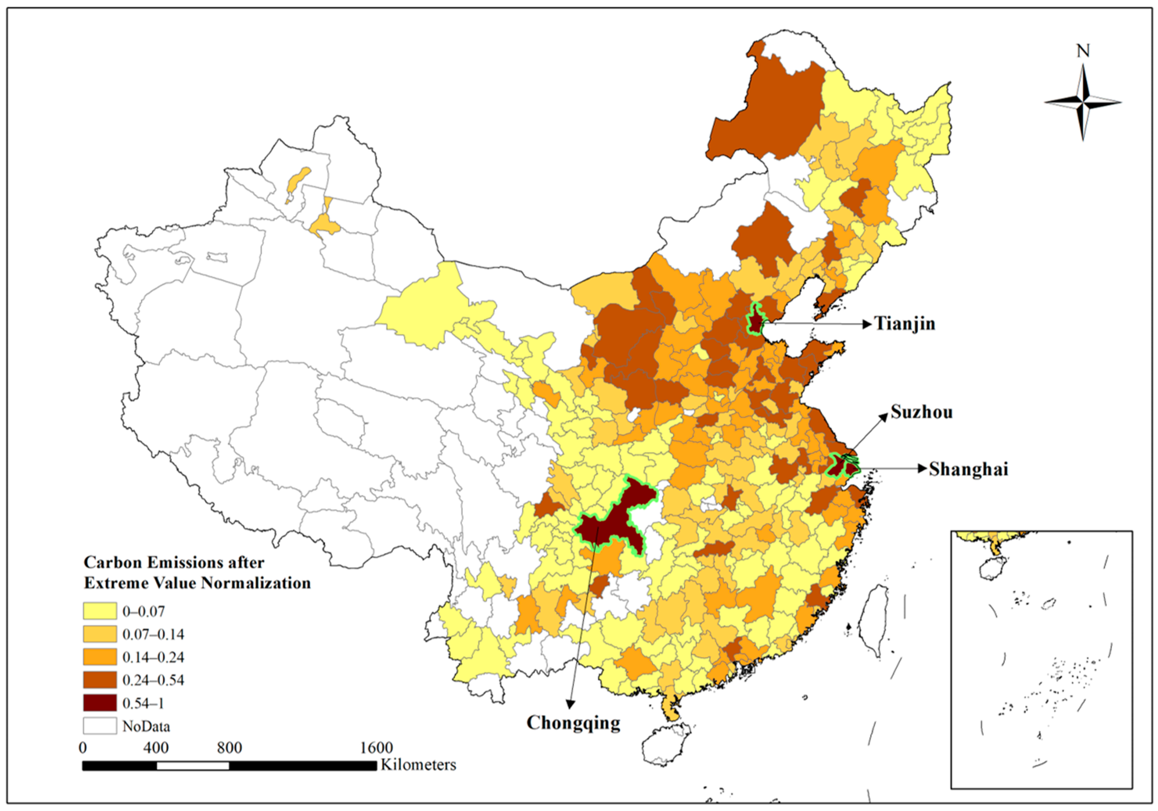
The results for the 282 cities’ carbon emissions after extreme value normalization in 2017 are shown in Figure 2. Shanghai, Chongqing, Tianjin and Suzhou are the four cities with the highest grade. The high-carbon-emissions cities are mainly distributed in the North and East, and are concentrated in Henan, Jiangsu, Hebei, Shandong, Shanxi and Zhejiang Province.
The carbon emissions and landscape metrics statistics of the study area are shown in Table 3. The characteristics of each region are as follows.
First, the average carbon emissions of the Norther region are nearly twice the national average, making it a high-carbon-emitting region. Influenced by carbon outflows from Beijing, Tianjin and other central cities, the North region contains more high-carbon-emissions cities than any other region. These central cities gather a large amount of resources, but the carbon emissions generated by its production resources are burdened by neighboring cities [40]. For example, urban-household-embedded carbon emissions in Shanxi, Hebei and Henan provinces increased from 37 Mt in 2002 to 97 Mt in 2012, while that for Beijing and Tianjin only increased from 9 Mt to 21 Mt [41]. The CA and PROX-MN of the cities in the North are higher than the national level, which indicates that these cities are larger and more compact. Benefitting from strategies such as the development of western China and the rise of central China, industrial transfer among cities in the North has become an important link in regulating regional carbon emissions [42]. However, it is not realistic to change the energy-intensive industries in the North in the short term. The more appropriate carbon reduction strategy should be to optimize the energy mix and improve the efficiency of energy use.
Second, the average carbon emissions of the East and Northeast regions are close to the national average, but the urban form between the two areas is completely different. The cities in the East have a higher CA, but their ENN-MN is the lowest among all regions. This suggests that there are many large and compact cities in the East. They have entered a period of orderly development and land-intensive development [43]. In the East, the carbon emissions in the Yangtze River Economic Belt are mainly limited by energy consumption, carbon sinks and socio-economic development [44]. Because the core industries in the East are light industries, this region has a stronger ability to reduce carbon emissions and can easily transform into high-tech industries. The mean ENN-MN of the Northeast region is 0.1801, three times the national average, while the mean PARA-MN is 0.7161, the lowest among all regions. This is consistent with the characteristics of the Northeast’s population outflow and resource-dependent cities.
Third, the mean carbon emissions of the Mid-South, Southwest and Northwest regions are each far below the national mean carbon emissions. The cities in the three regions have similarities: the average CA is lower than the national average, but the average PARA-MN is higher than the national average, indicating that these cities are in the early urbanization stage of sprawl. The poorer quality level and the restricted scale of urbanization lead to lower carbon emissions in the West and South than in the East and North [45]. The three regional cities also have differences. The mean PROX-MN of the cities in the Mid-South and Southwest are completely opposite, suggesting that the cities in the Mid-South are highly compact, and the cities in the Southwest are scattered. The Northwest region of China has a higher ENN-MN and a more dispersed urban distribution compared to the other regions. The cities in the Northwest are mostly close to the borderline and are unsuitable for concentrated distribution, influenced by land use and the military.

4.3. Spatial Effects of Carbon Emissions

The value of Global Moran’s I is 0.196, and p = 0.001 after randomization 999 times. There is a low-medium degree of spatial dependence of carbon emissions, and high-carbon cities are more likely to cluster with other high-carbon cities. The significance map and the clustering map could be obtained through calculating the Local Moran’s I. In 
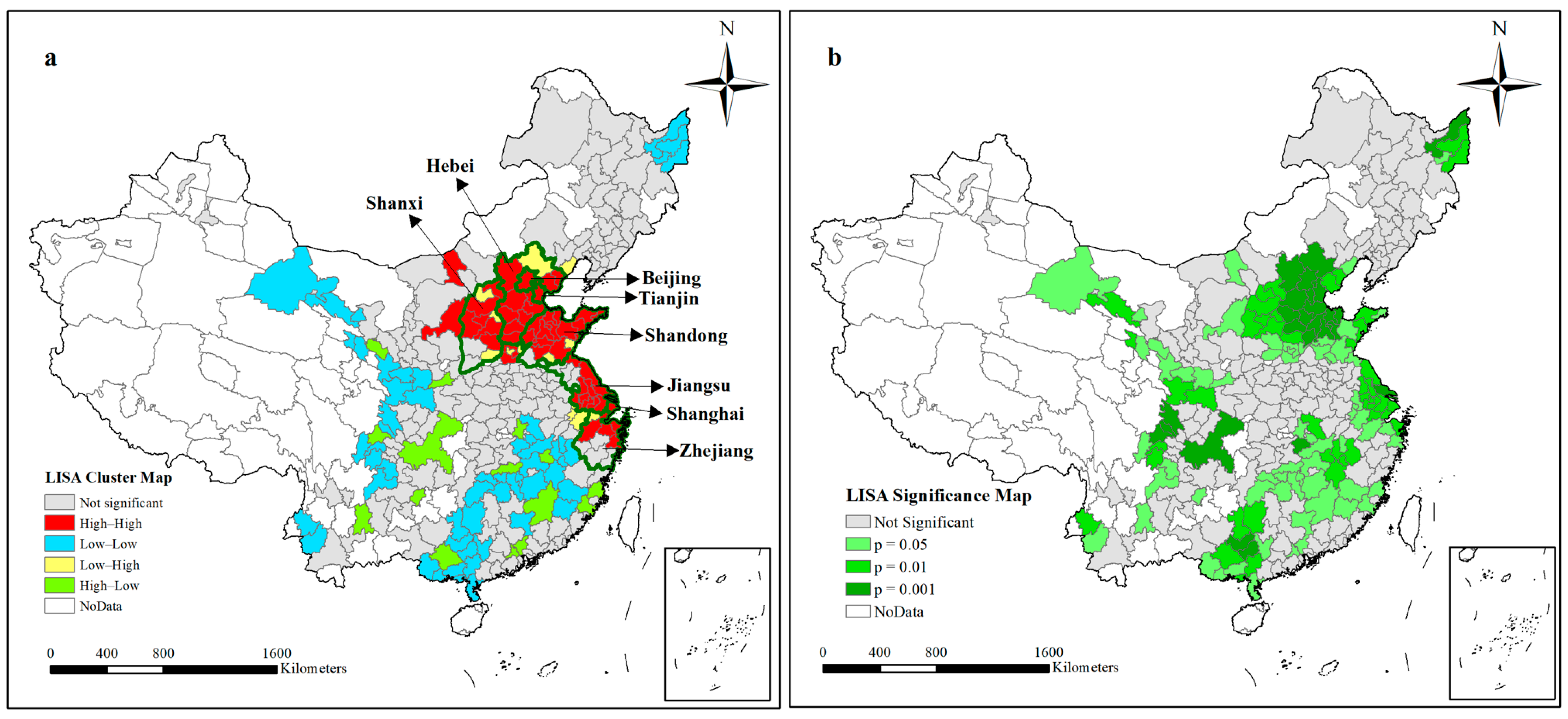
Figure 3, many cities are shown in red or blue in the local indicators of spatial autocorrelation (LISA) cluster map, indicating the high–high or low–low spatial clustering. A total of 132 cities show significant spatial dependence in the LISA significance map, while others are not significantly spatially dependent.
First, the Beijing–Tianjin–Hebei region and the Yangtze River Delta region exhibit a significant high–high clustering. With Beijing and Shanghai as the two centers, the significance gradually decreases outwards. This suggests that the cities with high carbon emissions in China are mainly clustered in these two regions, and they have a stronger spatial dependence the closer they are to the two core cities. However, spatial dependence may change when the study area is narrowed from the national to regional scale. The carbon emissions of cities in the Yellow River Economic Belt showed significant clustering characteristics in the spatial autocorrelation analysis, but high–high clusters were mainly concentrated in Shandong Peninsula, while low–low clusters were distributed in the upstream and midstream of the Yellow River [46]. In Yangtze River Delta cities, the maximum Global Moran’s I was only 0.071, implying a weak trend of spatial aggregation of urban carbon emissions [6]. The scope on a national scale is more conducive to highlighting regional characteristics and comparing differences between regions. In addition, the cities with low–low clusters are mainly concentrated in Southwest and Heilongjiang province. Panzhihua in Sichuan Province, Liuzhou in Guangxi Zhuang Autonomous Region, and Shuangyu and Jiamusi in Heilongjiang Province are highly significant, but do not form a clear center due to their fragmented distribution. This means that the cities with low carbon emissions are mainly clustered in the Southwest and Northeast and are evenly distributed, which is consistent with previous studies. Finally, cities with high–low and low–high clustering are mainly distributed at the edges of high- (low-) carbon-emissions-clustering city blocks, without forming significant spatial aggregation.

4.4. Results of SEM and OLS

As shown in Table 4, for the 282 cities in the study area, SEM has a higher log likelihood and lower Akaike information criterion than OLS, which indicates that SEM fits the data better. Meanwhile, the R2 of SEM and OLS is 76% and 73%, respectively, so SEM can explain carbon emissions better.
The coefficients of CA, PARA-MN and ENN-MN are 0.800, 0.322 and 0.202, respectively, showing a significant positive correlation with carbon emissions. This means that the growth in urban areas, irregularity of morphology and urban sprawl all increase carbon emissions, and the effect of urban areas on carbon emissions is much greater than irregularity and sprawl. In contrast, the coefficient of PROX-MN is −0.293, which shows a significant negative correlation with carbon emissions. This suggests that an increase in urban segregation and fragmentation will increase carbon emissions. At the same time, the results support the hypothesis that urban form landscape metrics affect carbon emissions.
In the spatial autocorrelation test for each region, there is no significant spatial dependence in the North, Southwest and Mid-South regions. There is significant spatial dependence in the East, Northwest and Northeast regions, but the Lagrange Multiplier (lag) and Lagrange Multiplier (error) of these regions are insignificant, indicating that OLS should be used to analyze the effects of urban form on carbon emissions in these regions. Therefore, OLS is more suitable for use in regional analysis than SEM.
The results of OLS for different regions are shown in Table 5. The variables that are significant in each region (p ≤ 0.05), are selected for the next analysis. CA has a significant positive correlation with carbon emissions in all regions, with the highest coefficient of 1.253 in Southwest. As the sizes of cities increase, the influence of the area on carbon emissions decreases [13]. PARA-MN shows a significant positive correlation with a coefficient of 0.231 and 0.358 in the Northeast and East, respectively. PROX-MN shows a significant negative correlation with a coefficient of −0.752 and −0.241 in the North and Mid-South, respectively. Sha et al. [28] not only found this result by studying 232 cities in China during 2000–2010, but also concluded that this phenomenon is more obvious in coastal areas. However, it is worth noting that the value of PROX-MN in the East is 0.114, indicating an upward trend in carbon emissions as urban compactness grows in the East region. Considering this metric has no significant effect on carbon emissions, the phenomenon will not be discussed next. However, the results can provide a direction for future research, especially the impact of compact cities on carbon emissions. ENN-MN shows a significant positive correlation with a coefficient of 0.566 for urban carbon emissions in the North. The above results support the hypothesis that the effect of each metric varies from region to region.

4.5. Discussion

4.5.1. Mechanisms of the Effects of Urban Form on Carbon Emissions

CA shows a positive correlation with carbon emissions in all 282 cities, implying that the expansion of urban areas can increase carbon emissions. Urban growth does not directly lead to the increase in carbon emissions, but it can increase economic opportunities, population growth and commuting distances, which have been closely linked to carbon emissions. Urban areas, economy and ecology are the core issues for achieving sustainable development in complex geographic areas, and the growth of urban areas has positive effects on economic development and carbon emissions [47]. However, as the city grows, the ecology in general moves in a positive direction. Wang et al. [48] found that urbanization plays a positive mediating effect in the impact of financial scale and financial efficiency on carbon emissions, and this mediating effect includes both chain and parallel effects. Then, although there is a U-type relationship between urbanization and carbon emissions intensity [14], China is currently in the process of rapid urbanization. The rate of urbanization in some developed cities is gradually slowing down, but more cities are still in the first half of the U-shape. Thus, we were able to establish that urban area affects urban carbon emissions through various factors.
PARA-MN shows a significant positive effect on carbon emissions in the Northeast and East, implying that irregular urban development can increase carbon emissions. Regional policies are the key factors contributing to this effect. After the 16th Communist Party Congress, the Northeast region began to revive the old industrial bases and enhance development efforts in specific regions, such as the Liaoning coastal economic belt, Shenyang economic zone and Hadazhi industrial corridor. During the implementation of the policy, the government strengthened infrastructure development and restructured the state-owned enterprises, but there were still a lot of land sales. On the one hand, this has exacerbated the low-density extension of some cities I then Northeast, leading to irregular urban expansion [49]. On the other hand, there are a large number of resource-dependent cities. These resource-dependent cities are mainly located around capital cities and dominated by secondary industries. While the spatial distribution range expands, the population and economy shrink, generating more carbon emissions than other types of cities. Finally, the irregular shape of the city also affects the traffic road network in the East region. The irregular development of cities increases the development of inter-regional long-range transport situations and intensifies the emission of CO2.
PROX-MN shows a significant negative effect on carbon emissions in the North and Mid-South, implying that compact urban development can reduce carbon emissions. The North and Mid-South regions of China are in the stage of rapid urban development. Influenced by urban planning, the cities in these regions are beginning to develop into compact cities. The compact city can improve land use efficiency and reduce commuting distances. It has been proven to be a more useful form to reduce carbon emissions compared to the scattered patterns of early urban development [50]. Thus, the focus of our compact city policy is to maximize the strengths and minimize the weaknesses to capture the best shape of compact cities. However, compact cities may not always be the best form for reducing carbon emissions according to the experience of foreign urban development. For example, the concentration of population beyond a certain level will consume a lot of resources and increase per capita carbon emissions [28].
ENN-MN shows a significant positive effect on carbon emissions in the North. Urban expansion has a deeper connotation than the growth in area, which means that cities gradually shift from outward expansion to inward development. Si et al. [51] also found that in the North, urbanization has the most significant impact on carbon emissions than other regions, followed by the consumption of fossil energy. The cities in the North have higher intra-urban land use, a large concentration of people and industries in a smaller land area, and high transportation density, which results in more significant carbon emissions from urban expansion than other regions. For example, Tianjin has been transformed from a production city to a consumption city since 2000, and investments in industrial infrastructure have generated the most carbon emissions [52]. An integrated model consisting of population, income and urbanization can better explain the growth in carbon emissions.

4.5.2. Policy Implications for Low-Carbon Urban Planning

According to the effects of urban size, complexity, compactness and centrality on carbon emissions, the region-specific policy recommendations regarding low-carbon urban planning are as follows.
First, based on the significant positive effect of urban area on carbon emissions and the significant negative effect of urban compactness on carbon emissions in the North and Mid-South, the selection of appropriate urban development patterns is a key aspect of low-carbon urban planning in China. Currently, there is still a gap in the urbanization level between China and the developed countries, especially in some cities in the Northwest, Southwest and Mid-South. Therefore, the focus of urban development at this stage remains on compact development, improving the efficiency of land and public facilities utilization, and avoiding blind expansion. However, when urban compactness exceeds a certain threshold, we also need to consider the issues of traffic, population density and health. On the one hand, we need to develop specific measures for different cities to maintain urban compactness at an appropriate level, so as to achieve the goal of maintaining low carbon emissions while living in a livable environment, for example, by balancing the relationship between urban compactness, water bodies and green spaces to achieve the coexistence of regulated urban microclimates and compact cities [53]. On the other hand, future urban development can also shift towards other urban forms, such as polycentric development. It can improve carbon efficiency while reducing traffic pressure and is suitable for cities with large populations in China [28].
Second, based on the significant positive effect of urban expansion on carbon emissions and the spatial characteristics in the North, low-carbon urban planning should focus on optimizing the energy structure and improving energy use efficiency. Above all, population and technology are prerequisites for improving energy efficiency. The North region should use its regional attractiveness and combine it with the national strategy of “One Belt, One Road” to increase the inflow of highly qualified personnel and the import of high technology. The development of a low-carbon transportation system is also an important aspect. Transportation carbon emissions caused by decentralized urban distribution should be reduced through rational transportation and road network planning. Transportation planning should shift from quantity to quality and from building more roads to optimizing the structure of the road system. Public transportation, as one of the main sources of carbon emissions from transportation, produces less carbon emissions than private cars. Thus, it is necessary to increase the number of public car and subway operating stations and reasonably limit the amount of private car ownership [54]. Finally, the North region is at the key node of domestic industrial transfers and needs to ensure that pollution does not occur again. To reduce the vicious competition in the process of industrial transfers, relevant planning is needed to restrict companies. Companies also need to optimize their development for energy-intensive industries, shifting from a focus on coal resources to cleaner energy sources and technological innovation. Cities need to seize the important opportunity period of industry shifts to eliminate outdated production equipment and develop a reasonable strategy for future industrial development.
Third, based on the significant positive effect of urban complexity on carbon emissions in the Northeast and East, the government should pay attention to urban development boundary control in its planning. In the context of China’s current territorial spatial planning, the government needs to strengthen the control of urban development boundaries. The control of these boundaries mainly includes the formulation of growth boundaries and the delineation of urban areas. The growth boundary should be set with attention to both the rigid boundary of a reasonable scale and the flexible boundary of the reuse of the internal stock of land. Then, the cities should choose the appropriate development boundary orientation, combining their stage of development and existing problems. For example, Sargent et al. [55] detected changes in carbon emissions around Boston by combining CO2 emissions inventories and Lagrangian particle dispersion models, which were used to assess carbon mitigation efforts in the surrounding area and establish buffer zones.

5. Conclusions

This study identified the set of urban form landscape metrics, then analyzed the characteristics and spatial correlation of carbon emissions in 282 cities in China and used a spatial error model to analyze the effects of urban form on carbon emissions. First, through stepwise linear regression, the set of urban form landscape metrics was determined to include the four metrics of CA, PARA-MN, PROX-MN and ENN-MN. In addition, there is a significant positive spatial autocorrelation within the study area. Through Local Moran’s I, it was found that cities with high (low) carbon emissions are more likely to cluster spatially. The cities with high–high clustering are mainly clustered in the Beijing–Tianjin–Hebei region and the Yangtze River Delta region. The low–low clustering cities are mainly concentrated in the Southwest and Heilongjiang Province. Furthermore, the results of the spatial error model reveal that CA, PARA-MN and ENN-MN show a significant positive correlation with carbon emissions, and the most significant effect for urban areas among the three. In contrast, PROX-MN shows a significant negative correlation with carbon emissions. By dividing cities into administrative divisions, CA shows a significant positive correlation in all regions, and the highest coefficient in the Northwest, which is related to the economic growth and population increase that occurs as urban areas grow. PARA-MN has a significant positive correlation in the Northeast and East, which is related to regional planning and traffic. PROX-MN has a significant negative correlation in the North and Mid-South, which is related to the rapid urbanization development of these cities. ENN-MN has a significant positive correlation only in the North, which is related to the high land utilization rate and dense population resources of cities in the North. These results strongly support the validity of the hypotheses. Finally, based on the effects of urban form on carbon emissions, we proposed recommendations for low-carbon urban planning, including selecting appropriate urban development patterns, strengthening energy structure optimization and utilization efficiency, and strengthening urban development boundary control.
This study has some research limitations. Firstly, limited by the availability of data, the data used only contain urban impervious surfaces and therefore do not allow for the identification of detailed land use types. By exploring the effects of the urban form on carbon emissions as influenced by different land use types, it can help to suggest low-carbon planning recommendations specific to the land use type. Future work will identify the different land use types. Secondly, this study classifies cities according to their geographical location and ultimately finds that PROX-MN in the East has the opposite effect on carbon emissions compared to other regions. For this particular result, we need to extend the time scale in future work and focus on the coefficient of PROX-MN in the East.

Author Contributions

Conceptualization, S.Z.; Data curation, Y.H. and Y.S.; Formal analysis, Y.H. and Y.S.; Funding acquisition, S.Z.; Methodology, S.Z., Y.H. and Y.S.; Supervision, S.Z.; Validation, Y.H. and Y.S.; Writing—original draft, S.Z., Y.H. and Y.S.; Writing—review & editing, S.Z. and Y.H. All authors have read and agreed to the published version of the manuscript.

Funding

This research was funded by the National Natural Science Foundation of China (Grant No. 42007194), and the Open Fund of Key Laboratory of Urban Land Resources Monitoring and Simulation, Ministry of Natural Resources (Grant No. KF-2021-06-068).

Institutional Review Board Statement

Not applicable.

Informed Consent Statement

Not applicable.

Data Availability Statement

The data in the article are detailed in Section 2.2. All the data used are reflected in the article. If you need other relevant data, please contact the authors.

Acknowledgments

The authors are grateful to Chen et al. (https://www.ceads.net.cn/data/county/ (accessed on 1 April 2022)) for the carbon emissions data in China. The authors are grateful to Gong et al. (http://data.ess.tsinghua.edu.cn (accessed on 1 April 2022)) for the urban impervious surface data in China.

Conflicts of Interest

The authors declare no conflict of interest.

Appendix A

We selected 15 landscape metrics and described them briefly. The equations and specific descriptions of these metrics are given in Table A1 in order to improve comprehension of the metric selection.
Table A1. Urban form landscape metric system.
CategoryVariableEquationDescription
AreaClass Area (CA) CA = i = 1 n a i ( 1 10000 ) Urban area
Number of Patches (NP) NP = n Urban fragmentation
Largest Patch Index (LPI) LPI = max j = 1 n ( a ij ) CA 100 Urban growth
EdgeEdge density (ED) ED = i = 1 n e i CA Urban shape complexity
ShapeArea-weighted Mean Shape Index (AWMSI) AWMSI = i = 1 m j = 1 n [ ( p ij minp ij ) ( a ij CA ) ] Urban shape complexity
Area-weighted Mean Patch Fractal Dimension (AWMPFD) AWMPFD = i = 1 m j = 1 n [ ( 2 ln ( 0 . 25 p ij ) ln ( a ij ) ) ( a ij CA ) ] Urban shape complexity
Mean Perimeter–Area Ratio (PARA-MN) PARA-MN = i = 1 m j = 1 n ( p ij a ij ) mn Urban shape complexity
AggregationLandscape Shape Index (LSI) LSI = 0.25 k = 1 m e ik * CA Urban shape complexity
Clumpiness Index (CLUMPY) CLUMPY = [ G i P i P i ] if   G i < P i < 0.5   else
CLUMPY = [ G i P i 1 P i ]
Urban compactness
Percentage of Like Adjacencies (PLADJ) PLADJ = ( i = 1 m g ii i = 1 m k = 1 n g ik ) ( 100 ) Urban compactness
Patch Cohesion Index (COHESION) COHESION = [ 1 i = 1 m j = 1 n p ij * i = 1 m j = 1 n p ij * a ij * ] × [ 1 1 Z ] 1 (100)Urban compactness
Aggregation Index (AI) AI = [ g ii max ( g ii ) ] ( 100 ) Urban compactness
Mean Proximity Index (PROX-MN) PROX-MN = s = 1 n a ijs h ijs Urban compactness
Mean Euclidian Nearest Neighbor Distance (ENN-MN) ENN-MN = h ij Centrality
Patch Density (PD) PD = n CA Urban fragmentation

Appendix B

Before determining the spatial econometric model, it is necessary to diagnose the spatial dependence of urban form and carbon emissions. Comparing the spatial regression statistics in Table A2, both Lagrange Multiplier (lag) and Lagrange Multiplier (error) are significant (p < 0.05), but P (Robust LM (lag)) = 0.120 > 0.1, p (Robust LM (error)) = 0.000 < 0.01, and value (Robust LM (lag)) < value (Robust LM (error)), so the spatial error model is the better choice.
Table A2. Diagnostics for spatial dependence of urban form and carbon emissions.
TestDegree of FreedomValueProbability
Lagrange Multiplier (lag)14.3390.037
Robust LM (lag)12.4170.120
Lagrange Multiplier (error)138.2790.000
Robust LM (error)136.3580.000

References

  1. Li, B.; Gasser, T.; Ciais, P.; Piao, S.; Tao, S.; Balkanski, Y.; Hauglustaine, D.; Boisier, J.-P.; Chen, Z.; Huang, M.; et al. The Contribution of China’s Emissions to Global Climate Forcing. Nature 2016, 531, 357–361. [Google Scholar] [CrossRef]
  2. Mi, Z.; Meng, J.; Guan, D.; Shan, Y.; Song, M.; Wei, Y.-M.; Liu, Z.; Hubacek, K. Chinese CO2 Emission Flows Have Reversed since the Global Financial Crisis. Nat. Commun. 2017, 8, 1712. [Google Scholar] [CrossRef] [PubMed]
  3. Dale, S. BP Statistical Review of World Energy 2021, 70th ed.; BP Plc: London, UK, 2021; Available online: https://www.bp.com/en/global/corporate/energy-economics/statistical-review-of-world-energy/co2-emissions.html (accessed on 1 April 2022).
  4. Tong, X.; Guo, S.; Duan, H.; Duan, Z.; Gao, C.; Chen, W. Carbon-Emission Characteristics and Influencing Factors in Growing and Shrinking Cities: Evidence from 280 Chinese Cities. Int. J. Environ. Res. Public. Health 2022, 19, 2120. [Google Scholar] [CrossRef] [PubMed]
  5. Liu, C.; Liang, Y.; Zhao, Y.; Liu, S.; Huang, C. Simulation and Analysis of the Effects of Land Use and Climate Change on Carbon Dynamics in the Wuhan City Circle Area. Int. J. Environ. Res. Public Health 2021, 18, 11617. [Google Scholar] [CrossRef] [PubMed]
  6. Liu, H.; Nie, J.; Cai, B.; Cao, L.; Wu, P.; Pang, L.; Wang, X. CO2 Emissions Patterns of 26 Cities in the Yangtze River Delta in 2015: Evidence and Implications. Environ. Pollut. 2019, 252, 1678–1686. [Google Scholar] [CrossRef]
  7. Cai, B.; Zhang, L. Urban CO2 Emissions in China: Spatial Boundary and Performance Comparison. Energy Policy 2014, 66, 557–567. [Google Scholar] [CrossRef]
  8. Huang, C.; Qu, Y.; Huang, L.; Meng, X.; Chen, Y.; Pan, P. Quantifying the Impact of Urban Form and Socio-Economic Development on China’s Carbon Emissions. Int. J. Environ. Res. Public. Health 2022, 19, 2976. [Google Scholar] [CrossRef]
  9. Liu, S.; Liao, Q.; Liang, Y.; Li, Z.; Huang, C. Spatio–Temporal Heterogeneity of Urban Expansion and Population Growth in China. Int. J. Environ. Res. Public Health 2021, 18, 13031. [Google Scholar] [CrossRef]
  10. Christen, A.; Coops, N.C.; Crawford, B.R.; Kellett, R.; Liss, K.N.; Olchovski, I.; Tooke, T.R.; van der Laan, M.; Voogt, J.A. Validation of Modeled Carbon-Dioxide Emissions from an Urban Neighborhood with Direct Eddy-Covariance Measurements. Atmos. Environ. 2011, 45, 6057–6069. [Google Scholar] [CrossRef]
  11. Ewing, R.; Rong, F. The Impact of Urban Form on U.S. Residential Energy Use. Hous. Policy Debate 2008, 19, 1–30. [Google Scholar] [CrossRef]
  12. Palme, M.; Inostroza, L.; Villacreses, G.; Lobato-Cordero, A.; Carrasco, C. From Urban Climate to Energy Consumption. Enhancing Building Performance Simulation by Including the Urban Heat Island Effect. Energy Build. 2017, 145, 107–120. [Google Scholar] [CrossRef]
  13. Shi, K.; Xu, T.; Li, Y.; Chen, Z.; Gong, W.; Wu, J.; Yu, B. Effects of Urban Forms on CO2 Emissions in China from a Multi-Perspective Analysis. J. Environ. Manag. 2020, 262, 110300. [Google Scholar] [CrossRef] [PubMed]
  14. Ding, Y.; Li, F. Examining the Effects of Urbanization and Industrialization on Carbon Dioxide Emission: Evidence from China’s Provincial Regions. Energy 2017, 125, 533–542. [Google Scholar] [CrossRef]
  15. Zhang, C.; Chen, P. Industrialization, Urbanization, and Carbon Emission Efficiency of Yangtze River Economic Belt—Empirical Analysis Based on Stochastic Frontier Model. Environ. Sci. Pollut. Res. 2021, 28, 66914–66929. [Google Scholar] [CrossRef]
  16. Wang, G.; Han, Q.; de Vries, B. Assessment of the Relation between Land Use and Carbon Emission in Eindhoven, the Netherlands. J. Environ. Manag. 2019, 247, 413–424. [Google Scholar] [CrossRef]
  17. Qin, H.; Huang, Q.; Zhang, Z.; Lu, Y.; Li, M.; Xu, L.; Chen, Z. Carbon Dioxide Emission Driving Factors Analysis and Policy Implications of Chinese Cities: Combining Geographically Weighted Regression with Two-Step Cluster. Sci. Total Environ. 2019, 684, 413–424. [Google Scholar] [CrossRef]
  18. Chen, B.; Xu, C.; Wu, Y.; Li, Z.; Song, M.; Shen, Z. Spatiotemporal Carbon Emissions across the Spectrum of Chinese Cities: Insights from Socioeconomic Characteristics and Ecological Capacity. J. Environ. Manag. 2022, 306, 114510. [Google Scholar] [CrossRef]
  19. Li, C.; Li, H.; Qin, X. Spatial Heterogeneity of Carbon Emissions and Its Influencing Factors in China: Evidence from 286 Prefecture-Level Cities. Int. J. Environ. Res. Public Health 2022, 19, 1226. [Google Scholar] [CrossRef]
  20. Urquizo, J.; Calderón, C.; James, P. Metrics of Urban Morphology and Their Impact on Energy Consumption: A Case Study in the United Kingdom. Energy Res. Soc. Sci. 2017, 32, 193–206. [Google Scholar] [CrossRef]
  21. Chen, Y.-J.; Matsuoka, R.H.; Liang, T.-M. Urban Form, Building Characteristics, and Residential Electricity Consumption: A Case Study in Tainan City. Environ. Plan. B Urban Anal. City Sci. 2018, 45, 933–952. [Google Scholar] [CrossRef]
  22. Khalifa, M.; Elagib, N.A.; Ribbe, L.; Schneider, K. Spatio-Temporal Variations in Climate, Primary Productivity and Efficiency of Water and Carbon Use of the Land Cover Types in Sudan and Ethiopia. Sci. Total Environ. 2018, 624, 790–806. [Google Scholar] [CrossRef]
  23. Wang, F.; Wang, G.; Liu, J.; Chen, H. How Does Urbanization Affect Carbon Emission Intensity under a Hierarchical Nesting Structure? Empirical Research on the China Yangtze River Delta Urban Agglomeration. Environ. Sci. Pollut. Res. 2019, 26, 31770–31785. [Google Scholar] [CrossRef] [PubMed]
  24. Falahatkar, S.; Rezaei, F. Towards Low Carbon Cities: Spatio-Temporal Dynamics of Urban Form and Carbon Dioxide Emissions. Remote Sens. Appl. Soc. Environ. 2020, 18, 100317. [Google Scholar] [CrossRef]
  25. Fang, C.; Wang, S.; Li, G. Changing Urban Forms and Carbon Dioxide Emissions in China: A Case Study of 30 Provincial Capital Cities. Appl. Energy 2015, 158, 519–531. [Google Scholar] [CrossRef]
  26. Li, T.; Xu, Y.; Yao, L. Detecting Urban Landscape Factors Controlling Seasonal Land Surface Temperature: From the Perspective of Urban Function Zones. Environ. Sci. Pollut. Res. 2021, 28, 41191–41206. [Google Scholar] [CrossRef]
  27. Zhang, P.; Yang, L.; Ma, W.; Wang, N.; Wen, F.; Liu, Q. Spatiotemporal Estimation of the PM2.5 Concentration and Human Health Risks Combining the Three-Dimensional Landscape Pattern Index and Machine Learning Methods to Optimize Land Use Regression Modeling in Shaanxi, China. Environ. Res. 2022, 208, 112759. [Google Scholar] [CrossRef]
  28. Sha, W.; Chen, Y.; Wu, J.; Wang, Z. Will Polycentric Cities Cause More CO2 Emissions? A Case Study of 232 Chinese Cities. J. Environ. Sci. 2020, 96, 33–43. [Google Scholar] [CrossRef]
  29. Wang, Z.; Chen, J.; Zhou, C.; Wang, S.; Li, M. The Impacts of Urban Form on PM2.5 Concentrations: A Regional Analysis of Cities in China from 2000 to 2015. Atmosphere 2022, 13, 963. [Google Scholar] [CrossRef]
  30. Yang, B.; Bai, Z.; Wang, J. Spatiotemporal Dynamic Differences of Energy-Related CO2 Emissions and the Related Driven Factors in Six Regions of China during Two Decades. Environ. Sci. Pollut. Res. 2022, 29, 24737–24756. [Google Scholar] [CrossRef]
  31. Chen, J.; Gao, M.; Cheng, S.; Hou, W.; Song, M.; Liu, X.; Liu, Y.; Shan, Y. County-Level CO2 Emissions and Sequestration in China during 1997–2017. Sci. Data 2020, 7, 391. [Google Scholar] [CrossRef]
  32. Jia, Y.; Tang, L.; Xu, M.; Yang, X. Landscape Pattern Indices for Evaluating Urban Spatial Morphology–A Case Study of Chinese Cities. Ecol. Indic. 2019, 99, 27–37. [Google Scholar] [CrossRef]
  33. Gong, P.; Li, X.; Zhang, W. 40-Year (1978–2017) Human Settlement Changes in China Reflected by Impervious Surfaces from Satellite Remote Sensing. Sci. Bull. 2019, 64, 756–763. [Google Scholar] [CrossRef]
  34. Fei, W.; Zhao, S. Urban Land Expansion in China’s Six Megacities from 1978 to 2015. Sci. Total Environ. 2019, 664, 60–71. [Google Scholar] [CrossRef] [PubMed]
  35. Li, C.; Li, J.; Wu, J. Quantifying the Speed, Growth Modes, and Landscape Pattern Changes of Urbanization: A Hierarchical Patch Dynamics Approach. Landsc. Ecol. 2013, 28, 1875–1888. [Google Scholar] [CrossRef]
  36. Deng, H.; Zhang, K.; Wang, F.; Dang, A. Compact or Disperse? Evolution Patterns and Coupling of Urban Land Expansion and Population Distribution Evolution of Major Cities in China, 1998–2018. Habitat Int. 2021, 108, 102324. [Google Scholar] [CrossRef]
  37. Clark, L.P.; Millet, D.B.; Marshall, J.D. Air Quality and Urban Form in U.S. Urban Areas: Evidence from Regulatory Monitors. Environ. Sci. Technol. 2011, 45, 7028–7035. [Google Scholar] [CrossRef]
  38. Wang, Y.; Zheng, Y. Spatial Effects of Carbon Emission Intensity and Regional Development in China. Environ. Sci. Pollut. Res. 2021, 28, 14131–14143. [Google Scholar] [CrossRef]
  39. Liu, X.; Ming, Y.; Liu, Y.; Yue, W.; Han, G. Influences of Landform and Urban Form Factors on Urban Heat Island: Comparative Case Study between Chengdu and Chongqing. Sci. Total Environ. 2022, 820, 153395. [Google Scholar] [CrossRef]
  40. Wang, Z.; Li, Y.; Cai, H.; Wang, B. Comparative Analysis of Regional Carbon Emissions Accounting Methods in China: Production-Based versus Consumption-Based Principles. J. Clean. Prod. 2018, 194, 12–22. [Google Scholar] [CrossRef]
  41. Liu, X.; Zhang, L.; Hao, Y.; Yin, X.; Shi, Z. Increasing Disparities in the Embedded Carbon Emissions of Provincial Urban Households in China. J. Environ. Manag. 2022, 302, 113974. [Google Scholar] [CrossRef]
  42. Xu, L.; Chen, G.; Wiedmann, T.; Wang, Y.; Geschke, A.; Shi, L. Supply-Side Carbon Accounting and Mitigation Analysis for Beijing-Tianjin-Hebei Urban Agglomeration in China. J. Environ. Manag. 2019, 248, 109243. [Google Scholar] [CrossRef] [PubMed]
  43. Zhao, W.; Liu, X.; Deng, Q.; Li, D.; Xu, J.; Li, M.; Cui, Y. Spatial Association of Urbanization in the Yangtze River Delta, China. Int. J. Environ. Res. Public Health 2020, 17, 7276. [Google Scholar] [CrossRef] [PubMed]
  44. Tang, D.; Zhang, Y.; Bethel, B.J. A Comprehensive Evaluation of Carbon Emission Reduction Capability in the Yangtze River Economic Belt. Int. J. Environ. Res. Public Health 2020, 17, 545. [Google Scholar] [CrossRef] [PubMed]
  45. Zhang, X.; Zhao, Y. Identification of the Driving Factors’ Influences on Regional Energy-Related Carbon Emissions in China Based on Geographical Detector Method. Environ. Sci. Pollut. Res. 2018, 25, 9626–9635. [Google Scholar] [CrossRef] [PubMed]
  46. Zhang, J.; Feng, Y.; Zhu, Z. Spatio-Temporal Heterogeneity of Carbon Emissions and Its Key Influencing Factors in the Yellow River Economic Belt of China from 2006 to 2019. Int. J. Environ. Res. Public Health 2022, 19, 4185. [Google Scholar] [CrossRef]
  47. Han, Z.; Jiao, S.; Zhang, X.; Xie, F.; Ran, J.; Jin, R.; Xu, S. Seeking Sustainable Development Policies at the Municipal Level Based on the Triad of City, Economy and Environment: Evidence from Hunan Province, China. J. Environ. Manag. 2021, 290, 112554. [Google Scholar] [CrossRef]
  48. Wang, F.; Fan, W.; Chen, C.; Liu, J.; Chai, W. The Dynamic Time-Varying Effects of Financial Development, Urbanization on Carbon Emissions in the Yangtze River Delta, China. Environ. Sci. Pollut. Res. 2019, 26, 14226–14237. [Google Scholar] [CrossRef]
  49. Wang, Y. Development Characteristics, Influencing Mechanism and Coping Strategies of Resource-Based Cities in Developing Countries: A Case Study of Urban Agglomeration in Northeast China. Environ. Sci. Pollut. Res. 2022, 29, 25336–25348. [Google Scholar] [CrossRef]
  50. Wu, H.; Fang, S.; Zhang, C.; Hu, S.; Nan, D.; Yang, Y. Exploring the Impact of Urban Form on Urban Land Use Efficiency under Low-Carbon Emission Constraints: A Case Study in China’s Yellow River Basin. J. Environ. Manag. 2022, 311, 114866. [Google Scholar] [CrossRef]
  51. Siqin, Z.; Niu, D.; Li, M.; Zhen, H.; Yang, X. Carbon Dioxide Emissions, Urbanization Level, and Industrial Structure: Empirical Evidence from North China. Environ. Sci. Pollut. Res. 2022, 29, 34528–34545. [Google Scholar] [CrossRef]
  52. Zhang, Y.; Bai, H.; Hou, H.; Zhang, Y.; Xu, H.; Ji, Y.; He, G.; Zhang, Y. Exploring the Consumption-Based Carbon Emissions of Industrial Cities in China: A Case Study of Tianjin. Environ. Sci. Pollut. Res. 2021, 28, 26948–26960. [Google Scholar] [CrossRef] [PubMed]
  53. Koch, F.; Bilke, L.; Helbig, C.; Schlink, U. Compact or Cool? The Impact of Brownfield Redevelopment on Inner-City Micro Climate. Sustain. Cities Soc. 2018, 38, 31–41. [Google Scholar] [CrossRef]
  54. Dong, F.; Wang, Y.; Zhang, X. Can Environmental Quality Improvement and Emission Reduction Targets Be Realized Simultaneously? Evidence from China and A Geographically and Temporally Weighted Regression Model. Int. J. Environ. Res. Public Health 2018, 15, 2343. [Google Scholar] [CrossRef]
  55. Sargent, M.; Barrera, Y.; Nehrkorn, T.; Hutyra, L.R.; Gately, C.K.; Jones, T.; McKain, K.; Sweeney, C.; Hegarty, J.; Hardiman, B.; et al. Anthropogenic and Biogenic CO2 Fluxes in the Boston Urban Region. Proc. Natl. Acad. Sci. USA 2018, 115, 7491–7496. [Google Scholar] [CrossRef] [PubMed]
Figure 1. Distribution of 282 cities in six regions in China.
Land 11 01343 g001
Figure 2. Distribution of carbon emissions in 282 cities.
Land 11 01343 g002
Figure 3. The local spatial autocorrelation of carbon emissions in 282 cities in 2017: (a) the local indicators of spatial autocorrelation (LISA) cluster map; (b) LISA significance map. Note: In the LISA significance map, p = 0.001 indicates significance at the 1‰ level, p = 0.01 indicates significance at the 1% level, p = 0.05 indicates significance at the 5% level. If the significance level is below 5%, the city passes the significance test.
Land 11 01343 g003
Table 1. Multicollinearity test results statistics.
Landscape MetricsCollinearity StatisticsLandscape MetricsCollinearity Statistics
ToleranceVIFToleranceVIF
CA0.04124.658CLUMPY0.003372.238
NP0.02343.959PLADJ0.0008627.861
LPI0.05318.816COHESION0.07213.827
ED0.007134.318AI0.0009250.508
AWMSI0.03727.091PROX-MN0.1029.769
AWMPFD0.03429.444ENN-MN0.2633.802
PARA-MN0.2094.782PD0.02934.254
LSI0.01567.847---
Note: VIF: the variance inflation factors; CA: Class Area; NP: the Number of Patches; LPI: the Largest Patch Index; ED: Edge Density; AWMSI: the Area-weighted Mean Shape Index; AWMPFD: the Area-weighted Mean Patch Fractal Dimension; PARA-MN: Mean Perimeter–Area Ratio; LSI: the Landscape Shape Index; CLUMPY: the Clumpiness Index; PLADJ: the Percentage of Like Adjacencies; COHESION: the Patch Cohesion Index; AI: the Aggregation Index; PROX-MN: the Proximity Index; ENN-MN: the Euclidian Mean Nearest Neighbor Distance; PD: Patch Density.
Table 2. Stepwise linear regression model results statistics.
VariableCoefficientVIF
Constant−0.314 ***-
CA0.796 ***1.534
PROX-MN−0.331 ***1.437
PARA-MN0.350 ***3.055
ENN-MN0.182 ***2.534
CLUMPY0.093 ***1.871
R20.739
Adjusted R20.734
FF = 155.968, p = 0.000
Note: *** indicates significance at 1% level. F: F-test statistic value.
Table 3. Result statistics of urban form metrics.
AreaStatisticsCarbon EmissionsCAPARA-MNPROX-MNENN-MN
All AreasMin0.00000.00000.00000.00000.0000
Max1.00001.00001.00001.00001.0000
Mean0.14020.16110.82220.03460.0500
Std0.13420.16540.11470.08580.1119
NorthMin0.06830.05930.55280.00160.0068
Max0.77411.00000.86380.28100.6036
Mean0.26680.26120.78080.04600.0467
Std0.15710.21320.07010.06830.1045
NortheastMin0.00920.02250.00000.00230.0150
Max0.41050.35480.93730.29601.0000
Mean0.11030.10860.71610.03280.1801
Std0.08820.08460.24840.05800.2569
EastMin0.01500.02260.69030.00060.0023
Max1.00000.95530.92420.23510.0469
Mean0.16970.23800.81870.03150.0177
Std0.14790.18770.04570.04730.0107
Mid-SouthMin0.00160.01380.70480.00090.0000
Max0.44950.65620.94491.00000.0787
Mean0.10690.13630.84890.04850.0253
Std0.08330.12920.05910.13870.0139
SouthwestMin0.00000.00000.86260.00000.0148
Max0.79380.59860.94980.06360.1121
Mean0.09870.07580.90900.00850.0409
Std0.15490.11990.02180.01530.0211
NorthwestMin0.00600.01090.53960.00050.0013
Max0.32370.35761.00000.32940.3938
Mean0.09540.07660.83200.02530.0609
Std0.08570.08340.09370.06030.0799
Note: Min: minimum value; Max: maximum value; Std: standard deviation.
Table 4. Comparison between ordinary least squares (OLS) and spatial error model (SEM) results.
VariableOLSSEM
Constant−0.208 ***−0.253 ***
CA0.777 ***0.800 ***
PARA-MN0.271 ***0.322 ***
PROX-MN−0.289 ***−0.293 ***
ENN-MN0.199 ***0.202 ***
LAMBDA-0.557 ***
R20.730.76
Log likelihood351.532365.674
Akaike info criterion−693.064−721.348
Note: *** indicates significance at the 1% level.
Table 5. OLS results statistics based on administrative divisions.
VariableNortheastNorthEastSouthwestNorthwestMid-South
Constant−0.160 ***−0.297−0.331 ***−0.455−0.233−0.080
CA0.946 ***0.680 ***0.730 ***1.253 ***0.928 ***0.724 ***
PARA-MN0.231 ***0.5050.358 ***0.5070.310 *0.112
PROX-MN−0.252 *−0.752 **0.114−0.570−0.451 *−0.241 ***
ENN-MN0.0590.566 **0.5810.0590.1870.185
Note: *** indicates significance at a 1% level, ** indicates significance at a 5% level, * indicates significance at a 10% level.
Publisher’s Note: MDPI stays neutral with regard to jurisdictional claims in published maps and institutional affiliations.

