Modeling the Temperature Field in Frozen Soil under Buildings in the City of Salekhard Taking into Account Temperature Monitoring

Abstract

Most residential buildings and capital structures in the permafrost zone are constructed on the principle of maintaining the frozen state of the foundation soils. The changing climate and the increasing anthropogenic impact on the environment lead to changes in the boundaries of permafrost. These changes are especially relevant in the areas of piling foundations of residential buildings and other engineering structures located in the northern regions since they can lead to serious accidents caused by the degradation of permafrost and decrease the bearing capacity of the soil in such areas. Therefore, organization of temperature monitoring and forecasting of temperature changes in the soil under the buildings is an actual problem. To solve this problem, we use computer simulation methods of three-dimensional nonstationary thermal fields in the soil in combination with real-time monitoring of the temperature of the soil in thermometric wells. The developed approach is verified by using the temperature monitoring data for a specific residential building in the city of Salekhard. Comparison of the results of numerical calculations with experimental data showed good agreement. Using the developed computer software, nonstationary temperature fields under this building are obtained and, on this basis, the bearing capacities of all piles are calculated and a forecast of their changes in the future is given. To avoid decreasing the bearing capacity of piles it is necessary to prevent the degradation of permafrost and to supply the thermal stabilization of the soil. The proposed approach, based on a combination of the soil temperature monitoring and computer modeling methods, can be used to improve geotechnical monitoring methods.

1. Introduction

Permafrost occupies a vast territory of the Earth’s surface of the Northern Hemisphere [1]. In Russia, more than 60% of the territory (more than 10 million km²) is occupied by permafrost. It is most widely distributed in eastern Siberia and Transbaikalia [2]. The territories of western Siberia and the northern latitudes of Russia, which are covered by permafrost, are extremely important for the Russian economy since this region contains significant reserves of oil and gas, as well as other minerals. In the strategy of the development of the northern territories, a significant place is given to the balanced and sustainable development of the economy, industry, and social infrastructure, along with the preservation of natural ecosystems. In this regard, the assessment of changes in such systems in the Arctic, caused by climate warming, is an urgent task [3]. To predict such changes, mathematical modeling methods are widely used [4,5,6,7,8,9,10]. An important characteristic of such changes of the conditions is the thickness of the active soil layer [11,12,13,14], which depends on climate change. This article is devoted to the study of nonstationary temperature fields under a residential building in the city of Salekhard, located on the territory of the Yamal-Nenets autonomous district, for which, based on long-term monitoring, climate warming has been continuing since the late 1970s at a rate of 2.4–2.8 °C for 50 years [15]. Climate warming generally leads to the degradation of permafrost: the top of the permafrost sinks [16,17,18,19,20,21,22,23,24] and its temperature increases [25]. The impact of technogenic factors also affects the change in the boundaries of permafrost occurrence [26,27,28,29,30]. More than 75% of all buildings and engineering structures in the permafrost zone are constructed and operated on the principle of maintaining the frozen state of the foundation soils. The thawing of ice-saturated soil because of climate change or various technogenic impacts (for example, due to underground heat sources) will be accompanied by subsidence of the Earth’s surface and the development of dangerous permafrost geological processes leading to accidents, the possible consequences of which may be the destruction of wells in oil and gas fields, various supports, structures, piling foundations (PF), residential buildings, and serious man-made disasters associated with a decrease in the bearing capacity of the soil [31,32,33,34,35,36,37,38]. To predict and prevent such consequences, the method of geotechnical monitoring is used [31,32,33,34,35,36,37,38,39,40,41,42,43,44,45,46,47,48], an important element of which is the performance of temperature measurements in the soil in the PF of a capital structure and the analysis of the dynamics of their changes [43]. Long-term forecasting of such changes and their impact on the bearing properties of foundation soils under buildings will make it possible to conclude if it is necessary to make steps to increase the bearing capacity of piles by correcting the temperature regime of the soil under the building, for example, by thermal stabilization of the foundation soil with the help of seasonal cooling devices (SCDs) [49,50,51,52,53,54,55,56,57], the use of ground surface cooling [58], the use of ventilated piles [59], the cooling of casing pipes [60], or to freeze the soil at the site of the planned piling foundation before construction of capital facilities [56].

The construction of various facilities in the permafrost area requires the implementation of certain building codes. For example, when drilling wells in the northern Russian territories, certain rules related to the distances between wells must be followed [61,62]. In addition, to develop the civil projects the building code must be followed [53,54]. It is necessary to carry out temperature monitoring of the foundation soil under capital structures [54]. In Salekhard, one of the options for automatic remote temperature monitoring (ATM) of the soil under residential buildings is developed using control of the temperature changes in thermometric wells drilled in the piling foundation zone [42,43]. Residential buildings in the city of Salekhard, which are covered by such monitoring, are marked on an online map [48]. In the presented paper, the detailed studies are carried out for one of these residential buildings (residential Building I).

The purpose of the presented studies is to combine the ATM method and methods of mathematical modeling of nonstationary thermal fields in the PF under Building I to determine the bearing capacity of the foundation piles, in accordance with the Russian Building Code [54]. The parameters and the structure of the soil under Building I are explored and used for numerical experiments. An approach of initial temperature distribution is realized on the base of the ATM data. In the ventilated underground (VU), the daily average temperature is used as a temperature regime.

A series of numerical calculations, based on the methods described in [63,64], are carried out to simulate thermal fields around the PF with an assessment of the bearing capacity of piles and recommendations are given for the placement of thermometric wells.

Note that this paper’s approach does not consider the influence of the coupling between water transfer and heat transfer in permafrost regions. The review of the works related to the interactions between water and heat transport in soils experiencing freeze/thaw are in [65,66,67,68]. Migration of water to the front of soil freezing leads to the release of latent heat of fusion, which reduces the rate and depth of soil freezing [69,70]. In addition, thawing not only weakens the bearing capacity of the soil, but also makes it permeable to lateral ground water flows. Increasing the falls and the rain and melted snow water filtration into the soil is also influences on the ground thermal regime [71].

In the present investigations, we suppose the soil is mostly low-wet and the surface of the soil in the zone of PF is isolated by a concrete slab, which protects the water evaporation and filtration into the base. The adjacent territory is also covered with concrete. The developed method for conducting thermal calculations and assessing the bearing capacity of piles in combination with ATM for Building I can be applied to other capital construction projects, not only in the city of Salekhard but also for other northern cities.

2. Research Objects and Methods

In the city of Salekhard, temperature monitoring of the soils in the foundations of the buildings is carried out in accordance with the Russian Building Code [54]. It was started in 2018. In [43], the data of soil temperature monitoring in the PF area for Building I in the city of Salekhard are given. Building I is a residential building. It has nine floors; the width is 18 m and the length is 42 m. The height of the ventilated underground of this building is 1.8 m. To obtain the soil temperatures a system of automated monitoring (SAM) is used. The temperature measurement accuracy of the thermistors is 0.1 °C. For thermal stabilization of the soil, seasonally operating vertical cooling devices are used, which are two-phase closed thermosiphons with a diameter of 38 mm. The aluminum cooling fins are of 95 cm and the underground depths are of 10 m. In Figure 1, the SAM stations are denoted by the numbered squares. The SAM station receives the temperature data from four thermometrical wells (SAM wells) equipped by thermistors at the different levels of the well. Figure 1 also shows the locations of the SAM wells as the triangles and positions of the piles of the foundation as the dots in the PF zone. In the SAM wells, related with the SAM station 23, the soil temperature is measured up to 15 m in the SAM wells, related with the SAM stations 44–48 the temperature has been measured up to 10 m since 2020. Thus, for the soil temperature monitoring, 24 SAM wells are used, in which the soil temperature is measured every 3 h and transferred to the server using GSM modules for further processing and analysis. Deformations in the soil are not in the focus of the monitoring processes and are not measured.

Thermometric wells are also used for approximate reconstruction of the thermophysical characteristics of the soil in the PF area. The city of Salekhard is in the zone of distribution of frozen sandy loams. The ALT (active-layer thickness [11,12]) varies from 0.5 to 2.5 m. The wells for the SAM sensors were drilled during the exploratory stage. As a result of the laboratory studies of the cores from the wells, the types of soil and the basic thermophysical parameters were identified, which are presented in

Table 1. Thermophysical characteristics of the soils under Building I.

	Soil	Thermal Conductivity Coefficient, W/(mK)		Volumetric Heat Capacity, J/(m3K)		k, J/(m3K)	T*, C
		Frozen	Thawed	Frozen	Thawed
1	Clay * is not used	0.80	1.69	1.70 × 106	1.70 × 106	0.00	0.00
2	Concrete	1.69	1.69	2.10 × 106	2.10 × 106	0.00	0.00
3	Rubble	0.47	0.47	2.56 × 106	2.56 × 106	0.00	0.00
4	Loose low-wet sand	2.30	1.97	2.16 × 106	1.89 × 106	7.04 × 107	−0.15
5	Dusty low-wet sand	2.23	1.90	1.74 × 106	1.89 × 106	7.04 × 107	−0.15
6	Fine wet sand	2.75	2.26	2.02 × 106	2.48 × 106	1.38 × 108	−0.15
7	Fine water-saturated sand	3.05	2.67	2.14 × 106	2.31 × 106	1.64 × 108	−0.15
8	Water-soaked sand	2.92	2.50	2.35 × 106	3.15 × 106	3.02 × 108	−0.15
9	Flooded loam	2.05	1.86	2.41 × 106	3.17 × 106	3.35 × 108	−0.15
10	Plastic loam	1.83	1.68	2.26 × 106	2.78 × 106	3.02 × 108	−0.15
11	Loamy sand	1.78	1.74	2.26 × 106	2.68 × 106	1.64 × 108	−0.15
12	Semi-solid heavy loam	1.86	1.57	2.04 × 106	2.42 × 106	1.38 × 108	−0.20
13	Soft-plastic fluid loam	1.94	168	2.41 × 106	3.17 × 106	3.02 × 108	−0.20

. In Table 1, the following notations are used: k is the heat of phase transition; and T* is the phase transition temperature.

According to Table 1, the lithological composition of the soil in the PF area can be represented in the form of the partial layering or allocation of the different soils. Figure 2 gives a sketch of the allocation. The colors correspond to the soil numbers in Table 1. The upper additive layers consist of a concrete slab (12 cm) and a layer of rubble (8 cm). In Figure 2, the riprap is not shown, but it is considered in computer modeling.

To assess the bearing capacity of the soil in the PF zone, it is necessary to determine the temperature on the surfaces of the piles. In the PF of Building I, the square bored piles are used. The PF includes 229 piles with sides of 300 mm and the depth of an underground part is 10 m. In the zone of the PF, 186 SCDs are used for thermal soil stabilization, most of which, as the thermometric wells, are in the VU area of Building I. Therefore, the effect of solar radiation should be considered only in the computational area, which is located outside Building I. To model thermal fields in the soil containing piling foundations of residential buildings in northern cities, various climatic and physical factors should be considered. The first group of factors includes seasonal changes in air temperature, leading to periodic thawing (freezing) of the soil, snow cover, accounting for the solar radiation if necessary, etc. The second group of factors includes the thermophysical parameters of the soils, which can change with temperature. For complete modeling of the thermal fields in the calculation area containing the piling foundation, one should consider the geometric locations of the piles, their sizes, the presence of SCDs, and possible heat sources detected during monitoring using thermometric wells. Let us describe a mathematical model for finding nonstationary thermal fields under a building with a piling foundation, which arises during the operation of such a building in the city of Salekhard.

Let at the initial time moment t₀ = 0, the soil occupies a box Ω containing the PF of Building I and has a temperature T₀(x, y, z). The computational domain is a three-dimensional parallelepiped in which the x and y axes are parallel to the ground surface and the z axis is vertical. The size of region Ω is determined by the positive numbers L_x, L_y, L_z: 0 ≤ x ≤ L_x, 0 ≤ y ≤ L_y, −L_z ≤ z ≤ 0. In the {x, y} plane, the layout of the PF and thermometric wells is shown in Figure 1.

The following mathematical model is used to simulate the heat propagation in Ω. Let T = T(t, x, y, z) be the soil temperature at the point (x, y, z) in the time moment t. In the general case, modeling the processes of heat propagation in frozen soil is reduced to solving the equation in the domain Ω:

$$\rho \left({\mathrm{c}}_{\nu }\left(T\right)+k\delta \left(T-T^{*}\right)\right)\frac{\partial T}{\partial t}=\mathrm{div}\left(\lambda \left(T\right)\mathrm{grad}T\right)$$

(1)

Taking into account the initial condition:

$$T\left(0,x,y,z\right)=T_0\left(x,y,z\right).$$

(2)

where ρ = ρ(x, y, z) is the density [kg/m³], T* = T*(x, y, z) is the temperature of the phase transition, c_ν(T) = $\left\{\begin{array}{c}{\mathrm{c}}_1\left(x,y,z\right),\mathrm{for}T<T^{*}\\ {\mathrm{c}}_2\left(x,y,z\right),\mathrm{for}T>T^{*}\end{array}\right.$ is the specific heat capacity [J/(kgK)], λ(T)=$\left\{\begin{array}{c}{\lambda }_1\left(x,y,z\right),\mathrm{for}T<T^{*}\\ {\lambda }_2\left(x,y,z\right),\mathrm{for}T>T^{*}\end{array}\right.$ is the thermal conductivity coefficient [W/(mK)], k = k(x, y, z) is the specific heat of the phase transition, and δ is the Dirac δ-function.

The coefficients included in Equation (1) can change at different points in the computational domain because of the heterogeneity of the soil. The justification for the applicability of this equation for solving such problems is given in [63,64].

Let consider some arguments in favor of Equation (1) used by the authors for the model using conductive heat transfer:

–

This building was constructed in 2017 and after the geotechnical studies it was decided to use low-moisture sand up to 4 m thick at the construction site of the house as a filling. On average, the moisture content of such sand was about 10%.

–

The sand was completed by two layers of rubble and a concrete slab. The slab of 12 cm protects the soil from the thawed water in the PF zone.

–

Lateral movements of the water are not typical for this terrain.

–

Groundwater is mainly below the foundation piles level.

–

For the models that take into account the movement of water in frozen soil, some heuristic parameters are used, determined by the properties of the soil. These parameters are not known to the authors for a specific soil in the pile foundation zone for this residential building or are determined without rigorous justification. Under these circumstances, an increase the number of additional parameters in the model can lead to a decrease in the accuracy of the obtained numerical solutions.

–

Monitoring of the temperature regime of the soil by SAM stations in the area of the PF started in 2020. The SAM wells were drilled in the ventilated underground of the building and no detailed studies of the soil samples were carried out.

–

The use of Equation (1) for solving problems of the Stefan type was substantiated and is used in many works [25,28,63,64].

At present there are the following difference methods for solving Stefan type problems: the method of front localization by the difference grid node, the method of front straightening, the method of smoothing coefficients and schemas of through computation. The method of front localization in the mesh node is used only for one-dimensional single-front problems and method of front straightening for the multi-front problems. A basic feature of these methods is that the different schemes are constructed with explicit separation of the front of phase transformation. It should be noted that the methods with explicit separation of the unknown boundary of the phase transformation for the case of cyclic temperature changes on the boundary are not suitable because the number of non-monotonically moving fronts may be more than one, and some of them may merge with each other or disappear. The most suitable for the numerical solution of multi-dimensional applications such as Stefan problems are techniques based on the way of A.N. Tikhonov and A.A. Samarskii [64]. Using this approach, an effective scheme is through computations developed [63] with the smoothing of discontinuous coefficients in the equation of thermal conductivity by temperature in the neighborhood of the phase transformation. Through a calculation scheme characterized by the boundary of phase separation not being explicitly allocated, the homogeneous difference schemes may be used. The heat of the phase transformation is introduced by using the Dirac δ-function as a concentrated heat of the phase transition in the specific heat ratio. Thus, the obtained discontinuous function is then “shared” with respect to temperature, and does not depend on the number of measurements and phases.

Equation (1) was used to solve applied problems arising in problems related to the propagation of nonstationary three-dimensional temperature fields from wells in oil and gas fields [25,61]. Calculations based on the proposed models and developed programs were used for 13 northern oil and gas fields. In 2012, numerical and experimental data were compared for one northern oil and gas field located in the permafrost zone. With the comparison of numerical and experimental data determining the boundary of permafrost thawing from an injection well operated for 3 years, it was shown that the error in determining this boundary using numerical calculations is 5% compared with the experimental data. During experimental monitoring work at below the layer of the influence of seasonal temperature changes, the boundary of thawing from an injection well with a fluid temperature of 80 °C was determined at the distance of 4.4 m from the well and by using numerical calculations this boundary was predicted to be at the distance of 4.65 m. At the same time, the temperature measured in the observation well, located at a distance of 3.6 m from the injection well, turned out to be +2 °C and practically coincided with the calculated temperature.

There are many approaches to solving such problems that consider the relationship between water and heat transfer and the influence of the lateral flow of groundwater [72,73,74,75,76,77,78,79,80].

However, for the present investigation, the free movement of water is not considered because of the construction and thermal condition features mentioned above.

As a boundary condition at the surface z = 0, following [57,61], we have an equality based on the thermal balance:

$$\alpha q+b\left(T_{air}-{\left.T\right|}_{z=0}\right)=\epsilon \sigma \left(T^4-T_{air}^4\right)+\lambda {\left.\frac{\partial T}{\partial z}\right|}_{z=0}.$$

(3)

where T_air = T_air(t, x, y, 0) denotes the near-surface air temperature at the point (x, y, 0) ∈ Ω. T_air changes in accordance with the annual temperature cycle, and in the VU it is the data of temperature sensors from 44–48 SAM stations; σ = 5.67 × 10⁻⁸ W/(m²K⁴) is the Stefan-Boltzmann constant, b = b(t, x, y) is the heat transfer coefficient, and ε = ε(t, x, y) is the emissivity coefficient. The coefficients of the emissivity and the heat transfer depend on the type and condition of the soil surface. The soil surface outside VU absorbs only a part of the total radiation equal to αq(t), where α = α(t, x, y) is the fraction of energy spent on heating the soil, which generally depends on the state of the atmosphere, and the angle of incidence of sunlight, i.e., latitude and time of day. Salekhard is located on the border of the subarctic and temperate climatic zones with geographical coordinates 66°31.8429′0″ N, 66°36.8311′0″ E. The total solar radiation in Salekhard is 74 kcal/cm². The nonlinear boundary condition (3) is discussed in [72]. In this paper, condition (3) is used only outside of the zone of PF, but the influence of nonlinear effects is not essential because in the VU the simpler boundary condition is used on the base of the temperatures measured by the SAM. The temperature in the VU differs from the air temperatures outside of the building.

On the side boundaries of the computational domain, the boundary conditions from [25,26] are used.

$${\left.\frac{\partial T}{\partial x}\right|}_{x=-5}={\left.\frac{\partial T}{\partial x}\right|}_{x=L_x}=0,{\left.\frac{\partial T}{\partial y}\right|}_{y=-5}={\left.\frac{\partial T}{\partial y}\right|}_{y=\pm L_y}=0,{\left.\frac{\partial T}{\partial z}\right|}_{z=-L_z}=0,$$

(4)

which, for large Ω sizes, will not have a significant effect on the resulting solution. Here, a very important problem is the correct determination of the sizes L_x and L_y, since with an increase in these sizes, an increase in the number of nodes of the computational grid occurs, which can lead to a shortage of computer memory, and for small numbers of L_x and L_y, the boundary condition (4) will have a significant impact on the results of a numerical simulation. During numerical calculations, it was found that it is enough to get the margins in the calculation area in the {x, y} plane by 5 m from each side of the building.

For the bottom boundary the depth is considered as L_z = 15 m because the piles and SCDs have a length of 10 m and thermometric wells have up to 12 m. The bottom boundary is supposed to have no heat flux because for the problem of simulations in the upper layers of the soil a non-zero geothermal flux is not widely used. The computations have confirmed that the annual average difference of SAM temperatures and the computed lower than ALT are 0.125 °C and 0.308 °C for zero flux and 0.03 geothermal flux bottom boundary conditions, respectively. So, in the simulations the zero flux boundary conditions occurred closer to the monitoring data.

Thus, the computational domain Ω contains N thermometric wells $T^{\left(i\right)}$, M piles, and K SCDs (S_j). For Building I, we have: N = 20, M = 229, K = 186. To take monitoring data into account when solving the problems (1)–(4), the temperature values $T{\left(t_0,z\right)}_i^{\left(1\right)}$ on the surfaces of thermometric wells $\partial T^{\left(i\right)}$ must be considered as the initial data.

$${\left.T\right|}_{\partial T^{\left(i\right)}}=T{\left(t_0,z\right)}_i^{\left(1\right)},i=1,\dots ,N.$$

(5)

Let us denote the surfaces of the devices S_j by $\partial S$_j, on which the temperature $T_j\left(t,x,y,z\right)$ is set depending on the soil temperature near the device S_j and the air temperature T_air(t) in VU according to Equation (3). Then the following additional boundary conditions (sources of cold) appear on the surfaces $\partial S$_j:

$${\left.T\right|}_{\partial S_j}=T_j\left(t,x,y\right),t\ge t_0, j=1,\dots ,K.$$

(6)

Thus, it is required to solve problems (1)–(6) in a given time interval $[t_0,$τ], τ $>t_0$. In this case, free parameters should be chosen, which are available, for example, in the boundary condition (3), so that at the time τ the following condition is approximately satisfied on thermometric wells $T^{\left(i\right)}$:

$${\left.T\right|}_{\partial T^{\left(i\right)}}\approx T{\left(\tau ,z\right)}_i^{\left(1\right)},i=1,\dots ,N.$$

(7)

Generally, condition (7) is a validation state for numerical simulation when solving problems (1)–(6). To satisfy condition (7), we used the parameters from the boundary condition on the surface z = 0. Validation of numerical solution of the problem is related not only with the accuracy of approximations and computational algorithm but also with the considered model and parameters. For example, the correspondence of the real and the computed thermal fields in the zone of PF depends on the choice of thermal regime in the VU both the temperature value and the time step of changing it.

For qualitative and quantitative agreement of the calculations and the real processes the initial temperature distribution in the area of the PF is important too, taking into account the thermal stabilization of the soil, as well as clarification of the features of the operation of SCDs.

To solve problems (1)–(7), the finite difference method with splitting in spatial variables [64] is used and an orthogonal grid is constructed, which is condensed near the soil surface, various soil layers, piles, and SCDs. The initial equation for each of the spatial directions is approximated by an implicit central-difference three-point scheme, and the system of difference linear algebraic equations, which has a three-diagonal form, is solved by the sweep method [63,64]. The study of the convergence of such a finite difference scheme was carried out in [64]. The solvability of algebraic equations for similar problems was proved in [81]. After finding the temperature field in the soil under Building I, the bearing capacity of the foundation piles is determined according to the Russian Building Code [54]. New software, FrostPileFoundations-3D, is designed for computation of the bearing capacity of a pile foundation under buildings in the permafrost zone. The software is currently being licensed. Depending on the complexity of the simulation, the computer program can be used on a laptop or on a supercomputer. The developed software is intended for numerical modeling of three-dimensional nonstationary thermal fields and the bearing capacity of piles in soils under buildings in the zone of permafrost distribution, taking into account the real soil lithology and the functioning of seasonal cooling devices, using data from thermometric wells.

3. Results

The numerical algorithm implemented and based on models (1)–(7) considers the data of soil temperature monitoring in SAM wells 44–48 (Figure 1) and the technical features of the piling foundation. Figure 3 shows a diagram of the PF and the supported SCDs in the {x, y} plane. The red color indicates the location of the piles; the blue color indicates the location of the SCDs.

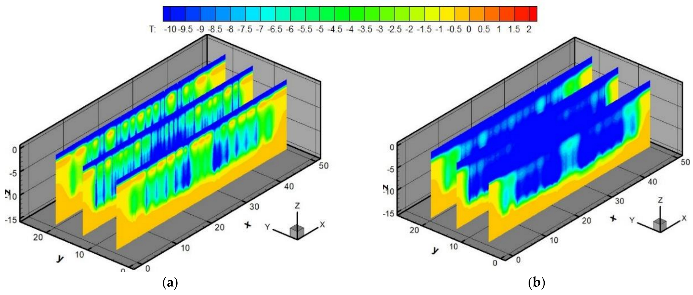
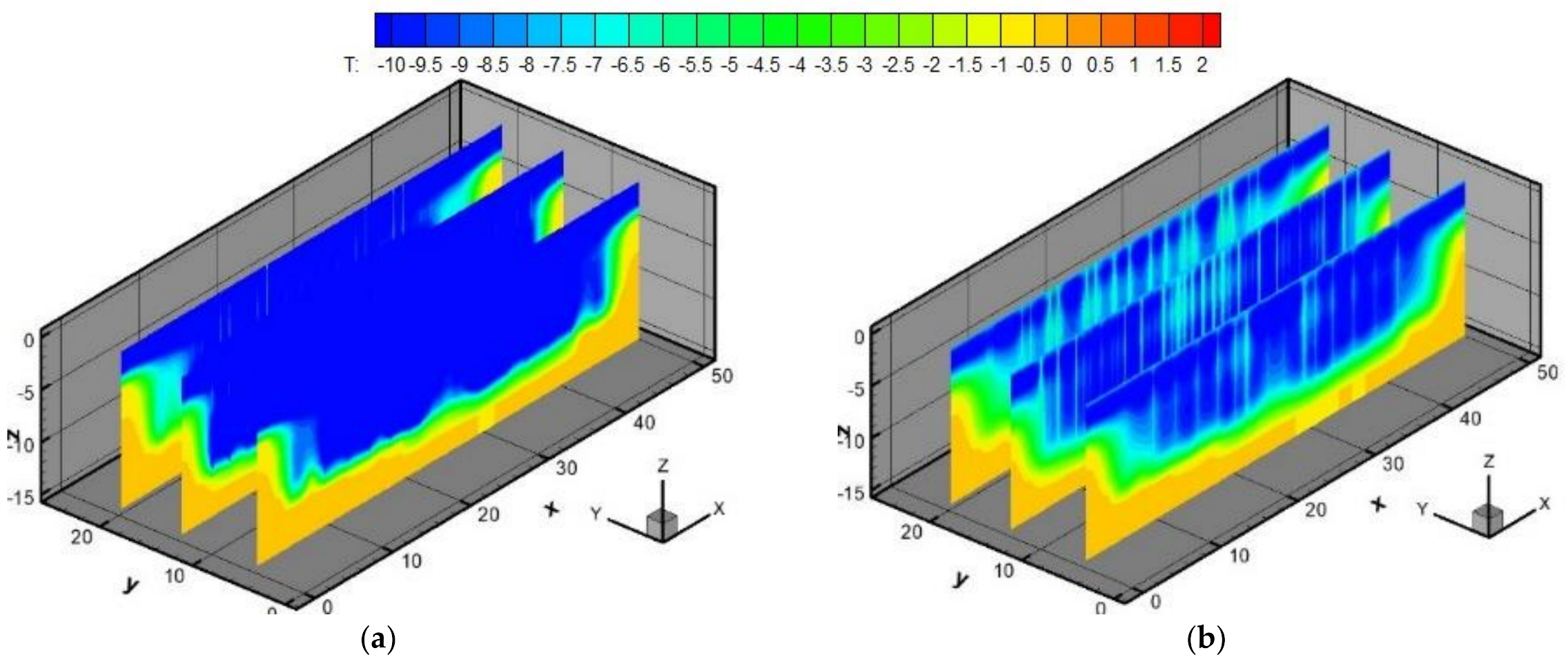
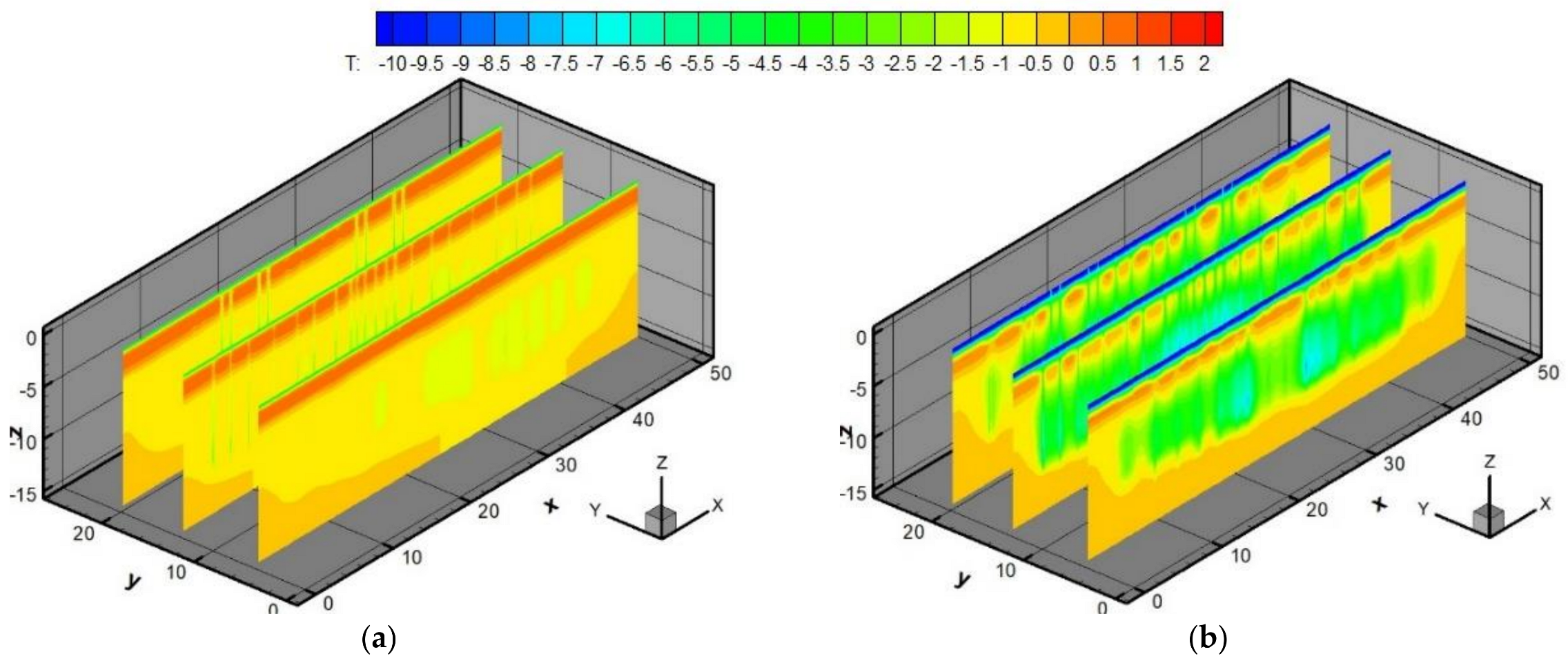
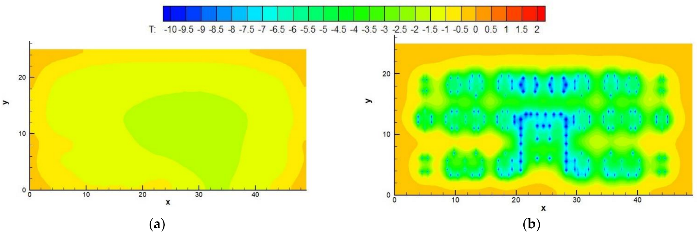
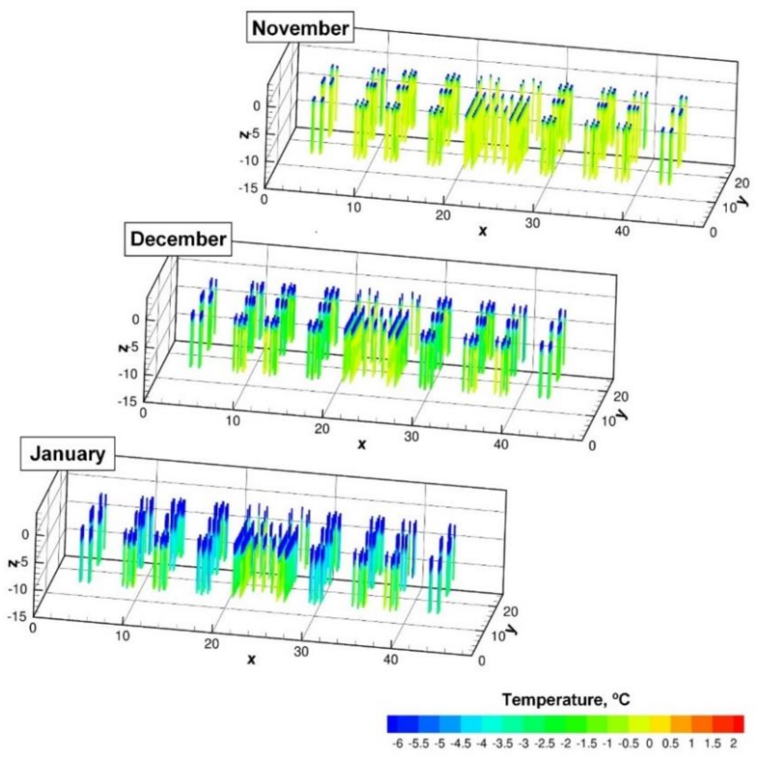
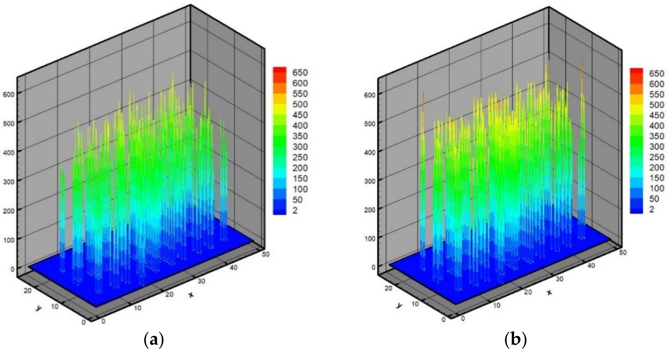
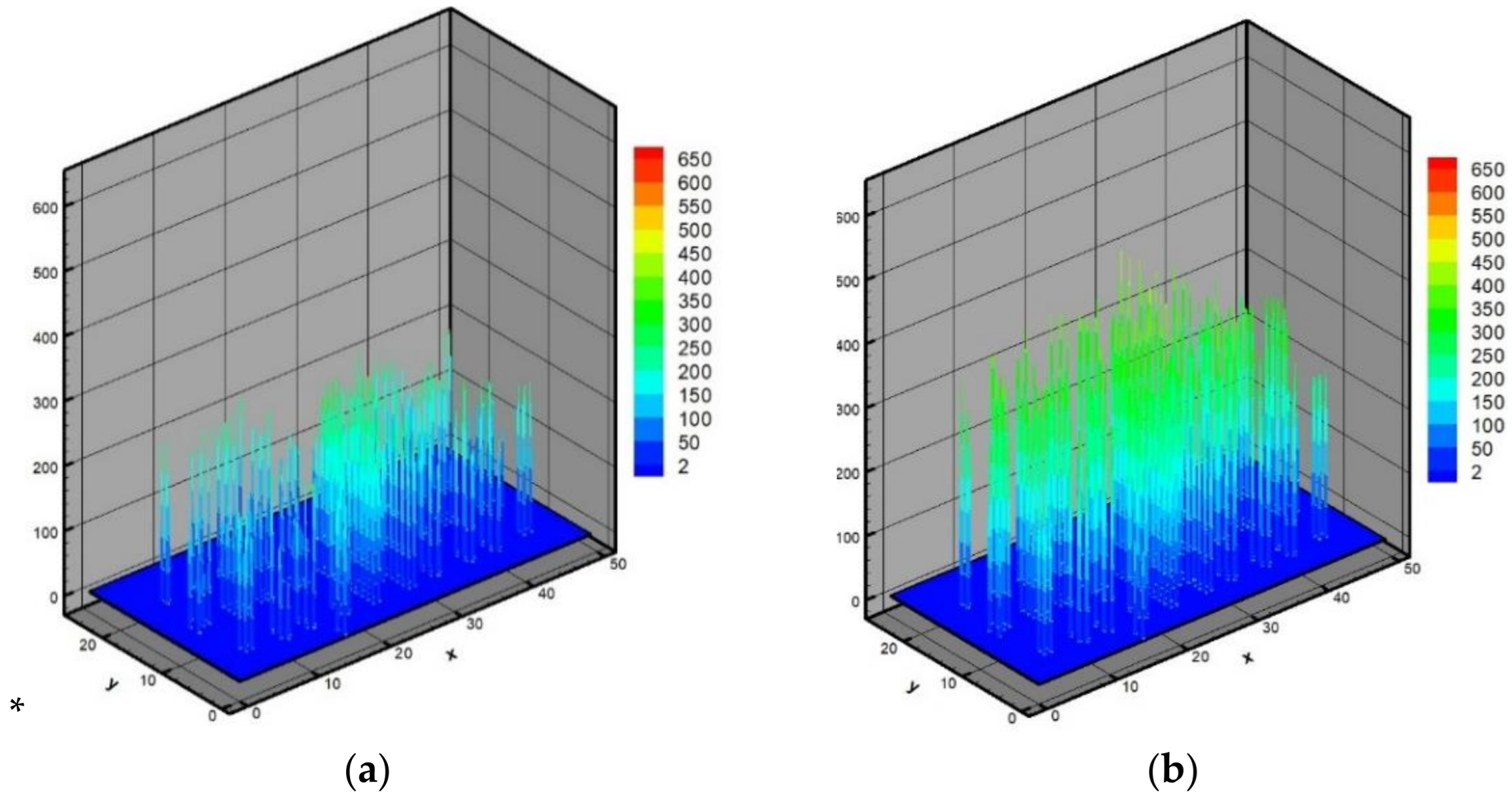
3.1. Temperature Fields in the Piling Foundation Area

Figure 4 shows the temperature field at the depth of 2.3 m in the {x, y} plane. The work of SCDs to cool the soil is clearly visible, intensifying in January. The warm area of the soil identified by thermometric wells begins to cool during the operation of the SCDs, which corresponds to further monitoring of the soil temperature.

Figure 5 shows the temperature field up to the depth 15 m in the {x, z} planes in December 2020 and January 2021. The work of SCDs in cooling the ground is clearly visible: the cooled area increases (shades of blue). The vertical planes show the cold accumulation in the zones of SCDs concentration and the effect of the upper layers of the riprap thermal isolation. The figure demonstrates the two main cold sources in the area: the upper active layer freezing and the effect of the SCDs operation in the deep of the zone. These zones merge and conserve the permafrost.

In these numerical experiments, we used daily average temperatures based on temperature monitoring data. In February, further cooling of the soil occurs, and the permafrost becomes continuous in the zone of PF with the SCDs supplementation, in contrast to the boundaries of the area, where only the upper layer is frozen. In March, the air temperature became greater than the temperature in the soil and the SCDs stop operating. A soil temperature increase is observed in Figure 6. In the summer period, further soil temperature increases have continued until October. In October, we can see the residual thermal traces of the SCDs working. In November, the soil cooling begins when SCDs start to work (Figure 7). In the {x, y} plane at the depth of 2.3 m, the temperature fields are shown in Figure 8 for comparing the September and November thermal fields. The cooler spot under the building is observed in the center of the zone; the boundaries of the foundation are weaker.

3.2. The Results of the Calculation of the Bearing Capacity of the Soil under Building I

To calculate the bearing capacity of the foundation piles, we find the temperature on the surface of the underground parts of the piles. Figure 9 shows the dynamics of temperature distribution on the pile surface for three months. After finding the temperature field in the PF zone, a two-dimensional horizontal uniform auxiliary grid is built in the {x, y} plane. At the nodes of this grid, the temperature distribution along the vertical dimension of the pile is determined. The auxiliar grid generates the dispersion of the bearing capacity that is due to the temperature difference in the different zones of the pile. For example, SCDs may be located nearer to one side of a pile, and the corresponding side will freeze stronger.

For each pile, we can determine the minimum and maximum bearing capacity values. To assess the bearing capacity of a pile [54], it is reasonable to use the minimum or average values obtained. If necessary, it is possible to calculate the contribution of each face to the bearing capacity of the pile.

The dynamics of changes in the bearing capacity of piles during the year from December to November is shown in Figure 10, Figure 11 and Figure 12. Note that 1 tf = 9806.65 N.

When designing a residential building, the minimum allowable parameters for the bearing capacity of piles are set, which must be observed during the operation of the building. These minimum values depend on the number of floors of the residential building, its size, and the type of piles. For a nine-story residential building, these parameters for piles should not be lower than 28.2 tf/m² or 53.8 tf/m² in dependence with the pile position.

The bearing capacity of the soil depends also on the temperature of the soil. By February, the soil is frozen not only because of the low air temperature and upper-layer freezing, but also because of the operation of SCDs. Therefore, the maximum bearing capacity of piles is reached by February. In the spring, when the air starts to warm up, the SCDs turn off and the soil begins to warm up. Therefore, the minimum bearing capacity of piles will be in September. Furthermore, the process of cooling and thawing of the soil is repeated. At the same time, one can notice an increase in the bearing capacity of the PF from the moment the building operation was started because of thermal stabilization of the soil using SCDs.

3.3. Validation of Numerical Calculations

To carry out numerical calculations in modeling thermal fields under Building I, the results of which are presented above, a refined grid was used (Figure 13). In the {x, y) plane, the number of grid nodes is 662 × 154 (grid 1).

To verify the numerical calculations, we will compare the results obtained for a sequence of refining grids. The annual mean of absolute differences are 0.68 °C for refined grid in (x, y) planes and 0.22 °C for refined grid in z axis in the considered vertical lines, corresponding to the SAM wells. Figure 14 shows the results of calculations on a denser grid compared to grid 1. The calculations performed show that the temperature profiles differ insignificantly over depth. Thus, the mesh size 331 × 154 × 16 = 815,584 nodes chosen for computer simulation can be used for calculations.

4. Discussion

To validate the numerical method, in addition to comparing the results on a sequence of the refined grids, it is also necessary to compare these results with the available data from 20 SAM wells 44–48 (Figure 1). In computer simulation of the problems (1)–(7), two approaches were used to set climatic parameters: in the ventilated underground, the average monthly temperature (AMT) of the air was set and, using temperature monitoring, the average daily temperature (ADT) was set. With the first approach, the calculated temperature profiles differed significantly from the temperature profiles in thermal wells. In Figure 15, the profiles of AMT and ADT of the air in the VU are shown during the observed year.

Figure 16 shows a comparison of numerical calculations using the AMT and ADT approaches with thermometry data for the SAM well 44–1 for various months. The better quantitative agreement of the obtained temperature profiles is reached for the ADT approach, and it was checked since refining the time step of 3 h does not give better results along the temperature setting every 3 h as the thermometrical equipment allows. Thus, it is shown that when considering climatic parameters when conducting heat engineering calculations, it is advisable to use the average daily air temperature.

Figure 17 shows the temperature distribution profiles in well 44–1 measured using temperature sensors (a) and obtained by numerical calculations (b). The model in Figure 17 used the average distribution temperature in November, obtained by the ATM system, as an initial condition (2). However, the thermometrical wells are located far enough from the SCDs zones and the initial temperature and the following temperature distribution, computed by the model, turned out warmer than the observed data in the winter and spring.

The operation of Building I began in October 2017, which means that it is necessary to consider the results of the work of SCDs on freezing the soil over several years of their operation with the respective thermal traces. The numerical calculations began in November 2020 and were based on current data from thermometric wells. At the same time, the prehistory of the functioning of 186 SCDs was not considered. Figure 18 shows a comparison of numerical calculations with thermometry data for well 44–1 for April and May 2021 after 1 year of operation of SCDs (continuous and dot lines).

Figure 18 shows a comparison of numerical calculations with thermometry data for well 44–1 for April and May 2021 after 3 years of operation of SCDs (continuous and dash lines).

Thus, the comparisons on Figure 18 indicate the need to consider the history of operation of the piling foundation and carry out calculations considering average daily temperatures based on temperature monitoring data when conducting thermal engineering calculations. The preliminary simulation of the history should be considered as the initial condition for the monitoring because the simplest average reconstruction of the data of thermometrical wells does not catch the local cold zones around SCDs.

Comparison of numerical calculations with thermometry data was carried out for all thermometrical wells. Figure 19 and Figure 20 compare temperatures in well 48–1 (see Figure 1) during 2021 for Building I. Calculated data and thermometry data are almost the same in summer and autumn (Figure 20). During this time the SCDs are not functional. In future work, it is planned to study in detail the effect of SCDs on the formation of temperature fields in the PF region.

An analysis of the PF areas in which the maximum differences between the calculated data and the thermometry data are observed showed that in these places there may be additional heat sources associated, for example, with the presence of heating networks.

The developed software based on the proposed model, which considers ATM data, makes it possible to assess changes in the bearing capacity of the soil under various scenarios of climate change. Figure 21 shows a short-term forecast of the change in the bearing capacity of piles under Building I for 2022.

In the future, it is planned to consider possible frost heaving. The studies presented in this article started a few years after the operation of this residential building; therefore, the essential stabilization processes associated, in particular, with shrinkage and other circumstances are in general completed and the further operation of the residential building will be determined by the temperature regime of the soils in the area of the PF. At present, according to the authors, SCD thermal stabilizers have a significant impact on the temperature regime of the soil. This is also confirmed by comparing the numerical results of temperatures in the SAM wells with temperature monitoring data. These results match very well during the summer when the SCDs are off. The greatest difference between the calculated data and monitoring data in some wells is observed in winter, when 186 SCDs work as the points of freezing in the soil. Therefore, it is important to use three-dimensional mathematical models and to approve the simulation of the operation of SCDs, the efficiency of which depends on the temperature difference in the ventilated underground and the ground temperature. Effectiveness of SCDs depends on the air temperature and it will be valuable to compare the results of the presented and models of the coupling between water and heat transfer [72,73,74,75,76,77,78,79,80].

5. Conclusions

• A new model and software are proposed for finding nonstationary thermal fields under Building I in the city of Salekhard, considering the data of thermometric observations from 20 thermometric wells that are sent to the server in real time.
• The developed software was validated and calibrated for the specific characteristics of the piling foundation (geometric arrangement of piles, seasonal cooling devices, locations of thermometric wells, and soil lithology).
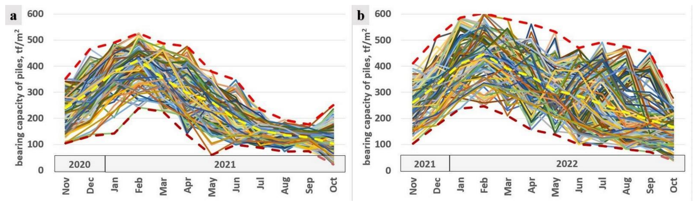
• This building’s designed load for one pile is from 28.2 tf/m² to 53.8 tf/m². The numerical results in Figure 21 show that by decreasing the temperature of soil of the PF by using SCDs thermal stabilizers, the bearing capacities of the piles increase over time and are also kept in the specified design values.
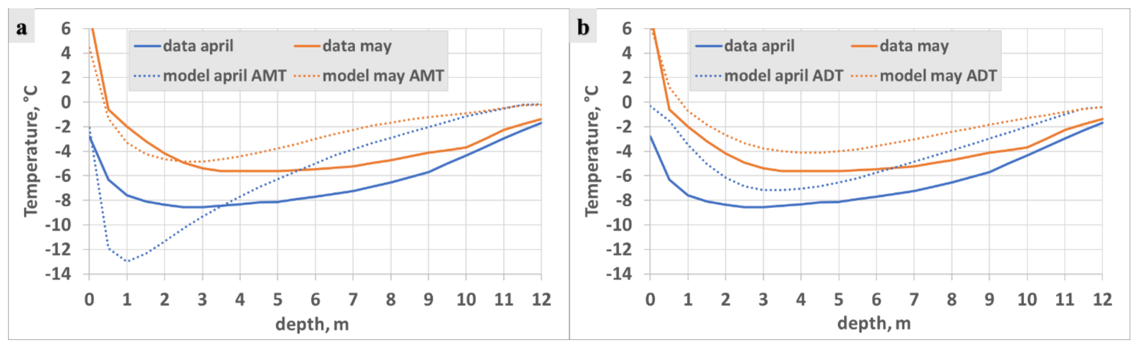
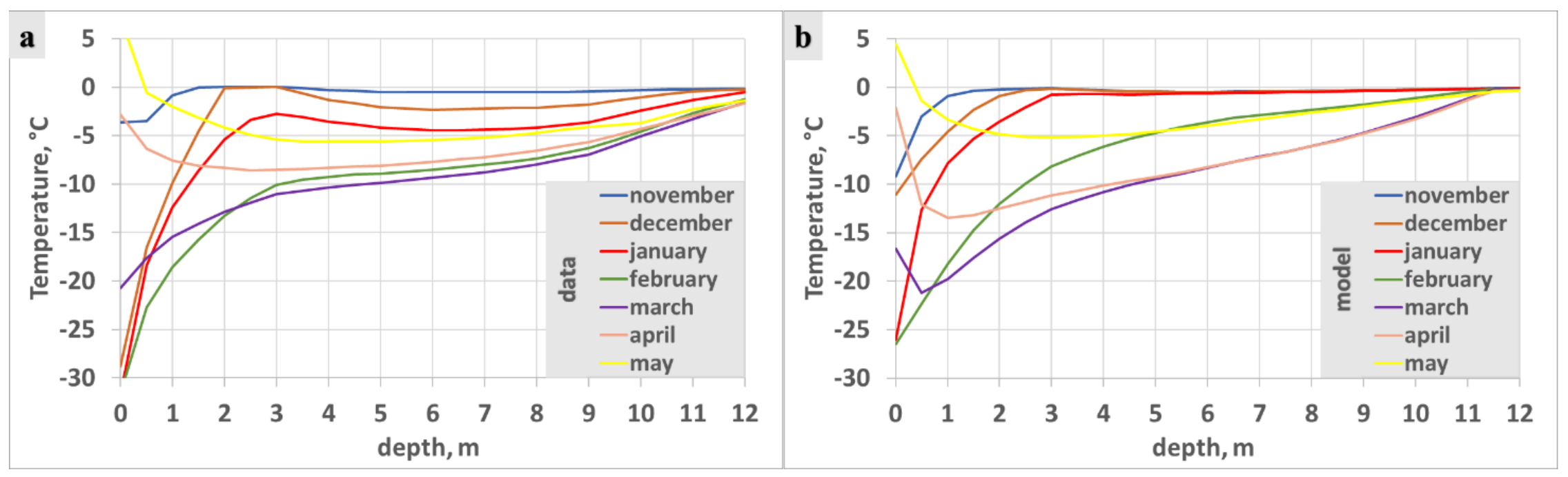
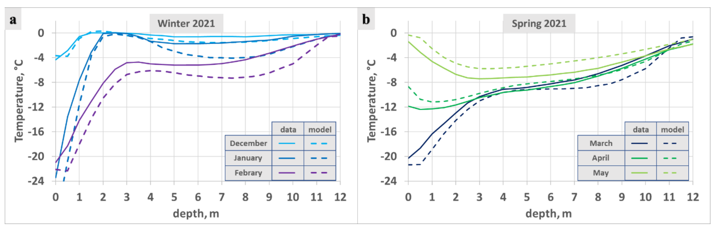
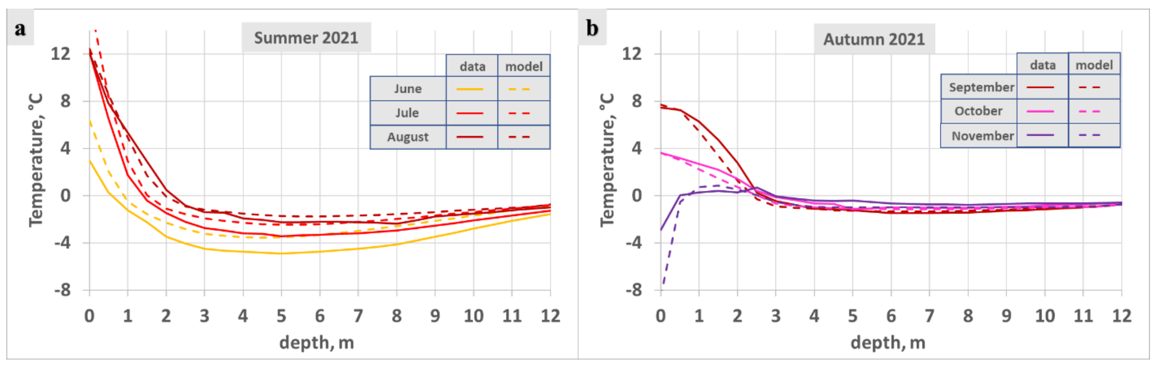
• Comparison of the thermometry data for the wells with the calculated data showed a good agreement in the summer and autumn periods. The difference between the thermometry data and the data obtained using computer simulation indicates the presence of additional heat sources, such as, for example, the presence of heat networks.
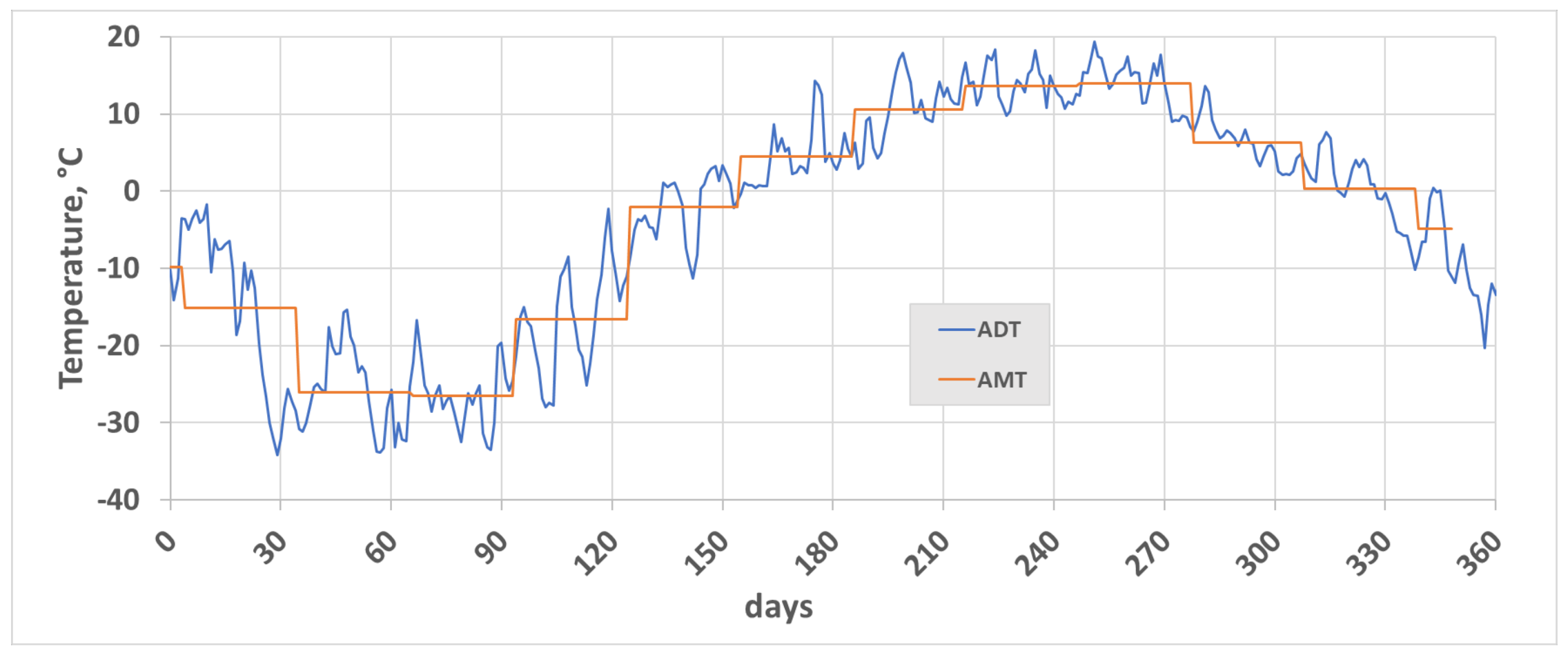
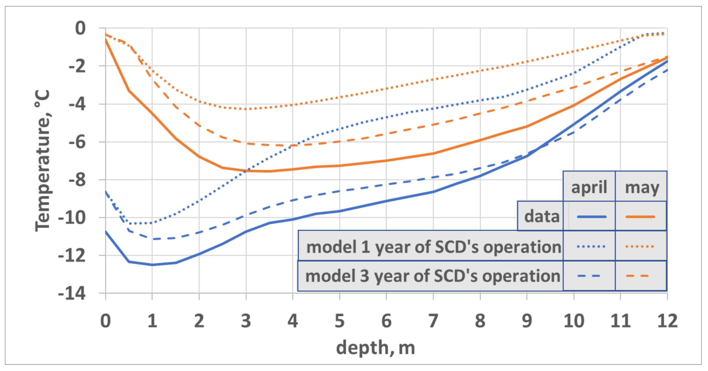
• In computer modeling, it is necessary to use the average daily temperature obtained as a result of temperature monitoring or a set, taking into account predicted climate changes. The accuracy of obtaining numerical results is also affected by the setting of the initial temperature distribution in the soil. For Building I, it was shown that it is necessary to consider at least three previous years of operation of seasonally operating devices around the piling foundation.
• The calculations for Building I indicate the bearing capacity of piles increases over time because of seasonal freezing of the soil.
• The combination of temperature monitoring methods with mathematical modeling methods makes it possible to create a digital model of a piling foundation and study changes in its various characteristics throughout the entire life of Building I. In the case of a predicted decrease in the bearing capacity of individual piles below the design values, it is necessary to use methods for thermal stabilization of the soil.
• The proposed method, which uses the data of a network of thermometric wells, can also be used for other construction projects with piling foundations in the permafrost zone.

References

1. Obu, J.; Westermann, S.; Bartsch, A.; Berdnikov, N.; Christiansen, H.H.; Dashtseren, A.; Delaloye, R.; Elberling, B.; Etzelmüller, B.; Kholodov, A.; et al. Northern Hemisphere permafrost map based on TTOP modelling for 2000–2016 at 1 km2 scale. Earth-Sci. Rev. 2019, 193, 136–155. [Google Scholar] [CrossRef]
2. Romanovsky, V.E.; Drozdov, D.S.; Oberman, N.G.; Malkova, G.V.; Kholodov, A.L.; Marchenko, S.S.; Moskalenko, N.G.; Sergeev, D.O.; Ukraintseva, N.G.; Abramov, A.; et al. Thermal state of permafrost in Russia. Permafr. Periglac. Process. 2010, 21, 136–155. [Google Scholar] [CrossRef]
3. Hassol, S.J. ACIA, Impacts of a Warming Arctic: Arctic Climate Impact Assessment; Cambridge University Press: Cambridge, UK, 2004; pp. 28–44. Available online: https://www.amap.no/documents/doc/impacts-of-a-warming-arctic-2004/786 (accessed on 19 March 2021).
4. Nelson, F.E.; Outcalt, S.I. A computational method for prediction and regionalization of permafrost. Arct. Alp. Res. 1987, 3, 279–288. [Google Scholar] [CrossRef]
5. Anisimov, O.A.; Nelson, F.E. Application of mathematical models to investigate the interaction between the climate and permafrost. Sov. Meteorol. Hydrol. 1990, 10, 8–13. [Google Scholar]
6. Daanen, R.P.; Ingeman-Nielsen, T.; Marchenko, S.S.; Romanovsky, V.E.; Foged, N.; Stendel, M.; Christensen, J.H.; Svendsen, K.H. Permafrost degradation risk zone assessment using simulation models. Cryosphere 2011, 5, 1043–1056. [Google Scholar] [CrossRef] [Green Version]
7. Jafarov, E.E.; Marchenko, S.S.; Romanovsky, V.E. Numerical modeling of permafrost dynamics in Alaska using a high spatial resolution dataset. Cryosphere 2012, 6, 613–624. [Google Scholar] [CrossRef] [Green Version]
8. Westermann, S.; Langer, M.; Boike, J.; Heikenfeld, M.; Peter, M.; Etzelmüller, B.; Krinner, G. Simulating the thermal regime and thaw processes of ice-rich permafrost ground with the land-surface model CryoGrid 3. Geosci. Model Dev. 2016, 9, 523–546. [Google Scholar] [CrossRef] [Green Version]
9. Filimonov, M.; Vaganova, N. Numerical Simulation of Technogenic and Climatic Influence on Permafrost. In Book Environmental Research; Daniels, J.A., Ed.; Nova Science Publishers: Hauppauge, NY, USA, 2017; Volume 54, pp. 117–142. [Google Scholar]
10. Rasmussen, L.H.; Zhang, W.; Hollesen, J.; Cable, S.; Christiansen, H.H.; Jansson, P.-E.; Bo, E. Modelling present and future permafrost thermal regimes in Northeast Greenland. Cold Reg. Sci. Technol. 2018, 146, 199–213. [Google Scholar] [CrossRef]
11. Streletskiy, D.A.; Shiklomanov, N.I.; Nelson, F.E. Spatial variability of permafrost active-layer thickness under contemporary and projected climate in northern Alaska. Polar Geogr. 2012, 35, 95–116. [Google Scholar] [CrossRef]
12. Peng, X.; Zhang, T.; Frauenfeld, O.W.; Kang, W.; Luo, D.; Cao, B.; Hang, S.; Jin, H.; Wu, Q. Spatiotemporal changes in active layer thickness under contemporary and projected climate in the northern hemisphere. J. Clim. 2018, 31, 251–266. [Google Scholar] [CrossRef]
13. Peng, X.; Zhang, T.; Frauenfeld, O.W.; Du, R.; Wei, Q.; Liang, B. Soil freeze depth variability across Eurasia during 1850–2100. Clim. Chang. 2020, 158, 531–549. [Google Scholar] [CrossRef]
14. Shestakova, A.A.; Fedorov, A.N.; Torgovkin, Y.I.; Konstantinov, P.Y.; Vasyliev, N.F.; Kalinicheva, S.V.; Samsonova, V.V.; Hiyama, T.; Iijima, Y.; Park, H.; et al. Mapping the Main Characteristics of Permafrost on the Basis of a Permafrost-Landscape Map of Yakutia Using GIS. Land 2021, 10, 462. [Google Scholar] [CrossRef]
15. Vasiliev, A.A.; Drozdov, D.S.; Gravis, A.G.; Nikitin, K.A. Permafrost degradation in YANAO. Results of the long-term monitoring. In Proceedings of the International Conference “Modern Studies of Cryosphere Transformation and Geotechnical Safety Issues for Construction in the Arctic, 2021”, Salekhard, Russia, 8–12 November 2021. [Google Scholar]
16. Nelson, F.E.; Anisimov, O.A.; Shiklomanov, N.I. Subsidence risk from thawing permafrost. Nature 2001, 410, 889–890. [Google Scholar] [CrossRef]
17. Pepin, N.; Bradley, R.S.; Diaz, H.F.; Baraer, M.; Caceres, E.B.; Forsythe, N.; Fowler, H.; Greenwood, G.; Hashmi, M.Z.; Liu, X.D.; et al. Elevation-dependent warming in mountain regions of the world. Nat. Clim. Chang. 2015, 5, 424–430. [Google Scholar] [CrossRef]
18. Guo, D.; Wang, H. CMIP5 permafrost degradation projection: A comparison among different regions. J. Geophys. Res. Atmos. 2016, 121, 4499–4517. [Google Scholar] [CrossRef]
19. Guo, D.; Wang, H. Permafrost degradation and associated ground settlement estimation under 2 °C global warming. Clim. Dyn. 2017, 49, 2569–2583. [Google Scholar] [CrossRef]
20. Chadburn, S.E.; Burke, E.J.; Cox, P.M.; Friedlingstein, P.; Hugelius, G.; Westermann, S. An observation-based constraint on permafrost loss as a function of global warming. Nat. Clim. Chang. 2017, 7, 340–344. [Google Scholar] [CrossRef]
21. Wang, K.; Zhang, T.; Zhang, X.; Gray, C.; Jafarov, E.; Overeem, I.; Romanovsky, V.; Peng, X.; Cao, B. Continuously amplified warming in the Alaskan Arctic: Implications for estimating global warming hiatus. Geophys. Res. Lett. 2017, 44, 9029–9038. [Google Scholar] [CrossRef]
22. Vasiliev, A.A.; Drozdov, D.S.; Gravis, A.G.; Malkova, G.V.; Nyland, K.E.; Streletskiy, D.A. Permafrost degradation in the Western Russian Arctic. Environ. Res. Lett. 2020, 15, 045001. [Google Scholar] [CrossRef]
23. Alexandrov, G.A.; Ginzburg, V.A.; Insarov, G.E.; Romanovskaya, A.A. CMIP6 model projections leave no room for permafrost to persist in Western Siberia under the SSP5-8.5 scenario. Clim. Chang. 2021, 169, 42. [Google Scholar] [CrossRef]
24. Biskaborn, B.K.; Smith, S.L.; Noetzli, J.; Matthes, H.; Vieira, G.; Streletskiy, D.A.; Schoeneich, P.; Romanovsky, V.E.; Lewkowicz, A.G.; Abramov, A.; et al. Permafrandost is warming at a global scale. Nat. Commun. 2019, 10, 264. [Google Scholar] [CrossRef] [Green Version]
25. Filimonov, M.Y.; Vaganova, N.A. Simulation of technogenic and climatic influences in permafrost for northern oil fields exploitation. In Finite Difference Methods, Theory and Applications. FDM 2014. Lecture Notes in Computer Science; Springer: Cham, Switzerland, 2015; Volume 9045, pp. 185–192. [Google Scholar] [CrossRef]
26. Vaganova, N.; Filimonov, M.Y. Different shapes of constructions and their effects on permafrost. AIP Conf. Proc. 2016, 1789, 020019. [Google Scholar] [CrossRef]
27. Wu, Q.; Zhang, Z.; Gao, S.; Ma, W. Thermal impacts of engineering activities on permafrost in different alpine ecosystems in Qinghai-Tibet plateau, China. Cryosphere 2016, 10, 1695–1706. [Google Scholar] [CrossRef] [Green Version]
28. Filimonov, M.; Vaganova, N. Permafrost thawing from different technical systems in Arctic regions. IOP Conf. Ser. Earth Environ. Sci. 2017, 72, 012006. [Google Scholar] [CrossRef] [Green Version]
29. Gladkikh, V.S.; Ilin, V.P.; Petukhov, A.V.; Krylov, A.M. Numerical modeling of non-stationary heat problems in a two-phase medium. J. Phys. Conf. Ser. 2021, 1715, 012002. [Google Scholar] [CrossRef]
30. Streletskiy, D.A.; Shiklomanov, N.I.; Grebenets, V.I. Changes of foundation bearing capacity due to climate warming in Northwest Siberia. Earth Cryosphere 2012, 16, 22–32. (In Russian) [Google Scholar]
31. Shiklomanov, N.I.; Streletskiy, D.A.; Swales, T.B.; Kokorev, V.A. Climate change and stability of urban infrastructure in Russian permafrost regions: Prognostic assessment based on GCM climate projections. Geogr. Rev. 2017, 107, 125–142. [Google Scholar] [CrossRef]
32. Hjort, J.; Karjalainen, O.; Aalto, J.; Westermann, S.; Romanovsky, V.E.; Nelson, F.E.; Etzelmüller, B.; Luoto, M. Degrading permafrost puts Arctic infrastructure at risk by mid-century. Nat. Commun. 2018, 9, 5147. [Google Scholar] [CrossRef]
33. Suter, L.; Streletskiy, D.; Shiklomanov, N. Assessment of the cost of climate change impacts on critical infrastructure in the circumpolar Arctic. Polar Geogr. 2019, 42, 267–286. [Google Scholar] [CrossRef]
34. Schneider von Deimling, T.; Ingeman-Nielsen, T.; Lee, H.; Westermann, S. Modelling consequences of permafrost degradation for Arctic infrastructure and related risks to the environment and society. In Proceedings of the Arctic Science Summit Week 2021, Lisbon, Portugal, 20–26 March 2021; Available online: https://orbit.dtu.dk/en/publications/modelling-consequences-of-permafrost-degradation-for-arctic-infra (accessed on 19 March 2021).
35. Amosova, E.V.; Kropachev, D.Y.; Pazderin, D.S. Temperature monitoring system for extended objects in permafrost. Equip. Technol. Oil Gas Complex 2011, 2, 67–70. [Google Scholar]
36. Vaganova, N.; Filimonov, M. Simulation of freezing and thawing of soil in Arctic regions. IOP Conf. Ser. Earth Environ. 2017, 72, 012006. [Google Scholar] [CrossRef] [Green Version]
37. Streletskiy, D.A.; Suter, L.J.; Shiklomanov, N.I.; Porfiriev, B.N.; Eliseev, D.O. Assessment of climate change impacts on buildings, structures and infrastructure in the Russian regions on permafrost. Environ. Res. Lett. 2019, 14, 025003. [Google Scholar] [CrossRef]
38. Smith, S.L.; Burgess, M.M.; Riseborough, D.; Nixon, F.M. Recent Trends from Canadian Permafrost Thermal Monitoring Network Sites. Permafr. Periglac. Process. 2005, 16, 19–30. [Google Scholar] [CrossRef]
39. Yeltsov, I.N.; Olenchenko, V.V.; Faguet, A.N. Electrotomography in the Russian Arctic based on field studies and three-dimensional numerical modeling. Bus. Mag. Neftegaz. RU 2017, 2, 54–64. (In Russian) [Google Scholar]
40. You, Y.; Yu, Q.; Pan, X.; Wang, X.; Guo, L. Application of electrical resistivity tomography in investigating depth of permafrost base and permafrost structure in Tibetan Plateau. Cold Reg. Sci. Technol. 2013, 87, 19–26. [Google Scholar] [CrossRef]
41. Gryaznova, E. Geotechnical monitoring to ensure reliability of construction and operation of buildings and structures. IOP Conf. Ser. Mater. Sci. Eng. 2018, 365, 052014. [Google Scholar] [CrossRef] [Green Version]
42. Gromadsky, A.N.; Arefiev, S.V.; Volkov, N.G.; Kamnev, Y.K.; Sinitsky, A.I. Remote monitoring of the temperature regime of permafrost soils under the buildings of Salekhard. Sci. Bull. Yamalo-Nenets Auton. Okrug 2019, 3, 17–21. [Google Scholar] [CrossRef]
43. Kamnev, Y.K.; Filimonov, M.Y.; Shein, A.N.; Vaganova, N.A. Automated Monitoring the Temperature Under Buildings with Pile Foundations in Salekhard (Preliminary Results). Geogr. Environ. Sustain. 2021, 14, 75–82. [Google Scholar] [CrossRef]
44. Potapov, A.I.; Shikhov, A.I.; Dunaeva, E.N. Geotechnical monitoring of frozen soils: Problems and possible solutions. IOP Conf. Ser. Mater. Sci. Eng. 2021, 1064, 012038. [Google Scholar] [CrossRef]
45. Varlamov, S.P.; Skachkov, Y.B.; Skryabin, P.N. Long-Term Variability in Ground Thermal State in Central Yakutia’s Tuymaada Valley. Land 2021, 10, 1231. [Google Scholar] [CrossRef]
46. Bouffard, T.J.; Uryupova, E.; Dodds, K.; Romanovsky, V.E.; Bennett, A.P.; Streletskiy, D. Scientific Cooperation: Supporting Circumpolar Permafrost Monitoring and Data Sharing. Land 2021, 10, 590. [Google Scholar] [CrossRef]
47. Alekseev, A.; Shilova, L.; Mefedov, E. An approach for automatization of geotechnical monitoring in cryolithozone. IOP Conf. Ser. Mater. Sci. Eng. 2021, 1083, 012080. [Google Scholar] [CrossRef]
48. System of Automated Geocryological Monitoring. Available online: https://monitoring.arctic.yanao.ru/ (accessed on 15 February 2021).
49. Ishkov, A.; Anikin, G.V.; Dolgikh, G.M.; Okunev, S.N. Horizontal evaporator tube (HET) thermosyphons: Physicalmathematical modeling and experimental data, compared. Earth’s Cryosphere 2018, 22, 57–64. (In Russian) [Google Scholar]
50. Baisheva, L.M.; Permyakov, P.P.; Bolshakov, A.M. Heat and Mass Transfer of a Coolant in Horizontal Seasonal Cooling Devices. IOP Conf. Ser. Mater. Sci. Eng. 2020, 753, 042092. [Google Scholar] [CrossRef]
51. Filimonov, M.Y.; Vaganova, N.A. Simulation of thermal stabilization of soil around various technical systems operating in permafrost. Appl. Math. Sci. 2013, 7, 7151–7160. [Google Scholar] [CrossRef]
52. Perreault, P.; Shur, Y. Seasonal thermal insulation to mitigate climate change impacts on foundations in permafrost regions. Cold Reg. Sci. Technol. 2016, 132, 7–18. [Google Scholar] [CrossRef]
53. Harlan, R.; Nixon, J. Ground Thermal Regime. Geotechnical Engineering for Cold Regions; Andersland, O.B., Anderson, D.M., Eds.; McGraw-Hill: New York, NY, USA, 1978; pp. 103–163. [Google Scholar]
54. SP 25.13330.2021; Soil Bases and Foundations on Permafrost Soils. The Federal Agency for Technical Regulation and Metrology (Rosstandart): Moscow, Russia, 2021. (In Russian)
55. Pustovoit, G.P. On the potential of seasonal in-ground cooling devices. Soil Mech. Found. Eng. 2015, 42, 142–146. [Google Scholar] [CrossRef]
56. Vaganova, N.A. Simulation of Thermal Stabilization of Bases under Engineering Structures in Permafrost Zone. AIP Conf. Proc. 2018, 2048, 030010. [Google Scholar] [CrossRef] [Green Version]
57. Vaganova, N.A.; Filimonov, M.Y. Simulation of Cooling Devices and Effect for Thermal Stabilization of Soil in a Cryolithozone with Anthropogenic Impact. In Finite Difference Methods, Theory and Applications. FDM 2014. Lecture Notes in Computer Science; Springer: Cham, Switzerland, 2019; Volume 11386, pp. 580–587. [Google Scholar] [CrossRef]
58. Gorelik, J.B.; Khabitov, A.K.; Zemerov, I.V. Affectivity of surface cooling of the building’s bases on permafrost. In Proceedings of the International Conference “Modern Studies of Cryosphere Transformation and Geotechnical Safety Issues for Construction in the Arctic, 2021”, Salekhard, Russia, 8–12 November 2021. [Google Scholar]
59. Okorokov, N.S.; Korkishko, A.N.; Korzhikova, A.P. An experimental study of a forced ventilation pile. Vestnik MGSU 2020, 15, 665–677. [Google Scholar] [CrossRef]
60. Klimov, A.S.; Emelyanov, R.T.; Chumakova, E.V.; Klimova, O.L. Cooling of near-pile permafrost soils in the arctic region. J. Constr. Archit. 2021, 23, 138–146. (In Russian) [Google Scholar] [CrossRef]
61. Filimonov, M.Y.; Vaganova, N.A. Thawing of Permafrost During the Operation of Wells of North-Mukerkamyl Oil and Gas Field. J. Sib. Fed. Univ. Math. Phys. 2021, 14, 795–804. [Google Scholar] [CrossRef]
62. Alekseeva, M.N.; Yashchenko, I.G. Ecological Aspects of Hydrocarbon Extraction in the Purovsky Region of Yamalo-Nenets Autonomous District. Chem. Sustain. Dev. 2021, 29, 116–122. [Google Scholar] [CrossRef]
63. Samarskii, A.A.; Moiseyenko, B.D. An economic continuous calculation scheme for the Stefan multidimensional problem. USSR Comput. Math. Math. Phys. 1965, 5, 43–58. Available online: http://samarskii.ru/articles/1965/1965-002.pdf (accessed on 19 March 2021). [CrossRef]
64. Samarsky, A.A.; Vabishchevich, P.N. Computational Heat Transfer, Volume 2, the Finite Difference Methodology; Wiley: Chichester, UK, 1995. [Google Scholar]
65. Walvoord, M.A.; Kurylyk, B.L. Hydrologic impacts of thawing permafrost—A review. Vadose Zone J. 2016, 15. [Google Scholar] [CrossRef]
66. Grenier, C.; Anbergen, H.; Bense, V.; Chanzy, Q.; Coon, E.; Collier, N.; Costard, F.; Ferry, M.; Frampton, A.; Frederick, J.; et al. Groundwater flow and heat transport for systems undergoing freeze-thaw: Intercomparison of numerical simulators for 2D test cases. Adv. Water Resour. 2018, 114, 196–218. [Google Scholar] [CrossRef]
67. Lamontagne-Hallé, P.; McKenzie, J.M.; Molson, J.; Lyon, B.L.; Kurylyk, L.N. Guidelines for cold-regions groundwater numerical modeling. WIREs Water 2020, 7, e1467. [Google Scholar] [CrossRef]
68. Yang, X.; Hu, J.; Ma, R.; Sun, Z. Integrated Hydrologic Modelling of Groundwater-Surface Water Interactions in Cold Regions. Front. Earth Sci. 2021, 9, 721009. [Google Scholar] [CrossRef]
69. Hinkel, K.M.; Outcalt, S.I.; Taylor, A.E. Seasonal patterns of coupled flow in the active layer at three sites in northwest North America. Can. J. Earth Sci. 1997, 34, 667–678. [Google Scholar] [CrossRef]
70. Kane, D.L.; Hinkel, K.M.; Goering, D.J.; Hinzman, L.D.; Outcalt, S.I. Non-conductive heat transfer associated with frozen soils. Glob. Planet. Chang. 2001, 29, 275–292. [Google Scholar] [CrossRef]
71. Zhirkov, A.; Permyakov, P.; Wen, Z.; Kirillin, A. Influence of Rainfall Changes on the Temperature Regime of Permafrost in Central Yakutia. Land 2021, 10, 1230. [Google Scholar] [CrossRef]
72. Filimonov, M.Y.; Vaganova, N.A. On Boundary Conditions Setting for Numerical Simulation of Thermal Fields Propagation in Permafrost Soils. CEUR-WS Proc. 2018, 2109, 18–24. Available online: http://ceur-ws.org/Vol-2109/paper-04.pdf (accessed on 14 July 2022).
73. Huang, X.; Rudolph, D.L. A hybrid analytical-numerical technique for solving soil temperature during the freezing process. Adv. Water Resour. 2022, 162, 104163. [Google Scholar] [CrossRef]
74. Kurylyk, B.L.; Watanabe, K. The mathematical representation of freezing and thawing processes in variably-saturated, non-deformable soils. Adv. Water Resour. 2013, 60, 160–177. [Google Scholar] [CrossRef]
75. Kurylyk, B.L.; Hayashi, M.; Quinton, W.L.; McKenzie, J.M.; Voss, C.I. Influence of vertical and lateral heat transfer on permafrost thaw, peatland landscape transition, and groundwater flow. Water Resour. Res. 2016, 52, 1286–1305. [Google Scholar] [CrossRef] [Green Version]
76. Magnússon, R.Í.; Hamm, A.; Karsanaev, S.V.; Limpens, J.; Kleijn, D.; Frampton, A.; Maximov, T.C.; Heijmans, M.M.P.D. Extremely wet summer events enhance permafrost thaw for multiple years in Siberian tundra. Nat. Commun. 2022, 13, 1556. [Google Scholar] [CrossRef]
77. Painter, S.L.; Karra, S. Constitutive model for unfrozen water content in subfreezing unsaturated soils. Vadose Zone J. 2014, 13, 1–8. [Google Scholar] [CrossRef]
78. Sjöberg, Y.; Coon, E.; Sannel, A.B.K.; Pannetier, R.; Harp, D.; Frampton, A.; Painter, S.L.; Lyon, S.W. Thermal effects of groundwater flow through subarctic fens: A case study based on field observations and numerical modeling. Water Resour. Res. 2016, 52, 1591–1606. [Google Scholar] [CrossRef] [Green Version]
79. Orgogozo, L.; Prokushkin, A.S.; Pokrovsky, O.S.; Grenier, C.; Quintard, M.; Viers, J.; Audry, S. Water and energy transfer modelling in a permafrost-dominated, forested catchment of Central Siberia: The key role of rooting depth. Permafr. Periglac. Process. 2019, 30, 75–89. [Google Scholar] [CrossRef]
80. Zipper, S.C.; Lamontagne-Hallé, P.; McKenzie, J.M.; Rocha, A.V. Groundwater controls on postfire permafrost thaw: Water and energy balance effects. J. Geophys. Res. Earth Surf. 2018, 123, 2677–2694. [Google Scholar] [CrossRef]
81. Vaganova, N.A. Existence of a solution of an initial-boundary value difference problem for a linear heat equation with a nonlinear boundary condition. Proc. Steklov Inst. Math. 2008, 261 (Suppl. 1), S260–S271. [Google Scholar] [CrossRef]
Figure 1. Scheme of the location of thermometric equipment of the SAMs and the PF under Building I. The triangles are the SAM wells, the squares are the SAM stations, and the dots are the piles.
Land 11 01102 g001
Figure 2. Soil structure in the area of the PF according to the soil numbers in Table 1.
Land 11 01102 g002
Figure 3. Scheme of the PF under Building I with the piles (red spots) and SCDs (blue spots).
Land 11 01102 g003
Figure 4. Temperature field at the depth of 2.3 m under Building I in December 2020 (a) and January 2021 (b) in the {x, y} plane.
Land 11 01102 g004
Figure 5. Temperature fields in the {x, z} plane under Building I in December 2020 (a) and January 2021 (b) in the vertical slices.
Land 11 01102 g005
Figure 6. Temperature fields in the {x, z} plane under Building I in February 2021 (a) and March 2021 (b) in the vertical slices.
Land 11 01102 g006
Figure 7. Temperature fields in the {x, z} plane under Building I in October 2021 (a) and November 2021 (b) in the vertical slices.
Land 11 01102 g007
Figure 8. Temperature field at the depth of 2.3 m under Building I in September 2021 (a) and November 2021 (b) in the {x, y} plane.
Land 11 01102 g008
Figure 9. Temperature on the pile surfaces in November 2020, December 2020, and January 2021.
Land 11 01102 g009
Figure 10. Bearing capacity of piles in December 2020 (a) and in February 2021 (b) in tf/m2.
Land 11 01102 g010
Figure 11. Bearing capacity of piles in April 2021 (a) and in September 2021 (b) in tf/m2.
Land 11 01102 g011
Figure 12. Bearing capacity of piles in October 2021 (a) and in November 2021 (b) in tf/m2.
Land 11 01102 g012
Figure 13. Horizontal view of the computational grid in the {x, y} plane for Building I.
Land 11 01102 g013
Figure 14. Comparison of temperature profiles at a depth of up to 15 m, calculated on a grid of 331 × 154 × 16 and a two-times finer grid {x, y} on a grid of 662 × 154 × 16 (a) and on a grid of 331 × 154 × 39 (b).
Land 11 01102 g014
Figure 15. Average daily temperature (ADT) and average monthly temperatures (AMT) during the observation period.
Land 11 01102 g015
Figure 16. Temperature profiles calculated with average monthly temperatures—AMT (a), average daily temperature—ADT (b), in comparing with thermometry data for Building I.
Land 11 01102 g016
Figure 17. Dynamics of temperature change in well 44–1 in 2021 obtained from temperatures measured using temperature sensors (a) and numerical calculations (b).
Land 11 01102 g017
Figure 18. Temperature profiles in SAM well 44–1 in April–May 2021 obtained from temperatures measured using temperature sensors (continuous lines), numerical calculations which used 1 year of operation of SCDs (dot lines) and 3 years of operation of SCDs (dash lines).
Land 11 01102 g018
Figure 19. Comparison of temperature profiles in SAM well 48–1 in 2021 in winter (a) and spring (b).
Land 11 01102 g019
Figure 20. Comparison of temperature profiles in SAM well 48–1 in 2021 in summer (a) and autumn (b).
Land 11 01102 g020
Figure 21. Dynamics of change in the predicted change in the bearing capacity of piles in 2021 (a) in comparison with the obtained change in the bearing capacity of piles in 2022 (b) in tf/m2.
Land 11 01102 g021