1. Introduction
The current research is part of larger efforts to mainstream sustainability at sectoral levels. In this case, the perspective of decoupling economic development from resource inputs is bringing to the forefront the approach of reducing environmental impacts and climate change.
The patterns of consumption have a long-term trend that should be taken into account more when the decoupling process is looked at. According to [
1] (UNEP, 2021), more than 95% of all materials used throughout history came from biomass. Currently, there is a consensus that economic development should go in the direction of increasing the conservation of the limited natural resources of the planet and environmental protection. The process of transitioning towards sustainable development approaches (such as a circular economy, decoupling processes, bio-based products, etc.) are part of the implementation of the 2030 Agenda for Sustainable Development.
When it comes to implementing new approaches, the Ministerial Declaration elaborated on the High-Level Political Forum on Sustainable Development [
2] (HLPF 2018) states that ‘decoupling economic growth from use resources continue to be a challenge’. The effort towards a decoupling process is not easy, but necessarily serves as ‘preconditions for reducing poverty and social inequalities’ and ‘to delinking economic development from environmental deterioration’ [
3]. (UNEP, 2011).
At the European level, the multiple functions of forests are acknowledged through strategic natural protection policies, such as the EU Forestry Strategy for 2030 [
4] (European Commission, 2021) and the EU Biodiversity Strategy for 2030 [
5] (European Commission, 2020). As regards sustainability criteria, the EU Forest Strategy for 2030 mentions this option especially in the case of energy production. Furthermore, supporting afforestation projects is part of the solution to offset air pollution and to achieve the goal of climate neutrality.
The process of decarbonising the EU’s economy by 2050 also envisages the sustainable use of bioenergy as an alternative to fossil fuels. Along with this aim, there is a need to have criteria for sustainable forest management and for the protection of areas rich in biodiversity. All these new directions of action will have to ensure a better promotion of sustainability principles in relation to biomass, both solid and gaseous, for electricity production, heating, and cooling.
At the national level, the Recovery and Resilience Plan for Romania [
6] foresees a series of reforms and investments exclusively in the forestry sector (e.g., the adoption of the National Forest Strategy, the ecological reconstruction of habitats, the conservation of species, etc.). Furthermore, as a nexus regarding resource efficiency, material reuse and reducing waste, the Recovery and Resilience Plan states the aim to ensure Romania’s transition to a circular economy by 2030.
This paper emphasizes the relations existing between the triad represented by economic development, resource consumption and associated implications and challenges for the forested areas in Romania. In this regard, we have used both qualitative and quantitative methods, and the main hypothesis is the premise that decoupling is a process of using less resources per unit of economic output, this paper started to investigate the findings of the Environmental Kuznets Curve (EKC) and to propose an adaptation of the Kuznets Curve initially described by Kuznets (1955) [
7]. More specifically, it assumes that involves a direct link between certain indicators of environmental degradation and social well-being. Welfare is often measured either by per capita GDP or income. In the early stages of economic growth, environmental degradation and pollution will increase to an inflection point, but after a certain level of per capita income (influenced by various factors specific to the analyzed economy. This trend will be reversed towards a reduction in environmental degradation and pollution (Stern, 2003) [
8]. The change from Kuznets’ initial curve consists of replacing the order of social inequality with the one of the qualities of the environment.
There are a number of theoretical arguments that can support the reduction in environmental hazards through economic growth, as described by Van Alstine and Neumayer (2010) [
9]: (i) the quality of the environment is considered to be a public good; (ii) as economic growth takes place, the possibility of introducing new, more efficient and less polluting technologies will be increased; (iii) the increase in the share of services compared to the share of the industry in the total production and the intersectoral changes will lead to a decrease in pollution (Jänicke, Binder, & Mönch, 1997) [
10]; and (iv) the increase in income will lead to a decrease in the population growth rate, and the pressure on the environment by the population will be lower. Therefore, there are debates when it comes to the theoretical framework, and there is not a single model fitting all situations when it comes to the process of economic growth. In the second phase, as described by the Kuznets environment curve, it will not have always have a positive impact on the environment.
2. Materials and Methods
The Kuznets environmental curve is itself a theory based on an empirical factor, but the econometric models designed are not yet sufficiently developed to support this theory (Stern, 2003) [
8]. At the same time, Perman and Stern (2003) [
11] argue that these econometric models do not always consider the quality and homogeneity of the processed data nor the post-processing statistical tests that confirm the existence of false regressive models. Thus, the econometric models that test the environmental curve show still unclear results, noting the lack of consensus on the topic discussed in the literature.
In a significant number of studies, the Kuznets equation of the environmental curve is described according to:
where
E is the environmental variable,
Y expresses income or output per capita,
F refers to the country/economy specific effects and
k represents a dummy variable or an identified time trend.
Thus, if δ is negative and statistically significant and ∅ is insignificant, then we obtain scenario A. This scenario implies a reduction in the degree of environmental degradation as the income per capita increases over time.
If δ is positive and statistically significant and ∅ is insignificant, then we will have scenario C, which shows a positive environmental degradation that is positively correlated with the increase in per capita income (the increase in CO2 emissions is the most frequent proxy used for environmental degradation in models investigating EKC). Scenario B has the highest occurrence in related literature studies, and this occurs when δ and ∅ are statistically significant, where the first is positive and the second is negative. In this case, Kuznets’ environmental curve presents an inflection point at a certain level of per capita income, following the pattern of an upturned U. The inflection point can be estimated using the relationship .
Most models investigating the existence of the EKC use panel-class econometric models, showing either common or separate features of a geographical area or group of countries (e.g., OECD) with fixed effects or variable effects. In a general way, Kuznets’s environmental curve focuses on the relationship between income and certain environmental degradation factors. According to Yurttagüler and Kutlu (2017) [
12], this can be written as a cubic function such as:
where
E represents the environmental indicator,
Y refers to income and
Z represents an explanatory variable that is supposed to cause environmental damage. As we have previously shown, studies that test the veracity of this curve use polynomial regression models.
Polynomial regression is a particular case of the simple linear regression model. In this sense, Kutner, Nachtsheim, Neter and Li (2004) [
13] also use polynomial regression in their study, and Shafik and Bandyopadhyay (1992) [
14] establish three basic, linear, square, and cubic models to verify the relationship between income and indicators related to the evolution of the environment, as follows:
In these models,
E is the variable that targets the environment according to the function described by Equation (2),
Y income, and the time variable represents the time trend of the analyzed data. In quadratic models, the coefficients β_2 and β3 are the objects of the analysis, and in the cubic models the analysis extends to the β_4 coefficient. The two Turkish authors, Yurttagüler and Kutlu (2017) [
12], use a cubic model in their study, described by the equation:
The time factor was tested in the authors’ analysis by time cointegration techniques (Johansen test). For the environmental variable, CO
2 emissions were used, and GDP per capita at constant prices, expressed in US dollars, was used for income. Yurttagüler and Kutlu (2017) concluded at the end of the study, following the estimations of their VECM model by extracting the cointegration equation, that for the case of Turkey, the relation is that described in point vi—there is no classical U-shaped curve, but rather an N-shaped curve [
12].
Another model in the ARDL class is used by Waluyo and Terawaki (2016) [
15] to highlight the existence of the Kuznets environment curve in Indonesia. They use the annual deforestation rate (DEF) as an indicator for the quality of the environment rate in this country, and the period under consideration is 46 years (1962–2007). Approximation for the DEF dependent variable was performed in this analysis using data provided by the FAO, and it was calculated as a percentage change in woodland areas:
, where
is the place of the wooded areas.
The Waluyo and Terawaki estimates (2016) denote the existence of an inverse long-term U-relationship in Indonesia—more precisely, in the economic development cycle, with economic growth, surface deforestation has increased, but after a certain economic development threshold, the situation has begun to return to normal. Likewise, similar studies using panel data for Asian countries show contradictory results, and no generic conclusion can be drawn [
15].
Another author introducing the forest variable as an indicator for the environmental evolution of Kuznets’ environmental curve is Wang (2003) [
16]. His paper, presented at the 12th World Forestry Congress, aims to answer two essential questions:
It introduces variables such as the area of land covered by forests (dependent variable), population density, rural population percentage, GDP/inhabitant and a dummy variable (tropical country or not).
The results of the discussion lead to the fact that the link between forested areas and GDP per capita is not statistically relevant and that further investigation is needed for robust conclusions. One of the main causes of this phenomenon, identified by Wang (2003), is the accuracy of data that refers to forested areas. Hervieux and Mahieu (2014) [
17] present the main patterns used in the econometric estimation of the environmental Kuznets curve for articles published in ISI Web of Knowledge. Manuscripts/articles published between 2012 and 2013 were used, and altogether, 111 articles were identified. Of the geographic areas that provided the manuscripts or articles, Africa had the lowest incidence. The study considered works that use carbon dioxide as an indicator for environmental degradation by considering 90% of the population included in the statistical analysis, by using the indicator GDP per capita in real terms, and 75% of the EKC tests used the logarithmic form of the GDP. Of the studies analyzed, 50% used panel data for econometric modeling and 50% used time series. The functional form of testing is common in the square model (about 40%), while the cube model is used only in 13% of cases, although the quadratic form is often criticized because it imposes certain restrictions on the coefficients.
Regarding the working hypothesis of the environmental Kuznets curve, it is supported only in 23% of cases. The smallest inflection point for per capita income was identified in Malaysia to be USD 4700 by Saboori et al. (2012) [
18], and the largest, in a study by Arouri et al. (2012) [
19] which included 12 Middle East and North African countries, was USD 32,855.
All the studies presented indicate a process of decoupling based on the analysis of the environmental Kuznets curve, but the results should be interpreted in accordance with the national specificities (history, legislative and institutional frameworks, sustainable consumption and production patterns, education, etc.).
Environmental Kuznets curve—empirical evidence for Romania
One of the papers studying the existence of the EKC in Romania is that of Jula et al. (2015). The curve of the environment is tested by a cubic-shaped regressive model. The authors use the period between 1960 and 2012 as a reference period and assume a structural breakdown after 1990 with the Zivot–Andrew’s test. The regression model used is:
After the regression model was estimated, it was found that the first coefficient of the GDP is negative, the square-to-square GDP coefficient is positive and the GDP coefficient at the third power is again negative. Therefore, an inverse N link between the level of carbon dioxide emissions and the GDP per capita existing in Romania was highlighted.
The hypothesis of the environmental Kuznets curve in Romania is also discussed in Shahbaz et al. (2013) [
20]. The analysis was carried out for the period from 1980 to 2010, using as variables the level of CO
2 emissions, GDP per capita and per capita energy consumption, and the chosen model being one of the ARDL type. In this analysis, the empirical evidence confirms the existence of the environmental curve, both in the short- and long-term (cointegration of the time series), in Romania.
The outcomes are in line with the post-December evolution of Romania, where several important steps in environmental policy were observed. In the early 1990s, the institutional and legislative framework was fragile and vulnerable to profit-enhancing factors. Romania has a first dedicated law on environmental protection (1974) and a law on waters (1974), initiatives that feed into the further initiatives. For example, the first National Strategy for Environmental Protection was adopted in 1992, republished and readopted in 1992, 1996 and 2002, before Romania was part of the European Union. Since 2007, Romania has elaborated its environmental initiatives based on the acquis Communautaire. Still, we are one of countries with the smallest share of pollution taxation as a share of GDP (Shahbaz et al., 2013) [
20].
Jubenot (2013) uses the Kuznets curve, in its classical form, to better understand the convergence of the Romanian agriculture sector [
21]. The analysis identified a beginning of a possible Kuznets curve at the level of the Romanian economy.
A broader analysis was carried out by Pilatowska and Wlodarczyk (2017) on a group of 10 Central and Eastern European countries: Bulgaria, the Czech Republic, Estonia, Hungary, Lithuania, Latvia, Poland, Romania, Slovakia, and Slovenia [
22]. The modeling period covered the first quarter of 1995 and the fourth quarter of 2012. In the econometric model the standard indicators of the environmental curve were used: the CO2 level and the GDP per capita level. For Romania, the data revealed that in the first phase, the EKC could not be observed very easily, but in the second phase, they revealed an inverse U relationship.
For Romania, Simut and Perţicaş (2013) share the analysis in two different models for two-time intervals, as follows: 1960–1990 and 1990–2010 [
23]. By dividing the analysis into two distinct models, the authors wanted to test the EKC hypothesis for the two socio-economic periods in Romania’s recent history: socialism and capitalism. The two focused primarily on testing the pre-capitalist hypothesis, citing the EKC as a critique that Simon Kuznets has empirically tested his working hypothesis only in capitalist countries. Estimates have shown that in the period before 1990, Kuznets’ environmental curve is not verified for Romania, mainly due to economic growth and less so because of the environmental component.
Data regarding forest areas in Romania were compiled based on the United Nations Food and Agricultural Organization (FAOSTAT) database. Additionally, we have analyzed the data provided by national institutions such as the National Institute and the National Forest Inventory.
3. Results
Econometric model for the Romanian Forestry sector
The Romanian forestry sector is considered by the UN Food and Agricultural Organization as a resource closely related to the cultural, economic, social and historical development of our country. According to the same sources, forests account for 28.9% (under the European average of 32.4%) of Romania, and in 2010 (according to the Forestry Association of Romania, 2010), 68% of the forest area was owned of the state, and 32% were owned by private individuals or ATUs (1.2%). According to the National Institute of Statistics, the turnover of forestry units amounts to 2,254,830 thousand LEI in 2016.
As we have seen in the previous section, most models identified in the literature review used carbon dioxide emissions as an approximation for environmental degradation. We have decided to replace this indicator with another one, which corresponds to the needs of this research, namely, the forested area of Romania. Our aim is to investigate if there is a decoupling process between the economic development and the total forest area. Regarding the evolution of the total forest area (in hectares), between 1990 and 2020 (FAO 2020), it can be seen from
Table 1 that the latter gradually increased after the year 2000. The main reasons are due to the natural afforestation process, the harmonization of the definition of forest land after Romania joined the EU in 2007 and the set-up of the first National Forest Inventory (2008), which included forest vegetation (less than 0.25 ha) outside the boundaries of the managed forest areas. Overall, these above-mentioned premises determined the extension of the forested area.
Description of the data used in the model
To estimate the Kuznets environmental curve, the following datasets were used:
- (a)
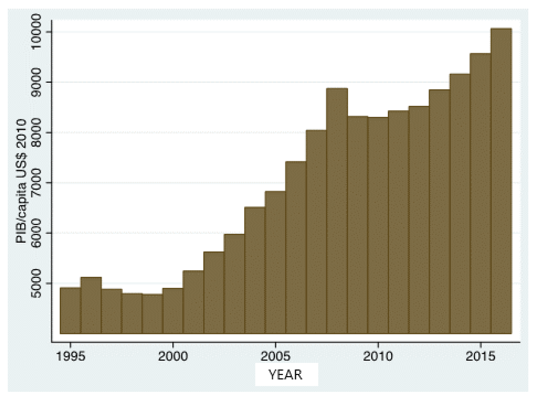
GDP per capita in Romania (1995–2016) in US dollars at constant prices in 2010. The source from which the data were taken was the World Bank website. Subsequently, this time series was logged, resulting in the InPIB secondary time series. In order to use the time series in specifying the optimal ECG test model, this time series was raised to square, resulting in the InPIB2 time series. The evolution of GDP per capita in Romania between 1995 and 2016 is described in the following
Figure 1.
- (b)
The Romanian Forest area (1995–2016) in thousands of hectares—two sources were used for the identification of the data that could be used in the model: FAOSTAT (Statistics from the Food and Agricultural Organization) and the records of the National Institute of Statistics in Romania. Following the preliminary test, the time series provided by the FAO was chosen. Considering that both time series are approximations of the realities regarding the forested area existing in Romania. The reason for choosing data from the FAO was the trend component that the time series presents and which is graphically identifiable. The trend in this time series will be helpful in testing the co-integration of the time series. At this stage of secondary processing, the growth rate of this variable was built. The total forest area remains constant in the period 2016–2020, as reported by FAO [
24].
Specifying and Running the Econometric Model
Following the study of specialty literature, presented in advance, two econometric ways for Kuznets’ environmental curve testing were highlighted either by panel (and panel model) or by time series, when the analysis targeted a single country. To verify the ECG hypothesis in Romania, we decided to use an econometric analysis method that is dedicated to time series—an ECVM (error correction vector) model. ECVM models represent a variation from autoregressive-vector-type (VAR) models for co-integrating time series.
Starting from the econometric model proposed by Yurttagüler and Kutlu [
12] (Equation (6)), we decided to sum up the quadratic form for testing the EKC hypothesis in Romania:
In this equation, the variable E_t is expressed by the forest growth rate (called for_gr) in Romania, and lnPIB and [lnPIB]2 represents the natural logarithm of GDP per capita (in USD, constant prices of the year 2010) and the square of this variable, respectively.
The first step in the development of the model consisted of testing the stationarity of the variables in the first-order difference. It turned out that the first-order variables are stationary for a confidence interval of 90% (the value of the statistical statistic is equal to 0.1 for the difference of the first order of forest growth rate and for this reason, this interval was chosen, higher than 95% confidence interval proposed by Fischer).
In the second stage, we ran the test of the optimal number of lags in the construction of the ECVM model. The results of this test led to the conclusion that the most stable model is one with two lags. The selection criteria FPE, AIC, HQIC and SBIC (four out of five criteria, as can be seen from the
Table 2) provided this information.
The next step was to test the cointegration of the time series. The concept of cointegration has been introduced in quantitative analysis by Granger (1983) [
25] and Engle and Granger (1987) [
26] and represents a property of chronological series that does not necessarily express a correlation between these series, but a linear combination of them is average and constant variance. Intuitively, it meaans that these time series are in a long-term equilibrium relationship. A Johansen test was run to test the cointegration with the mathematical form presented in Equation (10).
In this test, X_t represents a vector of variables, Δ= (1 − L) is the order difference 1, μ is a constant vector, where Π is the coefficient of the matrix with a low rank
r <
k, and
u_t is an innovation vector (Johansen, 1992) [
27]. The test also had the
r trend option, which was discussed in the data description section. This option includes a narrow trend in the model. The results of the Johansen co-integration test are shown in
Table 3. From these estimates, it results that there is a cointegration of the order 1, I (1), at the time series.
Based on the tests presented in the two tables, it was decided to use an ECVM model with two lags and with one cointegration equation. The results of the short-term model are presented in
Table 4.
From the above estimates, it results that the environment Kuznets curve hypothesis, using the evolution of the forest area in Romania as a variable for the state of the environment, is not supported. We observe the very high z-statistic values and also the very low value of R2 (this value is around 10 percent). However, the co-integration coefficient value is negative (_ce1L1 = −0.155), which denotes that the model and, implicitly, the relationship between the studied variables tends towards long-term equilibrium.
According to the cointegration equation in the table and the z-statistical indicators, it can be stated that the model is a statistically valid one in the long run. Therefore, the cointegration equation is the following:
Thus, the cointegration equation will have the following final form:
Next, the stability and autocorrelation tests of the specified model were run to see if the model was correctly specified and optimally calibrated. The error autocorrelation test (Lagrange multiplier) was run until the fourth lag, and the zero hypothesis that there is no autocorrelation error for a 95% confidence interval can be rejected. Thus, there is no indication of the model’s erroneous specification.
Estimates are presented in
Table 5.
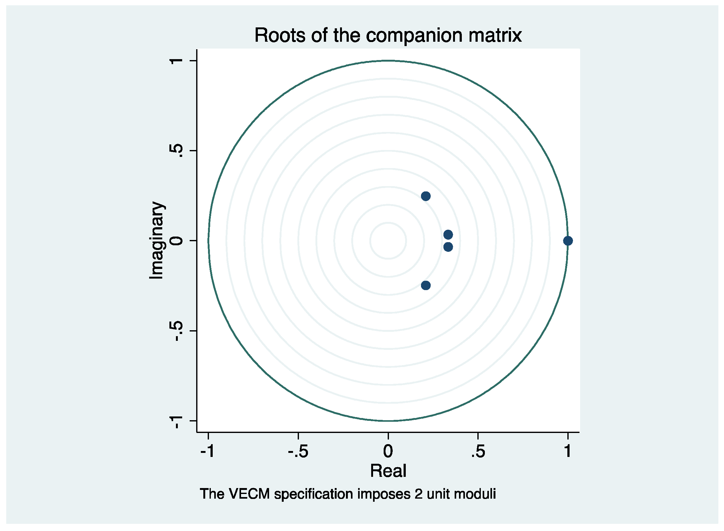
The next step involved testing the stability of the built model. For the CA that the specified pattern is stable, two eigen values equal to 1, and the rest of the subunit values, are required. This is apparent from the eigen value table (
Table 6). In the
Figure 2, two of the values must fit on the edge of the circle.
5. Conclusions
The environment and especially the forest resource are rather essential resources for life and for our future evolution as a society.
Based on the available data, the authors observed a decoupling process between the GDP growth that will not lead to a decrease in wooded areas in our country, thus verifying the Kuznets assumption of Romania’s environment curve.
As a result of the post-estimation tests, it emerged that the model is not statistically satisfactory in the short term, but it leads to long-term viable results. It was also found after the tests that the model was correctly specified and stable.
Compared to other Balkan countries, such as the western part of Turkey, Romania’s economic growth had a neutral to positive impact on the environment and especially on its forest area. Among the factors that confirm the Kuznets model are the migration of rural population towers urban centers (thus diminishing the demand for firewood), converting to natural gas as heating source and the decrease in intensive state-managed agriculture, which allowed the forest to slowly expand in the abandoned agricultural lands.
Sustainable development requires reaching an equilibrium between economic, social and environmental factors through soundly based policies and through impact studies, projects and community-based actions. Mainstreaming sustainability has to overcome various challenges, including the ones of assessing and measuring decoupling processes between economic development, the consumption of resources or social inequalities. In order to make it happen for any country, it is vital to have in place innovative public policies and instruments to implement them accordingly.
Protecting natural capital is a key element in ensuring sustainable development.
In this regard, increasing public awareness, the use of biomass in a sustainable way, preserving biodiversity and increasing forest areas are important actions to be undertaken in Romania. Moreover, the Recovery and Resilience Plan for Romania has the role to of being a stimulus for the implementation of reforms and investments in forestry areas and to better include the circular economy in relation to resource efficiency, material reuse and reducing waste.
Sustainable development has to be an adaptative process to national specificities if we want to have an impact on the long run to protect environment. Each country is endowed with different types of resources that need to be protected.
In the last years, progress has been made in Romania in the case of forestry resources, and the best example in this direction is the application of the Radar of Forests. However, there is a long way ahead, and many actions are needed to have a robust legislative framework, including an action plan for forestry resources or a dedicated bioeconomy or circular economy strategy that could better contribute to the protection of this precious resource.
The decoupling of the economic development from resource consumption in Romania is a process that builds on current and future initiatives. The model emphasized the trend towards long-term equilibrium when it comes to forestry resources.


 ,
, 


