Evolution Characteristics, Eco-Environmental Response and Influencing Factors of Production-Living-Ecological Space in the Qinghai–Tibet Plateau

Abstract

The Qinghai–Tibet Plateau (QTP) is a major “river source” and “ecological source” in China, as well as South Asia and Southeast Asia, and is a typical plateau region. Studying the evolution characteristics and ecological effects of the production-living-ecological space (PLES) of the QTP is of great practical significance and theoretical value for strengthening its ecological construction and environmental protection. Based on 30 m × 30 m land use/cover data of the QTP at five time-points of 1980, 1990, 2000, 2010, and 2020, this paper investigates the PLES evolution characteristics, transfer characteristics, eco-environmental response, and influencing factors of the eco-environmental quality index (EEQI) in the region of China of the QTP from 1980 to 2020 by land use transfer matrix, eco-environmental response model, hot spot analysis, and geographically weighted regression (GWR). The results show that: (1) from 1980 to 2020, the ecological space of the QTP decreased, while the production and living space saw an increase. The PLES pattern of the QTP showed a clear shift from 2000 to 2010, while there was no significant change from 1980 to 2000 and from 2010 to 2020. (2) From 1980 to 2020, the EEQI of the QTP decreased from 0.5634 in 1980 to 0.5038 in 2010, and then increased to 0.5044 in 2020, showing a changing trend of first decreasing and then increasing; the degradation of grassland ecological space to other ecological space was the main cause leading to ecological environment deterioration. (3) From 1980 to 2000, the EEQI was high in the midwestern and southeastern parts of the QTP, presenting a double-center distribution. From 2010 to 2020, the EEQI decreased in the western part, while the high value area in the eastern part increased significantly, obviously low in the west and high in the east. The spatial variation characteristics of hot and cold spots and EEQI are generally similar. (4) Natural ecological and socioeconomic factors have significant differences on the spatial distribution of EEQI in the QTP, and natural ecological factors are the main driving factors, with topographic relief having the strongest effect on EEQI as a natural ecological factor, and population density having the strongest effect as a socioeconomic factor.

1. Introduction

1.1. Background

Production-living-ecological space (PLES) is a combination of “production space, living space and ecological space”, which is the latest contribution of Chinese scholars to land use science [1]. Production space is the specific functional space where people engage in production activities, including agricultural and industrial production space; living space is the space used by people for daily activities, including rural and urban living space; ecological space is the natural environmental space, including forests, grasslands, waters and other ecological land. Production space provides material security for ecological and living space, living space is the necessary place for human economic activities to occur, and ecological space is the basis of PLES, supporting production and living space [2]. PLES may undergo conversion, and the occupation of ecological space by production space and living space is generally regarded as one of the major reasons for ecological environment degradation [3]. With the growth of the global population and economy, the rapid expansion of production space and living space in urban and rural areas [4] has led to a gradual reduction of ecological space and structural changes, which in turn, has resulted in a decline in eco-environmental quality [5,6]. However, at the same time, PLES optimization is also considered as an important way to adjust land use structure, intensive use of national land resources, and improvement of eco-environmental quality [7], and it is for this reason that the study of PLES has gradually become a hot spot in the academic community.

Land use evolution has traditionally been the focus of academic research, with topics focusing on the spatio-temporal patterns of land use change [8,9], driving force and driving mechanism [10,11], land use simulation and sustainable use [12,13], and other domains. In recent years, the eco-environmental response of land use has gradually become a hot spot for research, and the PLES theory proposed by Chinese scholars provides a new theoretical perspective for the study of land use evolution and eco-environmental response. China is one of big examples for case study on land use, as it has experienced a dramatic change in the land use structure of regions during more than four decades of rapid urbanization and industrialization, along with a variety of environmental problems, such as extensive land use and waste and ecological deterioration [14,15]. Therefore, scholars have conducted tons of studies on land use evolution in China. Nevertheless, China is still a country worthy of academic attention for case study, due to the fact that on the one hand, China’s vast territory contains a variety of geographic units with different landforms, such as plateaus, basins, plains, and hills, and under the influence of rapid urbanization and industrialization, the characteristics of land use change in typical regions still need to be continuously focused on. On the other hand, the central government put forward the reform idea of land spatial planning in 2019, and proposed the guiding idea of “promoting the construction of ecological civilization and optimizing the spatial structure of land” [16], showing that PLES and ecological environment optimization will be a big issue to be solved in the field of land use in China in the long run, and it is urgent for the academic community to complete the relevant theory.

1.2. Literature Review

This paper reviews the literature in terms of research subjects, research methods, research scales and influencing factors. As for the research objects, land use is one of the large global issues facing mankind [17,18], and many scholars have explored land use change in depth in the fields of geography, ecology and planning [19,20], with focus on land use transition [17,21], ecological effects and formation mechanisms of land use/land cover change (LULCC) [22], track of land use change [23] and influencing factors [24] and the like. Some scholars have also, from different perspectives such as landscape expansion index [25], ecosystem service value [26], land function [27,28], normalized difference vegetation index [29], enhanced vegetation index [30], net primary productivity [31], and soil erosion model [32], investigated land use, changes in ecological environment, and landscape patterns of land use [33,34]. As PLES has gradually evolved into an important theoretical direction for exploring land use change, many studies have started to probe land use problems in different regions under the framework of PLES, such as around PLES structural change patterns [35], spatio-temporal evolution characteristics of PLES conflicts [36,37], spatial agglomeration of PLES [38], spatial differentiation characteristics of mixed PLES multifunctional land use [39], and spatio-temporal pattern evolution of rural PLES [40] to provide decision reference for PLES conflict mitigation, regional ecological security pattern construction, national land space optimization, and ecological environment improvement [41,42].

For research methods and scales, most of the existing studies have been based on remote sensing image and geographic information systems to explore the land use transition, ecological response and its driving factors [43,44]. For land use change and transition, the center of gravity migration model and land use transfer matrix [45,46] are mainly adopted to analyze the characteristics of land use structure evolution. For the ecological response, the landscape pattern index and ecological environment response model are mostly used to figure out the evolution characteristics of ecological environment quality [47,48]. Studies are mostly centered on provincial/state [49], county [50,51], metropolitan area [52], urban agglomeration [53,54], watershed [55], and economic zone [56,57,58] scales to reveal the land use change characteristics and ecological response.

For the influence factors, the spatial heterogeneity model geographically weighted regression (GWR) [59] and the spatial homogeneity model geographical detector [60,61] are mostly borrowed to explore the spatial characteristics of the driving factors. The available studies have revealed that the factors affecting land use and ecological changes mainly include natural ecological factors and socioeconomic factors [62]. Natural ecological factors include climate [63,64], topography, vegetation and soil [65]. Socio economic factors include direct factors such as deforestation [66] and land reclamation [67], and indirect factors such as economy, population [68], traffic [69], technological development [70], and policy regime [71].

In summary, the available studies have explored land use change, spatial evolution of PLES, eco-environmental response and their influencing factors, but they are still insufficient. First of all, further study is required for the research object. Most of the current related papers focus on rapidly urbanizing areas and regions with high economic development, while less focus is given to special geographical regions such as plateaus. For typical regions, due to the special natural economic environment, their PLES change trends are fairly idiosyncratic, requiring the research to be further advanced. Secondly, the research methodology needs to be expanded. Most of the available studies are based on a geographic detector and other spatial homogeneity models to analyze the influencing factors of PLES evolution, land-use change, and land-use efficiency, while few studies resort to spatial heterogeneity models such as GWR to analyze the influencing factors of eco-environmental quality index (EEQI). GWR is a powerful tool for exploring the spatial heterogeneity of influencing factors and can better reflect the spatial heterogeneity of influencing factors, so it is important to introduce it to deeply reveal the driving mechanism of EEQI changes. Thirdly, the research indexes should be further optimized. Most of the current literature mainly explores the spatial evolution of PLES and the driving mechanism of its eco-environmental response from the perspective of natural elements or single indicators, while the driving role of socioeconomic elements and multi-indicator systems is under-considered. Therefore, this paper attempts to further deepen the existing research results.

1.3. Aim and Question

This paper focuses on the land use of the Qinghai–Tibet Plateau (QTP) in China and classifies the land use types of the QTP based on the PLES theory and five periods of land use/land cover data in 1980, 1990, 2000, 2010, and 2020. On that basis, this paper focuses on analyzing the PLES evolution characteristics of the QTP in different periods and analyzing its land-use transition by leveraging land-use transfer matrix. It also calculates the eco-environmental quality of QTP land use by the EEQI model and applies GWR to analyze the spatial differentiation of EEQI influencing factors. The purpose of this paper is to explore the land use evolution pattern and the corresponding eco-environmental response characteristics in the plateau region, with a view to providing a theoretical basis for land use optimization and eco-environmental protection in the QTP region of China and plateau regions of other countries, and to offer a reference for the development of related policies.

Therefore, this paper focuses on the following questions: (1) what are the characteristics of the spatio-temporal evolution pattern of PLES in the QTP, based on the data analysis of land use/land cover data?; what are the characteristics of land use transition?; (2) what are the characteristics of the spatio-temporal changes in EEQI due to the evolution of PLES? What are the spatial heterogeneity characteristics of influencing factors in the GWR model?

2. Models and Methods

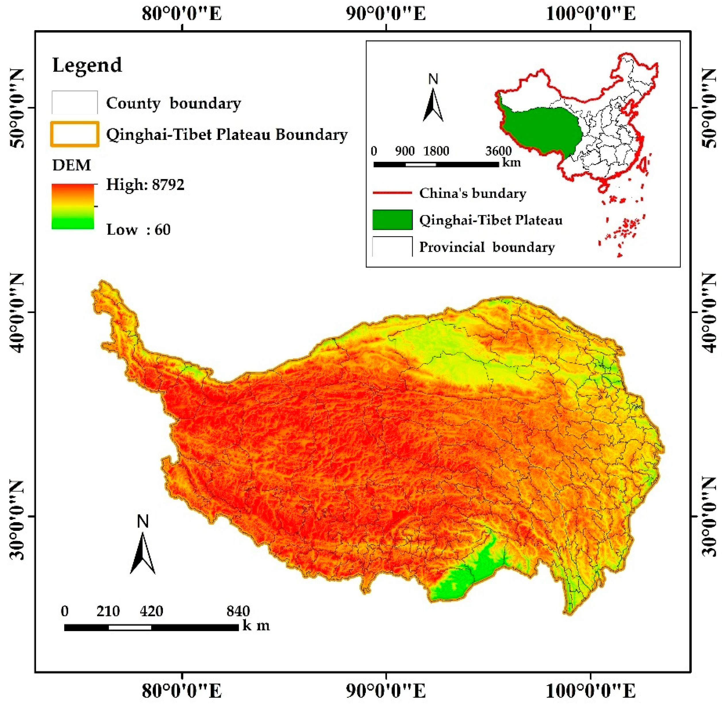
2.1. Research Area

The Qinghai–Tibet Plateau, known as “the Roof of the World”, is a typical plateau region, and is a “river source” and “ecological source” of China, as well as South Asia and Southeast Asia. Playing a role as the “initiator” and “regulator” of climate change in Asia and even the northern hemisphere, it is of great ecological importance. The QTP is distributed across nine countries; China, India, Pakistan, Tajikistan, Afghanistan, Nepal, Bhutan, Myanmar, and Kyrgyzstan. The study area in this paper is the part within China, ranging from 25°59′37″ N to 39°49′33″ N, 73°29′56″ E to 104°40′20″ E, covering an area of about 2542.30 × 103 km, with an average altitude of 4000 m above sea level, covering all or part of 6 provinces and regions of Tibet, Qinghai, Gansu, Sichuan, Yunnan and Xinjiang, involving a total of 216 county units (Figure 1). In 2019, there were more than 14 million permanent residents in the QTP, accounting for about 1% of the total across the country, with a resident population density of about 5.4 people/km², and the only cities with a population of over 1 million were Xining, Haidong, and Garze Tibetan Autonomous Prefecture. In 2019, the QTP had a GDP of over RMB 600 billion and a per capita GDP of about RMB 44,051, much lower than the national average of RMB 69,235, making it a typical sparsely populated area with lagging economic development.

This paper classifies PLES based on the classification criteria provided in the China Land Use/Land Cover Remote Sensing Monitoring Data Classification System [72]. Firstly, production space, living space, and ecological space are classified into two levels according to the functional attributes of PLES, and grassland, woodland, water and other ecological space are classified as ecological space, town and village living space are classified as living space, and industrial and agricultural production space are classified as production space. Secondly, the secondary types are divided into tertiary indicators according to the land use attributes, and a junction table between PLES structure and land use types is constructed (

Table 1. Classification of PLES function based on dominant function.

First Types	Secondary Types	Tertiary Indicators	Code
Production space	Agricultural production space	Paddy field, dry land	1
	Industrial production space	Industrial and mining traffic land	2
Living space	Urban living space	Urban land	3
	Rural living space	Rural residential land	4
Ecological space	Woodland ecological space	Woodland, shrubby woodland, sparse woodland, other woodlands	5
	Grassland ecological space	High coverage grassland, medium coverage grassland, Low coverage grassland	6
	Water ecological space	Canals, lakes, reservoirs and ponds, permanent glaciers and snow, beach land	7
	Other ecological space	Sandy land, gobi, saline alkali land, swamp land, bare land, bare rock land, other unused land	8

).

2.2. Research Methods

2.2.1. Land Use Transfer Matrix

The land use transfer matrix reflects both the quantitative changes of PLES land use and the transfer direction of PLES land use. In this paper, we get the land-use function transfer types and the land area for five time periods of 1980–1990, 1990–2000, 2000–2010, 2010–2020, 1980–2020 based on the superposition analysis of the land use data of the QTP by arcgis 10.2, and construction of a land-use function transfer matrix. It is calculated by the following equation:

$$S_{ij}=\left|\begin{array}{ccc}{\mathrm{S}}_{11}‥& {\mathrm{S}}_{12}‥& {\mathrm{S}}_{1\mathrm{n}}\\ {\mathrm{S}}_{21}‥& {\mathrm{S}}_{22}‥& {\mathrm{S}}_{2\mathrm{n}}\\ {\mathrm{S}}_{\mathrm{n}1\dots }& {\mathrm{S}}_{\mathrm{n}2}‥& {\mathrm{S}}_{\mathrm{nn}}\end{array}\right|$$

(1)

where S represents the area of land type conversion, i and j represent land-use types, n represents the number of land-use types, when i ≠ j, S_ij represents the area of type i land converted to type j land. A larger S_ij indicates more area of type i land converted to type j land and vice versa. When i = j, S_ij represents that the land type has not undergone an area transition, i.e., no transition has occurred to that land type.

2.2.2. Eco-Environmental Response Model

(1) EEQI. The EEQI can reflect the eco-environmental quality of the QTP intuitively. According to the available studies, the R-value (R_i) is used to show the ecological quality status of tertiary indicators in this paper. Most scholars have conducted studies by referring to R_i determined by Li [56], while some have adjusted R_i based on the conclusions reached by Li according to the characteristics of land type, precipitation, and climate in the study area. For example, Han [48] and Cui [57] revised R_i upwards to 0.3–0.5 for paddy fields and dry land; Yuan [43], Lv [49], Cui [57], Deng [73] and Hu [74] et al. adjusted R_i to 0.5–0.8 for grassland; Yuan [43], Han [48], Yang [54] and Cui [57] et al. resized R_i to 0.45 for swamp land and to 0.02–0.05 for sandy land and gobi. In this paper, proper adjustments are made to R_i of the corresponding sites according to the characteristics of the QTP. Firstly, because of the prominent role of agricultural production on ecological and environmental security and socioeconomic development in the QTP [75], R_i is adjusted to 0.3 for dry land and 0.35 for paddy fields. Secondly, since most of the QTP areas are dominated by grassland, which plays an important role in maintaining ecological environment quality, R_i is raised to 0.8 for high coverage grassland, to 0.75 for medium coverage grassland, and to 0.7 for low coverage grassland. Thirdly, R_i is revised to 0.45 for swamp land and to 0.05 for sandy land and gobi, as detailed in

Table 2. R-value of tertiary indicators.

Tertiary Indicators	R-Value	Tertiary Indicators	R-Value
Paddy field	0.35	Canal	0.60
Dry land	0.30	Lake	0.55
Industrial and mining traffic land	0.15	Reservoirs and pond	0.55
Urban land	0.20	Permanent glaciers and snow	0.90
Rural residential land	0.20	Beach land	0.45
Woodland	0.95	Sandy land	0.05
Shrubby woodland	0.65	Gobi	0.05
Sparse woodland	0.60	Saline alkali land	0.05
Other woodland	0.40	Swamp land	0.45
High coverage grassland	0.80	Bare land	0.05
Medium coverage grassland	0.75	Bare rock land	0.05
Low coverage grassland	0.70	Other unused land	0.05

. This paper uses Arcgis10.2 to count the area of all land types in the 216 county units of the QTP, and quantifies the overall characteristics of eco-environmental quality of each county unit in the study area as the ratio of the sum of eco-environmental quality (S_ki × R_i) of land use types in each county unit to the total area of that county. It is calculated by the following equation:

$${\mathrm{EEQI}}_{\mathrm{t}}=\sum _{\mathrm{i}=1}^{\mathrm{N}}\frac{{\mathrm{S}}_{\mathrm{ki}}}{{\mathrm{S}}_{\mathrm{k}}}{\mathrm{R}}_{\mathrm{i}}$$

(2)

where EEQI_t represents the EEQI at time node t; N represents the number of land-use types; S_ki represents the area of the land type i of the county unit at time t (km²); S_k represents the total area of the county (km²); R_i is the R-value of the land type i; N is the number of land types in the county. A larger EEQI_t indicates a higher eco-environmental quality of the corresponding area and vice versa.

(2) Ecological Contribution Rate. The ecological contribution rate refers to the degree of influence of land use function transformation on the change of regional eco-environmental quality. The contribution of different land types to eco-environmental quality has both positive and negative values. The analysis of both positive and negative sides helps to synthesize the type of land use that affects the change of eco-environmental quality and facilities distinguishing the dominant factors of ecological improvement and degradation of the QTP. It is calculated by the following equation:

$$\mathrm{ER}=\frac{\left({\mathrm{E}}_1-{\mathrm{E}}_0\right)\times {\mathrm{S}}_{\mathrm{i}}}{\mathrm{S}}$$

(3)

where ER represents the ecological contribution of land-use change type, E₁ and E₀ represent the EEQI at the end and the beginning of land type change, respectively; S_i represents the area of this land type changed (km²); S represents the total area of the study area (km²). A positive value of ER indicates that the eco-environmental quality of the QTP improves due to the change in this land-use type, while a negative value of ER indicates that the eco-environmental quality of the QTP decreases due to the change in this land-use type.

2.2.3. Hot Spot Analysis

Hot spot analysis, also known as the Getis–Ord ${\mathrm{G}}_{\mathrm{i}}^{*}$ tool, is widely used for socioeconomic and ecological analysis, where hot and cold spots represent the degree of aggregation in high and low-value spaces, respectively [76]. For an in-depth study of the spatial evolution characteristics of the eco-environmental quality in the QTP, this paper analyzes the spatial distribution of hot and cold spots of EEQI changes in the QTP based on the Getis–Ord ${\mathrm{G}}_{\mathrm{i}}^{*}$ tool in arcgis10.2, and then analyzes the spatial evolution characteristics of areas with better and worse eco-environmental quality in the QTP.

$${\mathrm{G}}_{\mathrm{i}}^{*}=\frac{{\sum }_{\mathrm{j}=1}^{\mathrm{n}}{\mathrm{w}}_{\mathrm{i},\mathrm{j}}{\mathrm{x}}_{\mathrm{j}}-\bar{\mathrm{x}}{\sum }_{\mathrm{j}=1}^{\mathrm{n}}{\mathrm{w}}_{\mathrm{i},\mathrm{j}}}{\mathrm{s}\sqrt{\frac{\mathrm{n}{\sum }_{\mathrm{j}=1}^{\mathrm{n}}{\mathrm{w}}_{\mathrm{i},\mathrm{j}}^2-{\left({\sum }_{\mathrm{j}=1}^{\mathrm{n}}{\mathrm{w}}_{\mathrm{i},\mathrm{j}}\right)}^2}{\mathrm{n}-1}}},\bar{\mathrm{x}}=\frac{{\sum }_{\mathrm{j}=1}^{\mathrm{n}}{\mathrm{x}}_{\mathrm{j}}}{\mathrm{n}},\mathrm{s}=\sqrt{\frac{{\sum }_{\mathrm{j}=1}^{\mathrm{n}}{\mathrm{x}}_{\mathrm{j}}^2}{\mathrm{n}}-{\left(\bar{\mathrm{x}}\right)}^2}$$

(4)

${\mathrm{G}}_{\mathrm{i}}^{*}$ directly visualizes the clustering position of high-value or low-value elements in space. Significantly positive ${\mathrm{G}}_{\mathrm{i}}^{*}$, with a larger value indicates a more obvious aggregation of high values in areas with better ecological quality in the QTP, which are called hot spots. On the contrary, there is a more obvious aggregation of low values in areas with poorer ecological quality, which are called cold spots. In the equation, ${\mathrm{w}}_{\mathrm{i},\mathrm{j}}$ represents the spatial weight between regions i and j, ${\mathrm{x}}_{\mathrm{j}}$ is the value of EEQI, $\bar{\mathrm{x}}$ is the mean of EEQI, s is the standard deviation of EEQI, and as for i, j = 1, 2, 3,..., n, n is the number of county units.

2.2.4. Geographically Weighted Regression

It has been shown that changes in eco-environmental quality are influenced by both the natural environment and socioeconomics, and the influence of both on eco-environmental quality is characterized by some spatial heterogeneity [77,78,79]. Therefore, this paper introduces GWR to explore the spatial heterogeneity pattern of the factors influencing eco-environmental quality of the QTP. The equation is as follows:

$${\mathrm{Y}}_{\mathrm{i}}={\mathrm{\alpha }}_0\left({\mathrm{u}}_{\mathrm{i}},{\mathrm{v}}_{\mathrm{i}}\right)+\sum _{\mathrm{k}=1}^{\mathrm{m}}{\mathsf{\alpha }}_{\mathrm{k}}\left({\mathrm{u}}_{\mathrm{i}},{\mathrm{v}}_{\mathrm{i}}\right){\mathrm{X}}_{\mathrm{ik}}+{\mathsf{\beta }}_{\mathrm{i}}$$

(5)

where Y_i represents the EEQI of region i, α₀ (u_i, v_i) represents the intercept, X_ik represents the value of explanatory variable k in region i, (u_i, v_i) represents the spatial coordinates of region i, α_k (u_i, v_i) represents the regression coefficient of explanatory variable k in region i, m represents the total number of explanatory variables, k represents the explanatory variable ordinal number, and β_i random error. If α_k(u_i, v_i) > 0, the explanatory variable K is positively correlated with EEQI and vice versa.

2.3. Influencing Factors

PLES evolution is a major cause leading to eco-environmental quality changes [80], and this paper focuses on the factors influencing the eco-environmental quality of the QTP from both natural ecological and socioeconomic dimensions. For the natural environmental factors, the QTP is in the main complex and diverse topography, with large differences in temperature and precipitation among districts and counties. Its ecological distribution is mostly influenced by precipitation, temperature, and elevation, and average annual precipitation, average annual temperature, and height above sea level are used as evaluation indexes in this paper; furthermore, NPP reflects the productivity of vegetation and has a direct effect on eco-environmental quality. Topographic relief and slope affect human activities, and thus, change land-use patterns that indirectly affect eco-environmental quality. Therefore, average annual precipitation, average annual temperature, height above sea level, topographic relief, slope, and NPP are used as natural ecological factors in this paper.

For socioeconomic factors, socioeconomic activities mainly include human daily activities, economic production activities, and construction activities [81,82,83]. Construction activities directly change land-use patterns, while human activities and economic activities directly influence construction activities and then indirectly affect land use. Therefore, economic density, population density, and nighttime light image are used as the indicators to represent economic activities, human activities, and construction activities in this paper; among them, the data on economic density and population density comes from Resource and Environment Science and Data Center (http://www.resdc.cn, accessed on 29 September 2021), the multi-factor weight distribution method is used to distribute the population data, and GDP data with the administrative area as the basic statistical unit to the spatial grid, the spatialization of population and GDP can be realized. Economic density is a reflection of regional economic development, while population density mirrors population density. A higher economic and population density indicates a greater demand for production space and living space, and thus, has a greater impact on the landscape pattern of the surrounding area. There are two ways to calculate urban nighttime light: one is to reflect urban development vitality by representing regional nighttime lighting intensity with the sum of pixel values of all illuminated areas within the nighttime area; the other is to reflect urban spatial expansion trends, land development intensity and construction scale by the sum of all light image pixels within the nighttime area, without considering the lighting intensity [84,85]. This paper leverages the latter method to calculate the nighttime light image to show the difference in construction intensity within the QTP. Therefore, economic density, population density, and nighttime light image are set as socioeconomic factors in this paper.

This paper chooses to analyze the influencing factors of EEQI of the QTP in 2010 mainly for the following reasons: Firstly, national ecological protection policies have been put forward in succession since 2010, leading to stricter requirements for ecological protection in the QTP. As a turning point of the ecological protection policy for the QTP, the year 2010 is typical. Secondly, some data from other years are missing, making it impossible to meet the research needs. In processing influencing factors, this paper extracts and converts raster data of the 216 county units of the QTP by the partition statistics tool of arcgis 10.2, as the base data are rasterized.

2.4. Research Steps and Data Source

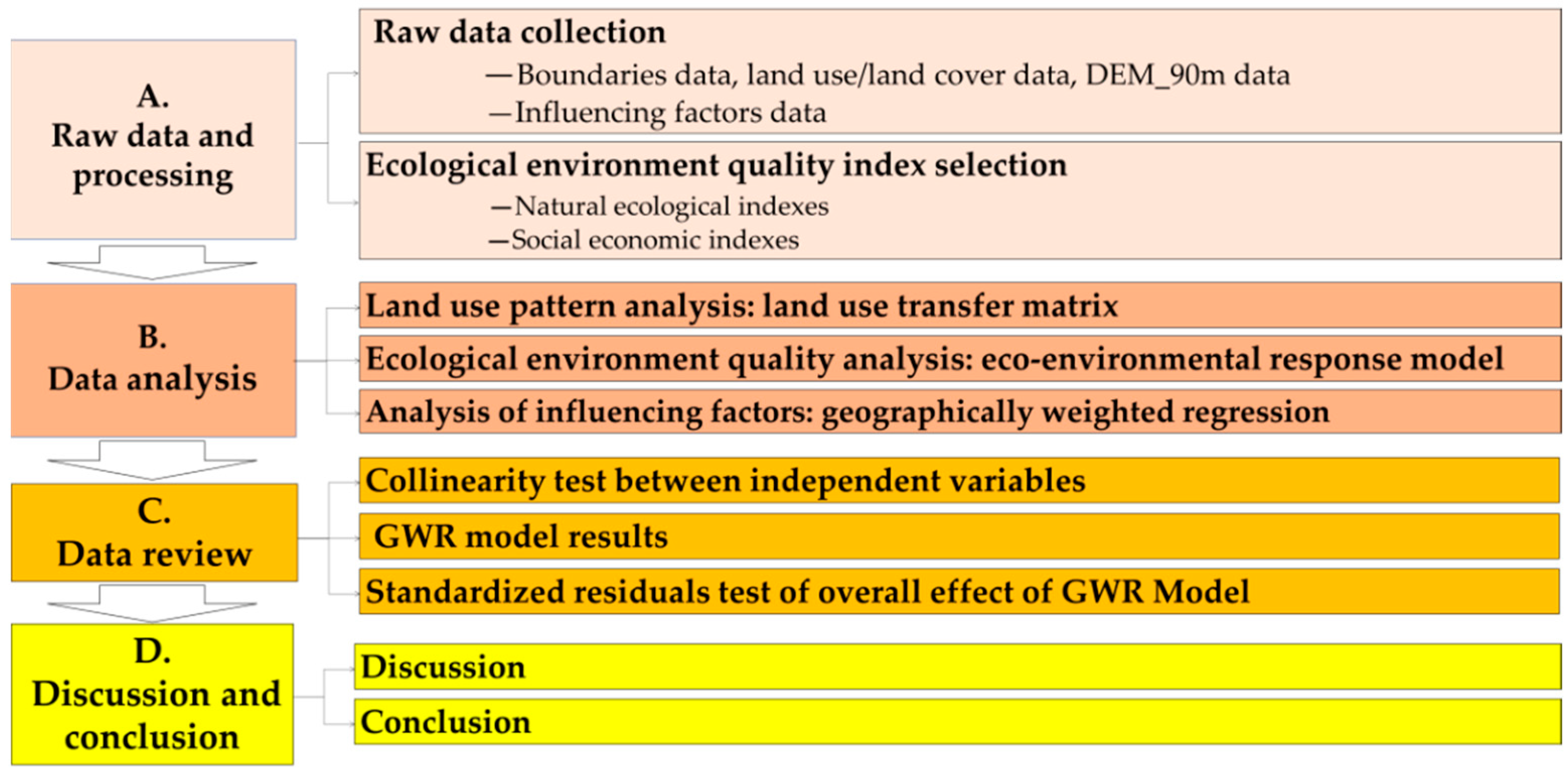
2.4.1. Research Steps

This paper mainly includes four steps. The first step is about raw data and processing, aiming to construct a junction table between PLES and land-use type, and to perform data computation and processing of land-use transfer matrix, ecological environment response model, and GWR based on arcgis10.2, python, and excel. The second step is data analysis, which is committed to analyzing the evolution characteristics of PLES, EEQI, and influencing factors of EEQI. The third step presents a data review to evaluate the GWR model for independent variable multicollinearity and operational parameters, and analyze the standardized residuals of the influencing factors as well as spatial differences. The fourth step is the Discussion and Conclusions (Figure 2).

2.4.2. Data Source

Among the data sources, the dependent variable EEQI was mainly obtained by calculating the remote sensing monitoring data of the land use, where the land use/land cover data include 30 m × 30 m raster data sets for 1980, 1990, 2000, 2010, and 2020. The independent variables include average annual precipitation, average annual temperature, height above sea level, topographic relief, slope, NPP, economic density, population density, and nighttime light image; the data were obtained from open source websites (

Table 3. Index selection and source.

Analysis Dimensions		Analysis Index	Data and Sources
Dependent variable		EEQI	Geographic Data Sharing Infrastructure, Resource and Environment Science and Data Center (http://www.resdc.cn, accessed on 29 September 2021)
Independent variable	Natural factors	Average annual precipitation	Geographic Data Sharing Infrastructure, Resource and Environment Science and Data Center (http://www.resdc.cn, accessed on 29 September 2021)
		Average annual temperature	Geographic Data Sharing Infrastructure, Resource and Environment Science and Data Center (http://www.resdc.cn, accessed on 29 September 2021)
		Topographic relief	Geographical Information Monitoring Cloud Platform (http://www.dsac.cn/, accessed on 29 September 2021)
		Height above sea level	Geospatial Data Cloud (http://www.gscloud.cn/search, accessed on 29 September 2021)
		Slope	Geospatial Data Cloud (http://www.gscloud.cn/search, accessed on 29 September 2021)
		NPP	National Qinghai–Tibet Plateau Science Data Center (http://data.tpdc.ac.cn/zh-hans/, accessed on 29 September 2021)
	Socioecono-mic factors	Economic density	Resource and Environment Science and Data Center (http://www.resdc.cn, accessed on 29 September 2021)
		Population density	Resource and Environment Science and Data Center (http://www.resdc.cn, accessed on 29 September 2021)
		Nighttime light image	Geographical Information Monitoring Cloud Platform (http://www.dsac.cn/, accessed on 29 September 2021)

). In addition, the DEM_90 m data used in this paper were obtained from the Geospatial Data Cloud (http://gscloud.cn, accessed on 29 September 2021), the vector boundaries data of the QTP were obtained from the National Qinghai–Tibet Plateau Science Data Center (http://data.tpdc.ac.cn/zh-hans/, accessed on 29 September 2021), and the county-level administrative boundaries data were obtained from the National Geomatics Center of China (NGCC) (http://www.ngcc.cn/ngcc/, accessed on 29 September 2021).

3. Results and Analysis

3.1. Spatio-Temporal Evolution Characteristic of PLES

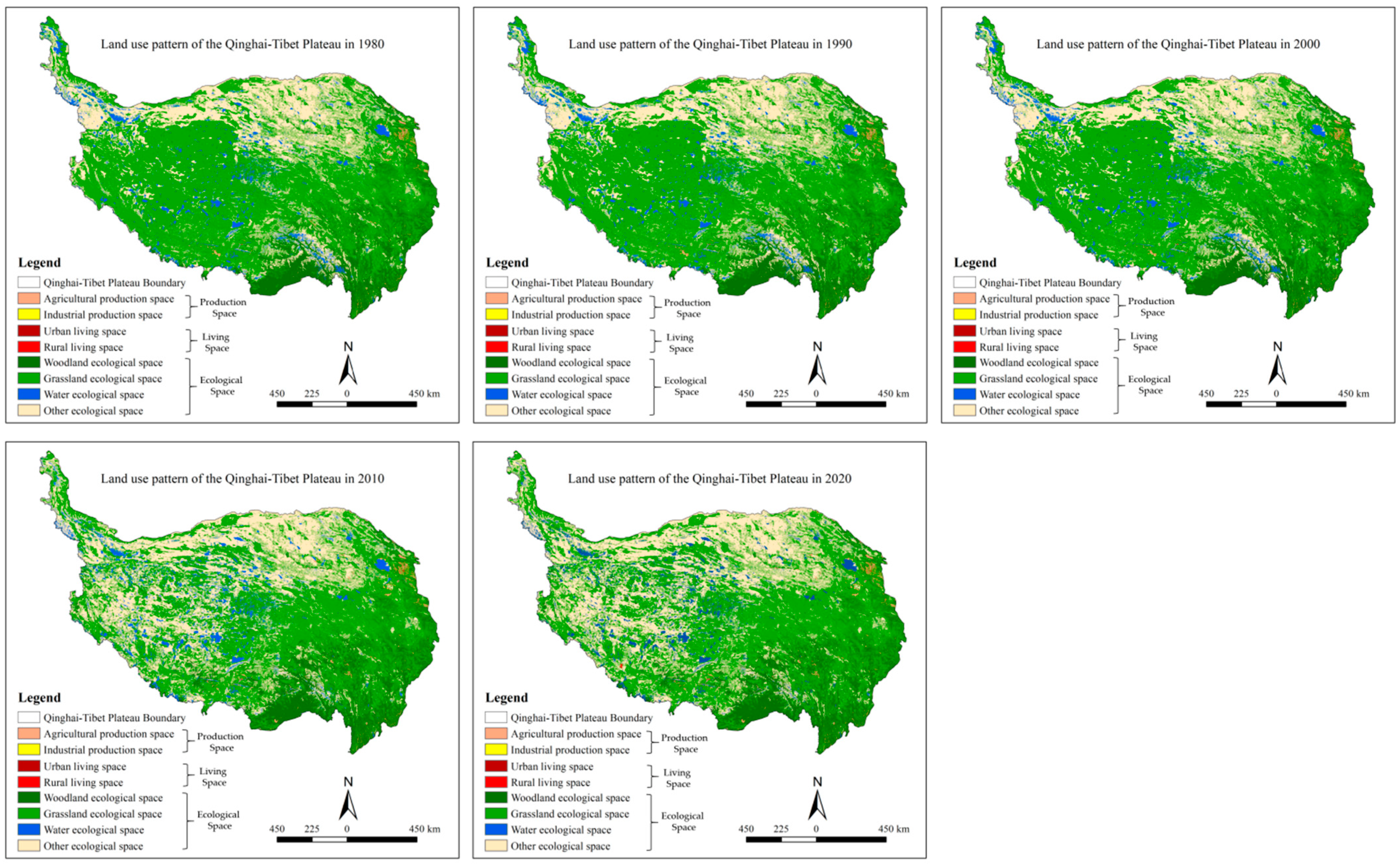
3.1.1. Spatial Evolution of PLES

In this paper, by reclassifying the land use/land cover data of the QTP from 1980 to 2020 by arcgis 10.2, we get the PLES distribution maps of the QTP for five time-points of 1980, 1990, 2000, 2010, and 2020 (Figure 3). In 1980, production space and living space accounted for a small proportion of the PLES of the QTP, and they were mainly located in the northeast and southwest, in a patchy distribution. The ecological space accounted for a large share, with ecological space of grassland and woodland mainly distributed in the west, east, and south, and other ecological space mainly in the north and northwest. The PLES in 1990 and 2000 showed similar distribution characteristics to those in 1980, presenting a general stabilization with insignificant changes. In 2010, production and living space in the PLES of the QTP increased obviously, while ecological space decreased. In particular, the grassland ecological space decreased sharply, while the land for other ecological spaces increased significantly, with the area changing mainly in the central and western regions of the QTP. The spatial distribution of PLES in 2020 was generally stable compared with that in 2010, with no significant changes.

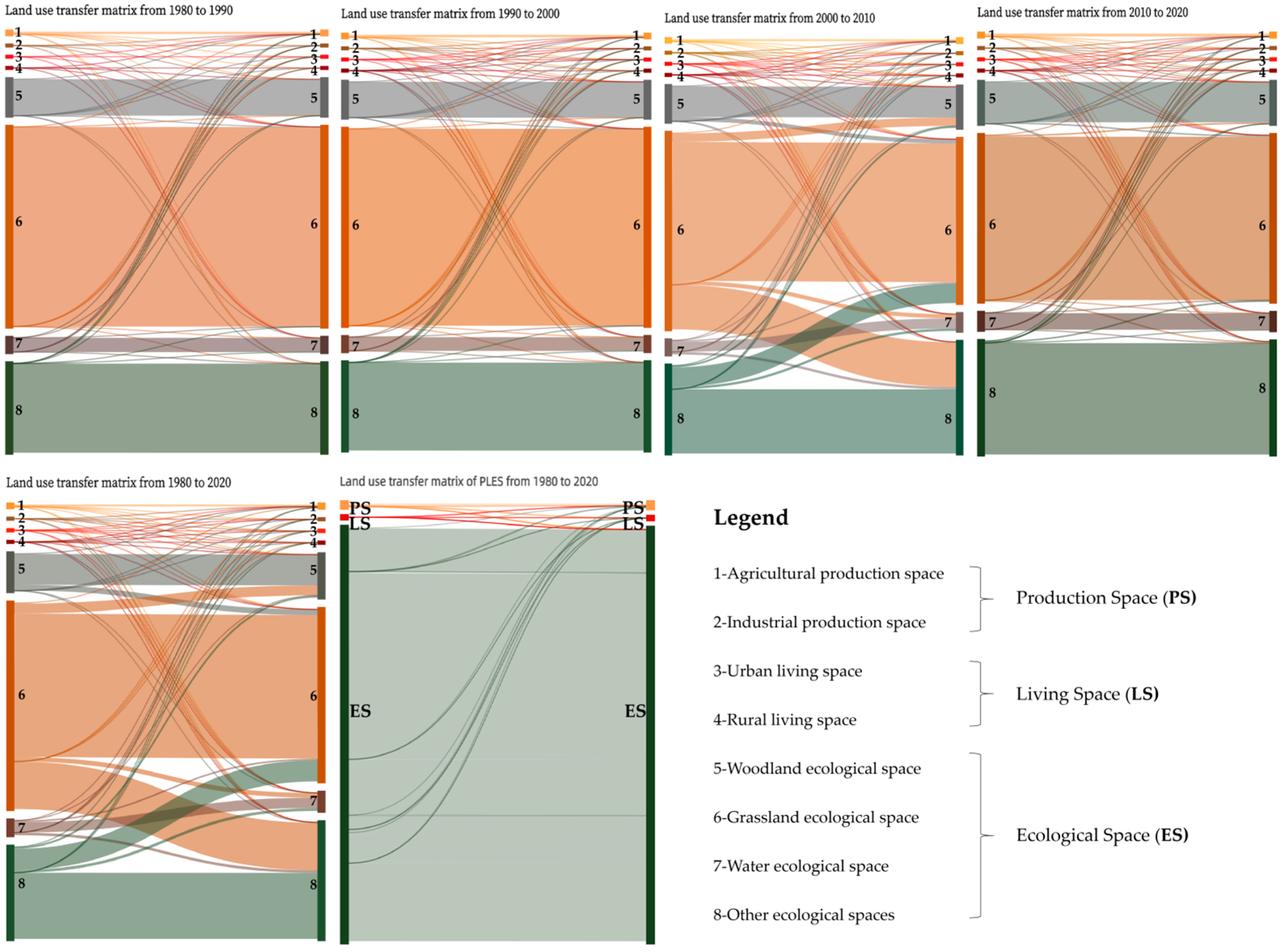
3.1.2. Land Use Transformation Characteristic of the PLES

By overlaying the land use/cover data of different years of the QTP based on Arcgis10.2, in this paper, we have obtained the land transfer area for the four time periods of 1980–1990, 1990–2000, 2000–2010, and 2010–2020, have constructed the land use transfer matrix (for details see attached

Table A1. Transfer matrix of land use structure change from 1980 to 1990 (km²).

Ecological Space (ES) Living Space (LS) Production Space (PS)		1990
		Grassland ES	Urban LS	Agricultural PS	Industrial PS	Woodland ES	Rural LS	Other ES	Water ES
1980	Grassland ES	15,203,540.21	95.41	2071.53	212.78	1083.68	12.16	3334.92	833.18
	Urban LS	10.31	1919.54	0.03	0	0	0	0	0.02
	Agricultural PS	62.18	58.61	191,183.55	26.7	44.03	5.83	25.03	576.19
	Industrial PS	27.26	0	0.03	2737.15	0.07	0	0.02	0
	Woodland ES	4390.1	0.04	13.54	0.01	2,766,179.84	0.05	257.27	3.29
	Rural LS	0.86	0	0.61	0	0.16	7670.8	0	0.05
	Other ES	2673.65	0.05	21.12	345.86	30.16	0	6,790,601.26	2676.85
	Water ES	500.13	0.03	101.84	83.47	170.87	0.06	3526.67	1,086,979.17

,

Table A2. Transfer matrix of land use structure change from 1990 to 2000 (km²).

Ecological Space (ES) Living Space (LS) Production Space (PS)		2000
		Grassland ES	Urban LS	Agricultural PS	Industrial PS	Woodland ES	Rural LS	Other ES	Water ES
1990	Grassland ES	1,518,415.3	19.9	493.18	7.65	251.94	9.17	978.74	944.56
	Urban LS	1.11	206.23	0.01	0	0.01	0	0	0
	Agricultural PS	17.86	17.89	19,239.54	0.53	4.93	22.46	13.36	22.64
	Industrial PS	0.06	0.04	0.01	340.44	0	0	0.04	0
	Woodland ES	704.3	1.54	41.81	0.03	275,972.66	0.35	19.22	10.91
	Rural LS	1.35	3.05	0.7	0	0.01	763.56	0.01	0.21
	Other ES	362.61	0.49	18.34	33.07	19.41	0.65	677,253.11	2086.54
	Water ES	777.66	0.07	11.7	2.19	63.23	0.14	2246.32	106,005.45

,

Table A3. Transfer matrix of land use structure change from 2000 to 2010 (km²).

Ecological Space (ES) Living Space (LS) Production Space (PS)		2010
		Grassland ES	Urban LS	Agricultural PS	Industrial PS	Woodland ES	Rural LS	Other ES	Water ES
2000	Grassland ES	1,074,815.29	86.14	5204.04	187.43	64,356.38	94.8	343,952.8	31,581.48
	Urban LS	3.81	230.45	8.2	1.37	1.96	0.52	1.78	1.13
	Agricultural PS	2147.09	63.24	15,921.66	15.21	1052.48	98.39	177.43	329.3
	Industrial PS	15.3	8.84	7.89	296.26	1.95	3.71	26.87	23.1
	Woodland ES	32,205.92	8.39	1575.72	8.5	238,053.79	10.23	3464.6	983.74
	Rural LS	26.27	6.56	46.21	1.09	4.67	703.47	2.94	5.12
	Other ES	150,559.89	4.16	238.37	324.7	14,185.57	3.07	496,670.83	18,523.32
	Water ES	10,117.58	8.25	154.23	33.37	1319.7	1.89	19,349.44	78,085.85

,

Table A4. Transfer matrix of land use structure change from 2010 to 2020 (km²).

Ecological Space (ES) Living Space (LS) Production Space (PS)		2020
		Grassland ES	Urban LS	Agricultural PS	Industrial PS	Woodland ES	Rural LS	Other ES	Water ES
2010	Grassland ES	1,244,348.56	52.64	847.58	152.68	11,257.04	85.8	10,095.2	2433.26
	Urban LS	14.97	356.62	28.19	0.63	3.06	7.66	2.57	2.35
	Agricultural PS	874.62	64.54	21,321.09	25.65	620.42	104.22	43.83	99.41
	Industrial PS	103.46	5.45	2.41	364.1	3.42	8.93	244.12	136.04
	Woodland ES	11,257.89	19.89	617.49	25.88	305,958.07	16.95	772.3	330.63
	Rural LS	50.24	7.51	86.98	1.07	10.49	752.86	4.16	2.59
	Other ES	11,226.32	305.62	50.39	119.63	850.41	17.81	847,461.94	3604.66
	Water ES	1788.41	9.4	91.95	5.89	240.09	2.48	1605.77	125,960.02

and

Table A5. Transfer matrix of land use structure change from 1980 to 2020 (km²).

Ecological Space (ES) Living Space (LS) Production Space (PS)		2020
		Grassland ES	Urban LS	Agricultural PS	Industrial PS	Woodland ES	Rural LS	Other ES	Water ES
1980	Grassland ES	1,057,141.96	447.99	6416.28	246.8	73,109.73	181.05	348,415.28	34,095.41
	Urban LS	5.68	163.58	15.15	0.15	1.07	4.93	0.59	1.84
	Agricultural PS	2702.41	134.54	13973	36.83	1498.41	187.12	200.9	457.46
	Industrial PS	42.4	12.76	6.89	161.52	3	7.42	36.6	5.85
	Woodland ES	41,813.73	17.34	2023.49	31.46	22,7891.45	24.76	3696.19	1121.7
	Rural LS	57.35	13.47	105.63	1.82	10.74	566.33	5.59	6.18
	Other ES	155,844.39	20.83	286.78	205.25	14,563.5	21.4	487,164.32	20,914.48
	Water ES	11,617.83	11.15	213.93	11.72	1380.04	3.73	20,149.91	75,506.13

), and created a land use transfer matrix Sankey diagram (Figure 4). The PLES transitions in the QTP from 1980 to 1990 and from 1990 to 2000 showed essentially similar characteristics, dominated by a shift from ecological space to production space and living space. During the period, the QTP saw a slight increase in the living space and production space, while a slight decrease in the grassland area in ecological space by about 10,348.8 km², mainly transformed into other ecological space, agricultural production space, and water space. The PLES of the QTP from 2000 to 2010 showed the most significant transition characteristics, also with a shift from ecological space to production space and living space. For ecological space, the largest reduction was found in grassland ecological space, by about 445,463.07 km², mainly transformed into other ecological space, woodland ecological space, and water ecological spaces. The PLES of the QTP from 2010 to 2020 continued the same transition, still dominated by the shift from ecological space to production and living space, with a decrease in intensity. In the ecological space, grassland ecological space was reduced by 24,924.18 km², and the reduction was mainly transformed into woodland ecological space and other ecological spaces.

In general, the PLES transition from 1980 to 2020 in the QTP was dominated by the transformation of ecological space to production space and living space, and the area transformed from the PLES in the QTP from 2000 to 2010 was higher than that from 1980 to 1990, from 1990 to 2000 and from 2010 to 2020. The area of island ecological space in the second land type of the PLES decreased, while the area of the other seven types of space was increased in the order of: other ecological space > woodland ecological space > water ecological space > agricultural production space > urban living space > industrial production space > rural living space. As for the reasons, first of all, high coverage of alpine grassland in the QTP and the changes in the growth environment of alpine vegetation in the Midwest with global warming are the main factors leading to grassland degradation. In addition, overgrazing and urbanization are also key factors leading to grassland degradation. Second, global warming has led to the ablation of a large amount of glacial snow in the QTP, as evidenced by the area decrease of glacial snow from 51,888.59 km² in 1980 to 39,708.59 km² in 2020, and the snow ablation is a significant cause for the increase of water space. Thirdly, the increased area of production space and living space in the QTP account for a small share of about 2% of the total, mainly because the QTP is a highland area not suitable for large human settlement and the scattered distribution of urban and rural areas leads to insignificant changes in the area of living and production space.

3.2. Eco-Environmental Response

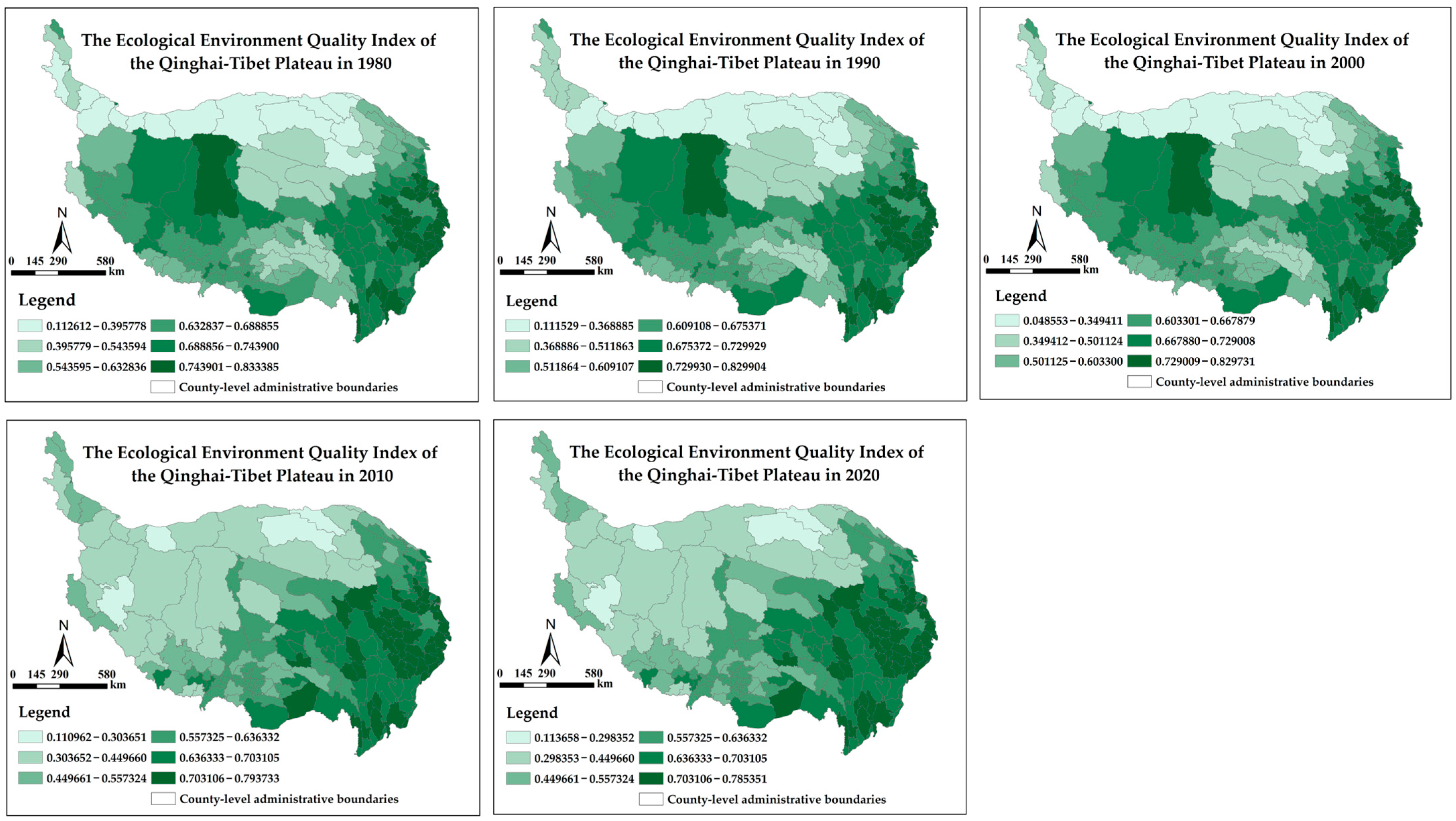
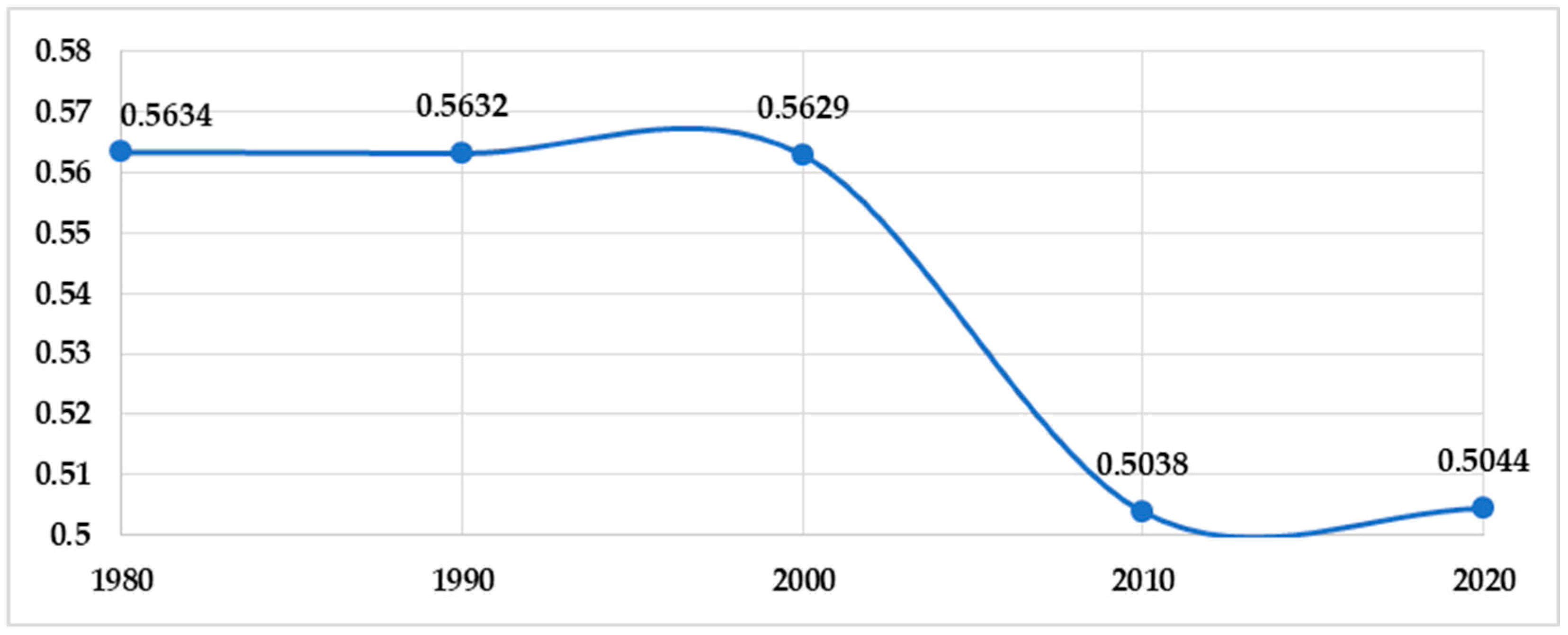
3.2.1. Change in Eco-Environmental Quality

The EEQI is used to measure regional eco-environmental quality, reflecting the changes in eco-environmental quality in the region, which may improve or deteriorate [56,57,58,59]. From 1980 to 2020, the EEQI of the QTP decreased from 0.5634 in 1980 to 0.5038 in 2010 and then increased to 0.5044 in 2020, showing a trend of decrease and then increase (

Table 4. EEQI of the QTP from 1980 to 2020.

Year	1980	1990	2000	2010	2020
EEQI	0.5634	0.5632	0.5629	0.5038	0.5044

). During that period, the transformation of grassland ecological space to other ecological spaces was a major factor leading to QTP deterioration of eco-environment, accounting for 82.608% of the total contribution. The conversion of other ecological space to grassland, woodland, and water ecological space was a major factor resulting in eco-environmental improvement, accounting for 93.199% of the total contribution. Agricultural and industrial production space, as well as rural and urban living space, had little influence on the improvement or deterioration of eco-environmental quality, accounting for a small share of the total contribution (

Table 5. The major PLES land use transformation types influencing eco-environmental quality, their contribution rate, and ratio from 1980 to 2020.

Improvement of Eco-Environment			Deterioration of Eco-Environment
Structure Transformation of PLES	Contribution Rate	Contribution Percentage	Structure Transformation of PLES	Contribution Rate	Contribution Percentage
Grassland–Woodland	0.000926	1.803%	Grassland–Agricultural production space	−0.00109	0.995%
Agricultural production Space–Grassland	0.000448	0.873%	Grassland–Other ecological space	−0.09081	82.608%
Agricultural production space–Woodland	0.000274	0.534%	Grassland–Water ecological space	−0.00288	2.619%
Other ecological space–Grassland	0.040142	78.167%	Woodland–Grassland	−0.0013	1.183%
Other ecological space–Water ecological space	0.003717	7.238%	Woodland–Agricultural production space	−0.0004	0.362%
Other ecological space–Woodland	0.004003	7.794%	Woodland–Other ecological space	−0.00106	0.965%
Water ecological space–Grassland	0.000874	1.702%	Woodland–Water ecological space	−0.00012	0.113%
Water ecological space–Woodland	0.000128	0.249%	Water ecological space–Other ecological space	−0.00364	3.314%
Total	0.050513	98.361%	Total	−0.10132	92.160%

). In general, from 1980 to 2020, the contribution rates of eco-environmental improvement and deterioration of eco-environmental quality in the QTP regions were 0.05 and −0.1, respectively, with the deterioration of eco-environmental quality over the improvement. Therefore, the EEQI of the QTP showed a downward trend.

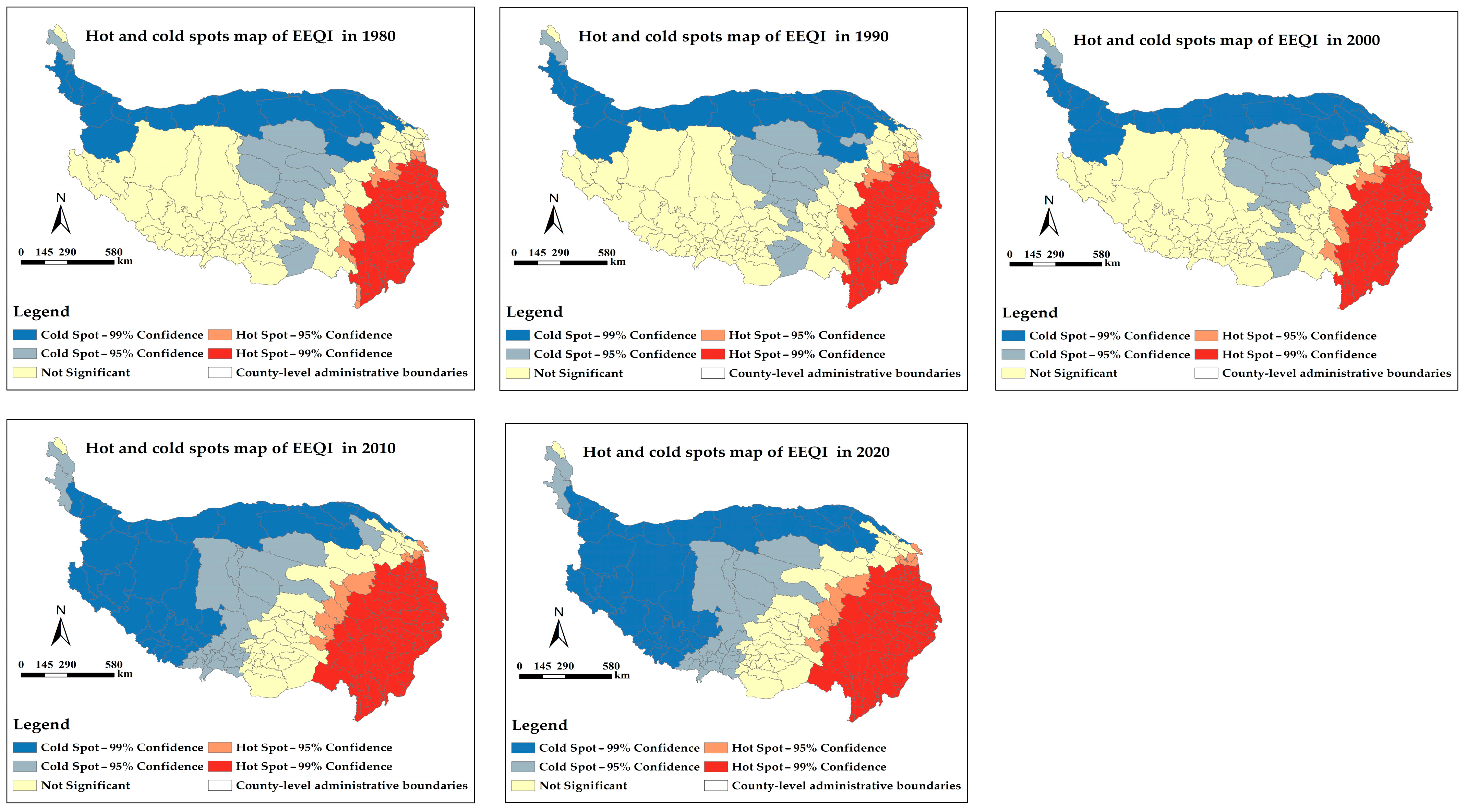
3.2.2. Spatial Characteristics of Eco-Environmental Quality

In this paper, the EEQI of 216 county-level administrative regions in the QTP was calculated and visually expressed through the arcgis 10.2 platform (Figure 5). The high EEQI area in the QTP in 1980 was mainly in the midwestern and southeastern regions, while the low-value area was mainly distributed in the northern, northwestern, and central parts, showing a bi-center spatial distribution. The distribution characteristics of the high and low EEQI areas in 1990 and 2000 were similar to those in 1980, and generally tended to be stable. In 2010, the spatial distribution of EEQI in the QTP changed greatly, with a slight increase in the north, a significant decrease in the high-value areas in the west, and a significant increase in the east, markedly “low in the west and high in the east”. The spatial distribution of EEQI in the QTP in 2020 had no significant change, except for an increased number of high-value areas, which were mainly distributed in the east and southeast. The distribution of high EEQI areas in the QTP from 1980 to 2020 changed from a bi-center in the midwest and southeast to a monocenter in the east, with a significant decline in eco-environmental quality in the west, with an improvement in eco-environmental quality in the east.

In this paper, we further analyzed the aggregation characteristics of EEQI in the QTP uaing the hot spot tool, with the use of Getis–Ord ${\mathrm{G}}_{\mathrm{i}}^{*}$ index in arcgis 10.2 (Figure 6). In 1980, the areas with a better ecological environment in the QTP were mainly distributed in the east and southeast, while the areas with a poorer ecological environment were mainly concentrated in the north, northwest, and middle. The distribution of cold and hot spots of the QTP eco-environmental quality changes in 1990 and 2000 showed essentially similar characteristics to those in 1980. The cold and hot spots of the QTP eco-environmental quality changes in 2010 and 2020 also showed similar distribution patterns, specifically, the areas with better ecological environment mainly distributed in the eastern and southeastern hot spots, with a significant increase, and the areas with poorer ecological environment mainly distributed in the northern, central, and western parts of the QTP.

Changes in ecological spatial patterns lead to changed EEQI, which, under the joint action of urbanization, industrialization, ecological restoration, and other socioeconomic factors, lead to the changes in the ecological and environmental patterns of the QTP, and then result in the evolution of EEQI. Due to the low level of economic development and lagged urbanization development in the QTP, they had little impact on the ecological environment and caused no significant changes in EEQI from 1980 to 2000. The rapid urbanization, with no effective protection of the ecological environment from 2000 to 2010, led to a decline in the ecological quality of the QTP and a large change in the spatial pattern of EEQI. The ecological environment quality of the QTP from 2010 to 2020 was improved compared to that from 2000 to 2010, mainly because that the Chinese government carried out ecological management by “Returning Cultivated Land into Forest and Grass” and ecological restoration, which to some extent counteracted the damage caused by human activities to the ecological environment, and thus pushed EEQI to grow slowly during that period. In addition, natural processes such as the melting of snow-capped mountains as a result of climate warming also have an impact on EEQI of the QTP.

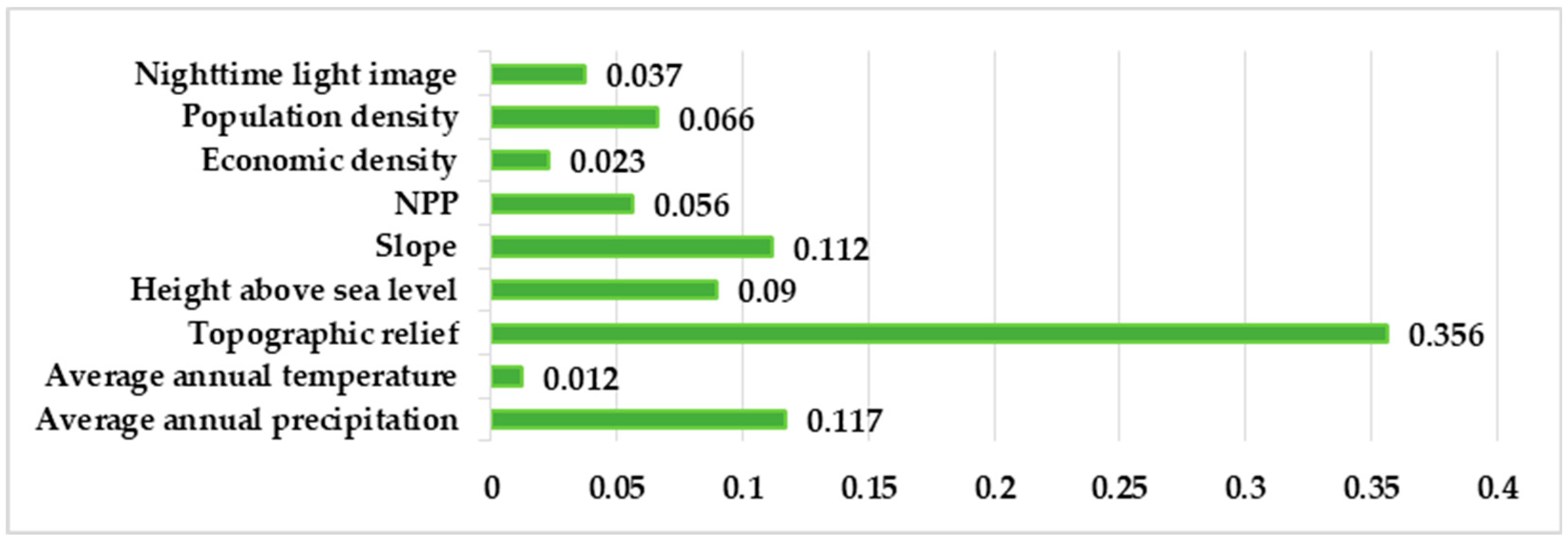
3.3. Influencing Factors Analysis

This paper analyzes the influencing factors of EEQI of the QTP using the GWR model and performs calculations in arcgis 10.2 with EEQI as a dependent variable, topographic relief, average annual precipitation, slope, height above sea level, population density, NPP, nighttime light image, economic density, average annual temperature as independent variables. Due to the large difference in magnitude of the absolute values of the nine influencing factors, they were first standardized to normalize all independent variables to the interval of (−1, 1), and then regression analysis was performed using the GWR model, and finally, the standardized residuals of the regression results of the 216 county units of the QTP and the regression coefficients of each independent variable were visually expressed (Figure 7). In the results, the standardized residuals were in the range of (−5.1, 4.7), with about 98.15% of the values in the range of (−2.5, 2.5), indicating the good performance of the model. According to the absolute values of correlation coefficients, the influencing factors by intensity are ranked as follows: topographic relief > average annual precipitation > slope > height above sea level > population density > NPP > nighttime light image > economic density > average annual temperature, as detailed below:

(1)

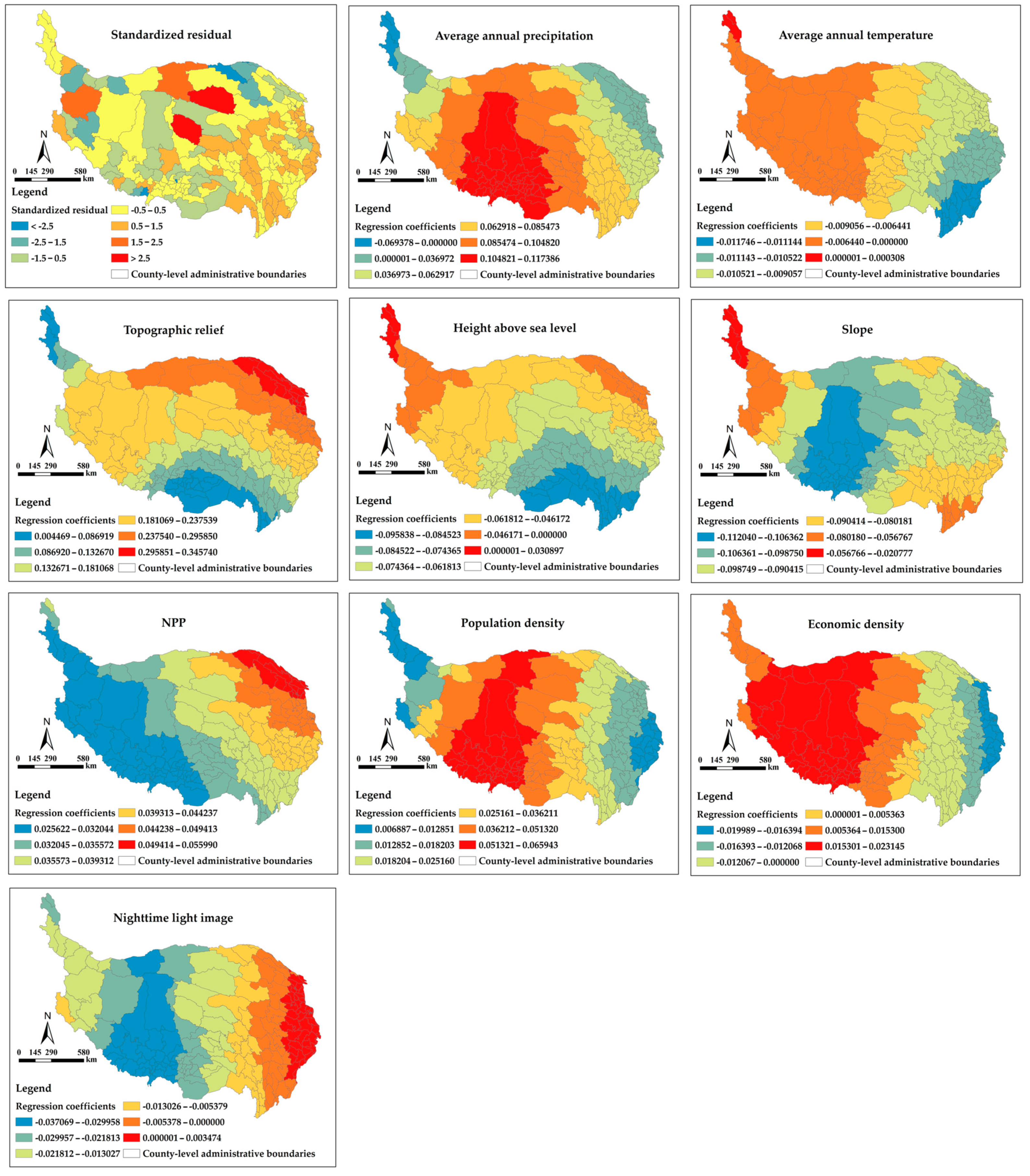
Average annual precipitation: The average annual precipitation of the QTP was predominantly positively correlated with EEQI, with the strength of the correlation decreasing gradually from the central part of the QTP to the east and west. A possible reason is that due to the complex natural environment and less average annual precipitation in the central part of the QTP, the vegetation in this region is sensitive to precipitation, resulting in a high correlation between the two and a greater contribution of precipitation to EEQI. In addition, due to plenty of water, the vegetation in the eastern and western parts of the QTP was less sensitive to precipitation than that in the central part, resulting in a lower contribution of average annual precipitation to EEQI [86].

(2)

Average annual temperature: The average annual temperature of the QTP was predominantly negatively correlated with EEQI, with the strength of the correlation decreasing from the southeast to the northwest of the QTP, reflecting that the limiting effect of temperature on EEQI was higher in the southeast than in the northwest. A primary reason is that there are significant differences in the adaptive capacity of vegetation to temperature in different areas. The significant height drop and temperature variation in the southeastern part of the QTP led to significant spatial stratification differences in vegetation, making the sensitivity of vegetation to temperature in this region more prominent, so the temperature had a greater limiting effect on EEQI in the southeastern part of the QTP [87]. The overall low temperature in the midwestern region and the distribution of hardy grassland vegetation in the region make the vegetation more adaptable to the temperature than in the southeast, so the limiting effect of average annual temperature on EEQI in the west-central region of the QTP was lower than that in the southeast.

(3)

Topographic relief: The topographic relief of the QTP was positively correlated with EEQI, with the correlation strength decreasing from northeast to northwest and south, showing a “stepped” spatial distribution. The large topographic relief in the south of the QTP tends to lead to landslides and soil erosion, and also exacerbates the difficulty of ecological protection, resulting in a smaller contribution of topographic relief to EEQI in the region. On the contrary, all the topographic relief in the northeastern part of the QTP was less undulating, thus, the vegetation growth conditions are better than those in the southern part, so the topographic relief contributed more to EEQI in the northeastern part of the QTP than in the southern part [88].

(4)

Height above sea level: The height above sea level of the QTP was mainly negatively correlated with EEQI, with the strength of the correlation decreasing in a circling pattern from south to northeast and northwest. The height above sea level was one of the major factors directly affecting vegetation species and distribution, with a large drop height in the south As the height above sea level rises, vegetation richness decreases, leaving the ecological environment more fragile, so the height above sea level had an enhanced limiting effect on EEQI in this region [89,90]. In contrast, the drop height in the northern region of the QTP was lower, and the vegetation types in this region were also homogeneous, resulting in a smaller limiting effect of elevation change on vegetation types and distribution, so the height above sea level had a lower limiting effect on EEQI in the north of the QTP [91].

(5)

Slope: The slope of the QTP was negatively correlated with EEQI, with the strength of the correlation decreasing from the central and eastern parts of the region to the southeast and northwest in descending order. The reasons for this were, first, that the central part of the QTP was mostly alpine grassland and other ecological lands with a fragile ecological environment and a larger slope led to a greater likelihood of erosion [92], and a stronger limiting effect on EEQI; second, the high level of urbanization in the eastern part of the QTP led to the encroachment of ecological space by construction activities in the region, making the limiting effect of slope on EEQI in the eastern part significantly higher [48,53].

(6)

NPP: NPP of the QTP was positively correlated with EEQI, with the strength of the correlation decreasing in a stepwise manner from the eastern to the western part, and the spatial heterogeneity was obvious. One of the main reasons is that NPP is a large indicator of EEQI, and the distribution of NPP was mainly influenced by vegetation richness and hydrothermal conditions. According to the above analysis, the vegetation growth environment in the western part of the QTP was inferior to that in the east and the vegetation richness in the west is much lower [87], resulting in a lower contribution of NPP to EEQI in the western part of the QTP than in the east.

(7)

Population density: The population density of the QTP is positively correlated with EEQI, with the strength of the correlation decreasing in steps from the central and western parts of the QTP to the eastern and western parts. A possible reason is that other ecological space (e.g., sandy land, gobi, swamp land et al.) in the central and western parts of the QTP has a higher share than in the eastern and western parts, and human activities transform other ecological land types with lower EEQI in the region into living and production land with higher EEQI; as a result, the contribution of population density to EEQI was higher in the western part of the QTP than in the eastern and western parts, which agrees with the findings of Li and Gao [56,58].

(8)

Economic density: Economic density in the west of the QTP was positively correlated with EEQI but negatively correlated in the east. First, the economy in the eastern part of the QTP was more developed than that in the central and western parts, and the economic activities caused certain damage to the ecological environment in the east, resulting in a prominent limiting effect on EEQI by the economic density in the eastern part. Second, other ecological spaces with lower EEQI accounted for a large proportion in the western part of the QTP, and economic activities transformed the other ecological land with a lower EEQI to land-use types with a higher EEQI (e.g., cultivated field, urban, and industrial land et al.), resulting in a prominent contribution of the western economic density to EEQI.

(9)

Nighttime light image: The nighttime light image of the QTP is predominantly negatively correlated with the EEQI, with a positive correlation in a small part of the eastern region and the strength of the correlation decreasing from the center to the east and west. The nighttime light image intuitively reflects the construction intensity and its expansion scale in the region. The above analysis shows that the ecological environment in the central part of the QTP is fragile, and construction activities tend to break its ecological environment, resulting in a high limiting effect of nighttime light image on EEQI there. The eastern part of the QTP is mainly composed of the Minshan Mountain Range and western Qinling Mountains with strong adaptability to the ecological environment, and the region is highly urbanized, increasing the intensity of ecological transformation in parallel with urban construction. Therefore, the nighttime light image of the area shows a certain contribution to EEQI.

4. Discussion

4.1. Change between Land Use and Land Cover

According to the above study, the ecological space of the QTP decreased, while production space and living space increased from 1980 to 2020, characterized by a degradation trend for the whole ecological environment. For the secondary land type, the land types of the QTP by change intensity from 1980 to 2020 are ranked as follows: grassland ecological space> other ecological space > woodland ecological space > water ecological space > agricultural production space > urban living space and industrial production space > rural living space (Figure 8), with the grassland ecological space decreasing in area, while the other seven types of space increasing. In the production and living space of the QTP, agricultural and industrial production space, urban living space increased by 0.05% of the total area, having a limited impact on the ecological quality of the QTP, and rural living space increased by 0.15%, reflecting that the main socioeconomic factor causing ecological degradation is the increase of rural settlements. In the ecological space of the QTP, the decrease in grassland ecological space accounted for 9.63% of the total, the increase in other ecological space accounted for 6.93% of the total area, and the increase in woodland and water ecological space accounted for 2.5% of the total area. The transformation of grassland ecological space into other ecological spaces is a major factor leading to the degradation of the ecological environment in the QTP. It differs from the land transformation in the more economically developed areas and in the plains. First, in the plains with rapid economic development, the changes in production and living space are greater than those in ecological space [43], and the transformation of the PLES is dominated by the shift of ecological space to production space [48], in particular, the land transformation in industrial economic zones is mainly showed as a continuous increase in production space, a continuous decrease in ecological space and a slight increase in living space [93]. Second, in areas dominated by ecological space (e.g., coastal zones), the production and living space is the land type with high variability [94]. It can be seen that the space transformation in the QTP was different from that in the plain areas, mainly because, firstly, the natural conditions of the QTP are complex and most of the areas are unsuitable for human life. Although production and living space increased, the increase was at a low percentage; secondly, the the QTP is vast and sparsely populated, and the ecological space was much larger in percentage than that of other regions, and human activities and economic development have limited impact on its space transformation. Therefore, the study of the QTP space transformation in this paper expands the research of land use evolution characteristics in plateau areas, which is helpful to explore and improve the relevant theories of land transition and ecological environment changes in plateau areas, and provides policy reference for space studies in plateau areas of other countries and regions.

4.2. Change Trend of EEQI

From 1980 to 2020, the EEQI changes of the QTP showed a general trend of decrease and then increase, with no significant changes from 1980 to 2000, but a sharp decrease in EEQI from 2000 to 2010, and a gradual improvement from 2010 to 2020 (Figure 9). An important reason is that the reform and opening-up from 1980 to 2000 promoted economic prosperity and led to the rapid development of urbanization. However, the QTP, located in northwest China, was underdeveloped in the economy, with lagging development of urbanization resulting in a small impact on the urbanization construction of the ecological environment and no obvious characteristics of EEQI changes. China started to implement the Strategy for Large-scale Development of Western from 2000 to 2010, and made every effort to promote the coordinated development of central and western China. During the period, the QTP development accelerated with the rapid advancement of the urbanization process. However, during the development, insufficient effective measures to protect the ecological environment led to a sharp decrease in grassland ecological space and a significant decline in EEQI. Since 2010, thanks to the national policy of “Returning Cultivated Land into Forest and Grass” and ecological restoration project, progress has been made in ecological governance. On the one hand, the state has strictly adhered to the concept of ecological protection in the process of land use and has taken remedial measures against illegal construction to ensure that the eco-environmental quality does not deteriorate throughout the development process; on the other hand, for areas where the ecology has been damaged due to regional development, ecological management has been carried out through “Returning Cultivated Land into Forest and Grass” and ecological restoration [95], so that the ecological environment in some areas has gradually improved, and the continuous deterioration of the eco-environmental quality of the QTP has been reversed.

4.3. Change of Influencing Factors in EEQI

This paper reveals that the EEQI influencing factors of the QTP by strength are in the order of topographic relief > average annual precipitation > slope > height above sea level > population density > NPP > nighttime light image > economic density > average annual temperature (Figure 10). Natural ecological factors are key driving factors influencing EEQI of the QTP, showing a distribution with obvious geographical and spatial differentiation. First, some findings of this paper are largely consistent with the conclusions of available papers. According to the studies, natural factors are an important basis for eco-environmental space in China and have a significant influence on eco-environmental quality [53]. Among the factors influencing the spatial differentiation of eco-environmental quality in rural areas of China, topographic factors are more influential, while social and economic factors are less influential [88]. In the Yellow River Delta region of China, natural conditions are the underlying factor influencing the spatial differentiation of eco-environmental quality, and the influence of socioeconomic factors on the spatial differentiation of eco-environmental quality is stable at a low level [48]. In southeastern Tibet, eco-environmental quality degradation is mainly the result of socioeconomic drivers, while changes in eco-environmental quality in other regions of Tibet are mainly influenced by natural factors such as temperature and precipitation [96]. Second, this study differs from other related studies as for the effect of population density on EEQI of the QTP, and finds that population density is positively correlated with EEQI, compared to the conclusion reached in the available studies that there is a negative correlation between population density and eco-environmental quality. The main reason is that the QTP land types differ from other areas in that there is a large proportion of other ecological lands with low EEQI, such as sandy land, gobi, swamp land, etc., and that human intervention may transform them into living and production space with high EEQI, such as cultivated field, urban and industrial land, resulting in the improvement of eco-environmental quality in this area, and a positive correlation between population density and EEQI. Compared with other regions, ecological space with small EEQI occupies a smaller portion, and human activities encroach on ecological space, leading to a negative correlation between population density and EEQI.

5. Conclusions

With the rapid development of the economy and society, the ecological space of different regions have been encroached and destroyed to a large extent, and the development coordination of the PLES has to be improved. In this context, how to promote the coordinated development of production, living and ecological spaces is a major theoretical issue that needs to be addressed urgently. This paper explores the evolution of the PLES pattern and changing characteristics of eco-environmental quality in the QTP from 1980 to 2020 based on the land-use transfer matrix, ecological environment response model, hot spot analysis, and analyzes the influencing factors of EEQI in 216 county units of the QTP using the GWR model. The main conclusions reached are presented as follows:

(1)

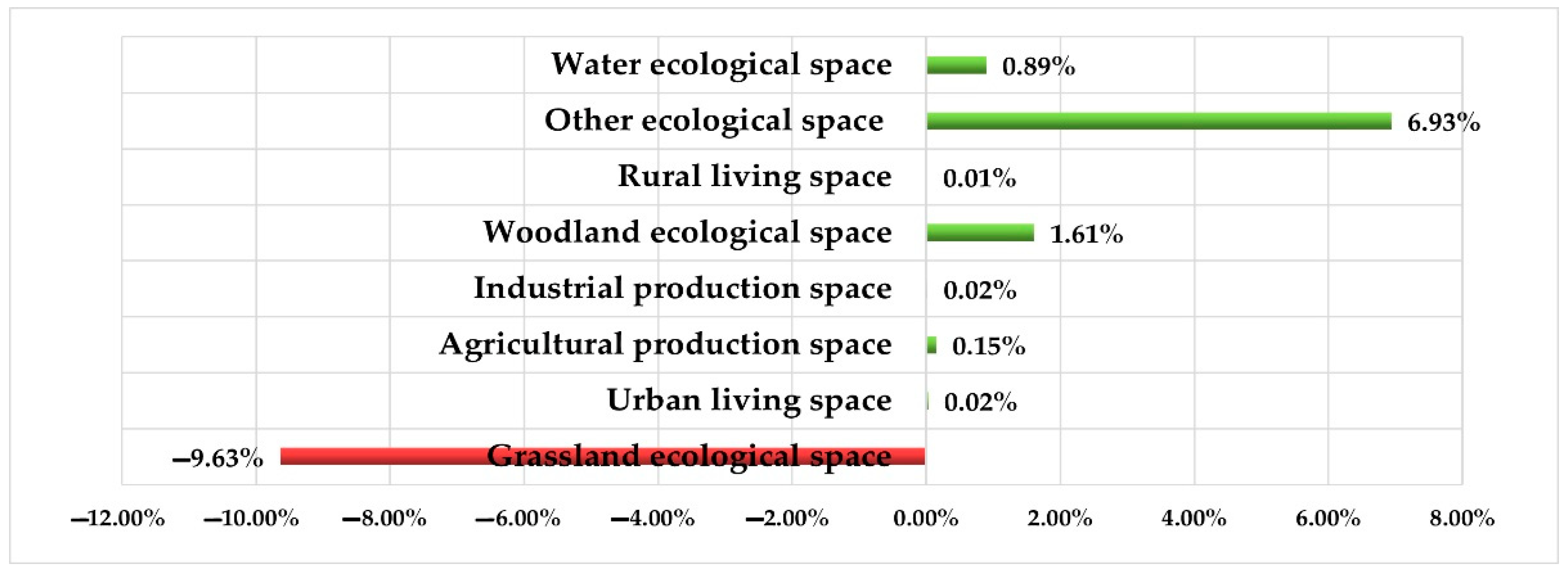
There are obvious change nodes in the spatial evolution of the PLES of the QTP, and the change of the PLES pattern shows obvious shift nodes from 2000 to 2010, and there were no significant changes in PLES evolution patterns in the two periods of 1980–2000 and 2010–2020. From 1980 to 2020, the ecological space in the QTP decreased and the production and living space increased. In terms of transition of the secondary land type, the PLES pattern of the QTP showed a decrease in the area of grassland ecological space and an increase in the area of woodland ecological space, water ecological space, other ecological space, agricultural production space, industrial production space, urban living space, and rural living space.

(2)

There was a large spatial heterogeneity in the spatial distribution of EEQI in the QTP, with higher EEQI in the midwestern and southeastern parts of the QTP from 1980 to 2000, and low-value areas mainly distributed in the central, northern, and northwestern parts of the QTP, in a bi-center spatial distribution. The hot spots of EEQI were mainly distributed in the east and southeast, while the cold spots were mainly concentrated in the north, northwest, and middle. The spatial changes of EEQI from 2010 to 2020 were obvious, characterized by the disappearance of the high-value area of EEQI in the central and western regions, the expansion of the low-value areas to the west, the gradual movement of the high-value areas to the southeast of the QTP, the obvious increase of the high-value areas in the east and southeast, prominent in the distribution characteristic of low west and high east. The hot spots of EEQI are mainly distributed in the eastern and southeastern hot spots, with a significant increase, while the cold spots are mainly distributed in the northern, central, and western parts of the QTP.

(3)

The effects of natural ecological and socioeconomic factors on the spatial distribution pattern of EEQI of the QTP differed significantly, which are, by strength, ranked as follows: topographic relief > average annual precipitation > slope > height above sea level > population density > NPP > nighttime light image > economic density > average annual temperature, with natural ecological factors being main driving factors. The strongest effect of topographic relief on EEQI was found among natural ecological factors, and the strongest effect of population density on EEQI was among socioeconomic factors.

This paper provides new ideas for the coordinated development of land use, ecological environment protection, and the PLES in plateau areas. Theoretically, it explores the evolutionary pattern of the PLES and the change characteristic of eco-environmental response in the plateau region, facilitating a deep understanding of the evolutionary pattern of space in the plateau region. Practically, the findings of this paper can help the government and policymakers to find a reasonable model for the protection of the plateau ecological environment. It is not only applicable to the plateau region of China but also provides a reference for space and ecological, environmental protection in the plateau region of other countries and regions. However, there are some limitations to this paper. First, this paper analyzes the change characteristic of the QTP eco-environmental quality only based on land use/land cover data but involves no specific changes in the QTP eco-environmental environment by field research, as a result, it cannot fully reflect the real situation of the QTP eco-environmental quality, and the conclusion needs further verification. Second, this paper selects the influencing factors based on the typical characteristics of the QTP, not covering all factors. Therefore, the degree of influence of other factors such as slope direction, NDVI, soil type, industrial structure, and infrastructure level on the ecological quality of the QTP needs to be further verified. The authors will continue to deepen the research on these two limitations in the subsequent study.

References

1. Fan, J.; Zhou, K.; Chen, D. Innovation and Practice of Economic Geography for Optimizing Spatial Development Pattern in Construction of Ecological Civilization. Econ. Geogr. 2013, 33, 1–8. [Google Scholar] [CrossRef]
2. Yang, Y.; Bao, W.; Li, Y.; Wang, Y.; Chen, Z. Land Use Transition and Its Eco-Environmental Effects in the Beijing–Tianjin–Hebei Urban Agglomeration: A Production–Living–Ecological Perspective. Land 2020, 9, 285. [Google Scholar] [CrossRef]
3. Fan, J. Draft of major function oriented zoning of China. Acta Geogr. Sin. 2015, 70, 186–201. [Google Scholar] [CrossRef]
4. Wang, S.H.; Huang, L.; Xu, X.L.; Li, J.H. Spatio-temporal variation characteristics of ecological space and its ecological carrying status in mega-urban agglomerations. Acta Geogr. Sin. 2022, 77, 164–181. [Google Scholar] [CrossRef]
5. Yu, Z.S.; Cheng, Y.Q.; Li, X.J.; Sun, D.Q. Spatial evolution process, motivation and restructuring of “production-living-ecology” in industrial town: A case study on QugouTown in Henan Province. Sci. Geogr. Sin. 2020, 40, 646–656. [Google Scholar] [CrossRef]
6. Ling, Z.Y.; Li, Y.S.; Jiang, W.G.; Liao, C.M.; Ling, Y.R. Dynamic Change Characteristics of “Production-living-ecological Spaces” of Urban Agglomeration Interlaced with Mountains, Rivers and Sea: A Case Study of the Beibu Gulf Urban Agglomeration in Guangxi. Econ. Geogr. 2022, 42, 18–24. [Google Scholar] [CrossRef]
7. Hu, W.T.; Wang, L.G.; Shu, M.H. Reflections on delimiting the three basic spaces in the compilation of Urban and Rural plans. City Plan. Rev. 2016, 40, 21–26. [Google Scholar] [CrossRef]
8. Dewan, A.M.; Yamaguchi, Y. Land use and land cover change in Greater Dhaka, Bangladesh: Using remote sensing to promote sustainable urbanization. Appl. Geogr. 2009, 29, 390–401. [Google Scholar] [CrossRef]
9. Lambin, E.F.; Geist, H.J.; Lepers, E. Dynamics of land-use and land-cover change in tropical regions. Annu. Rev. Environ. Resour. 2003, 28, 205–241. [Google Scholar] [CrossRef] [Green Version]
10. Lambin, E.F.; Turner, B.L.; Geist, H.; Agbola, S.B.; Angelsen, A.; Bruce, J.W.; Coomes, O.T.; Dirzo, R.; Fischer, G.; Folke, C.; et al. The causes of land-use and land-cover change: Moving beyond the myths. Glob. Environ. Chang. Hum. Policy Dimens. 2001, 11, 261–269. [Google Scholar] [CrossRef]
11. Verburg, P.H.; Schot, P.P.; Dijst, M.J.; Veldkamp, A. Land use change modelling: Current practice and research priorities. GeoJournal 2004, 61, 309–324. [Google Scholar] [CrossRef]
12. Tan, R.; Liu, Y.; Zhou, K.; Jiao, L.; Tang, W. A game-theory based agent-cellular model for use in urban growth simulation: A case study of the rapidly urbanizing Wuhan area of central China. Comput. Environ. Urban Syst. 2015, 49, 15–29. [Google Scholar] [CrossRef]
13. Kates, R.W.; Clark, W.C.; Corell, R.; Hall, J.M.; Jaeger, C.C.; Lowe, I.; Mccarthy, J.J.; Schellnhuber, H.J.; Bolin, B.; Dickson, N.M.; et al. Sustainability science. Science 2001, 292, 641–642. [Google Scholar] [CrossRef] [PubMed]
14. Liu, J.L.; Liu, Y.S.; Li, Y.R. Classification evaluation and spatial-temporal analysis of “production-living-ecological” spaces in China. Acta Geogr. Sin. 2017, 72, 1290–1304. [Google Scholar] [CrossRef]
15. Liu, P.F.; Sun, B.D. The spatial pattern of urban production-living-ecological space quality and its related factors in China. Geogr. Res. 2020, 39, 13–24. [Google Scholar] [CrossRef]
16. General Office of the State Council of the People’s Republic of China (GOSC). Several Opinions on Establishing a Land Spatial Planning System and Supervising Its Implementation; GOSC: Beijing, China, 2019. [Google Scholar]
17. Arrow, K.; Bolin, B.; Costanza, R.; Dasgupta, P.; Folke, C.; Holling, C.S.; Jansson, B.O.; Levin, S.; Maler, K.G.; Perrings, C.; et al. Economic growth, carrying capacity, and the environment. Science 1995, 268, 520–521. [Google Scholar] [CrossRef]
18. Liu, Y.; Huang, X.; Yang, H.; Zhong, T. Environmental effects of land-use/cover change caused by urbanization and policies in Southwest China Karst area: A case study of Guiyang. Habitat Int. 2014, 44, 339–348. [Google Scholar] [CrossRef]
19. Long, H.L. Land use transition and land management. Geogr. Res. 2015, 34, 1607–1618. [Google Scholar] [CrossRef]
20. Wu, J.S.; Feng, Z.; Gao, Y.; Peng, J. Research on ecological effects of urban land policy based on DLS model: A case study on Shenzhen City. Acta Geogr. Sin. 2014, 69, 1673–1682. [Google Scholar] [CrossRef]
21. Rind, D. Complexity and climate. Science 1999, 284, 105–107. [Google Scholar] [CrossRef] [Green Version]
22. Du, X.; Huang, Z. Ecological and environmental effects of land use change in rapid urbanization: The case of Hangzhou, China. Ecol. Indic. 2017, 81, 243–251. [Google Scholar] [CrossRef]
23. Skokanová, H.; Havlíček, M.; Borovec, R.; Demek, J.; Eremiášová, R.; Chrudina, Z.; Mackovčin, P.; Rysková, R.; Slavík, P.; Borovec, R.; et al. Development of land use and main land use change processes in the period 1836–2006: Case study in the Czech Republic. J. Maps 2012, 8, 88–96. [Google Scholar] [CrossRef] [Green Version]
24. Chang, Y.; Hou, K.; Li, X.; Zhang, Y.; Chen, P. Review of land use and land cover change research progress. In Conference Series: Earth and Environmental Science; IOP Publishing: Bristol, UK, 2018; Volume 113, p. 012087. [Google Scholar] [CrossRef]
25. Dadashpoor, H.; Azizi, P.; Moghadasi, M. Land use change, urbanization, and change in landscape pattern in a metropolitan area. Sci. Total Environ. 2019, 655, 707–719. [Google Scholar] [CrossRef] [PubMed]
26. Song, W.; Deng, X. Land-use/land-cover change and ecosystem service provision in China. Sci. Total Environ. 2017, 576, 705–719. [Google Scholar] [CrossRef]
27. O’Sullivan, L.; Wall, D.; Creamer, R.; Bampa, F.; Schulte, R.P.O. Functional Land Management: Bridging the Think-Do-Gap using a mult-stakeholder science policy interface. Ambio 2018, 47, 216–230. [Google Scholar] [CrossRef] [Green Version]
28. Wastfelt, A.; Zhang, Q. Keeping agriculture alive next to the city: The functions of the land tenure regime nearby Gothenburg, Sweden. Land Use Policy 2018, 78, 447–459. [Google Scholar] [CrossRef]
29. Li, Y.; Cao, Z.; Long, H.; Liu, Y.; Li, W. Dynamic analysis of ecological environment combined with land cover and NDVI changes and implications for sustainable urban- rural development: The case of Mu Us Sandy Land, China. J. Clean. Prod. 2017, 142, 697–715. [Google Scholar] [CrossRef]
30. Matsushita, B.; Yang, W.; Chen, J.; Onda, Y.; Qiu, G. Sensitivity of the Enhanced Vegetation Index (EVI) and Normalized Difference Vegetation Index (NDVI) to topographic effects: A case study in high-density cypress forest. Sensors 2007, 7, 2636–2651. [Google Scholar] [CrossRef] [Green Version]
31. Plutzar, C.; Kroisleitner, C.; Haberl, H.; Fetzel, T.; Bulgheroni, C.; Beringer, T.; Hostert, P.; Kastner, T.; Kuemmerle, T.; Lauk, C.; et al. Changes in the spatial patterns of human appropriation of net primary production (HANPP) in Europe 1990–2006. Reg. Environ. Chang. 2016, 16, 1225–1238. [Google Scholar] [CrossRef]
32. Borrelli, P.; Robinson, D.A.; Fleischer, L.R.; Lugato, E.; Ballabio, C.; Alewell, C.; Meusburger, K.; Modugno, S.; Schütt, B.; Ferro, V.; et al. An assessment of the global impact of 21st century land use change on soil erosion. Nat. Commun. 2017, 8, 2013. [Google Scholar] [CrossRef] [Green Version]
33. Bürgi, M.; Russell, E.W. Integrative methods to study landscape changes. Land Use Policy 2001, 18, 9–16. [Google Scholar] [CrossRef]
34. Jamon, V.D.H.; Amy, C.B.; Mutlu, O.; Zhu, A. Using a pattern metric-based analysis to examine the success of forest policy implementation in Southwest China. Landsc. Ecol. 2015, 30, 1111–1127. [Google Scholar] [CrossRef]
35. Li, J.W.; Dong, S.C.; Li, Y.; Yang, Y.; Tamir, B. The pattern and driving factors of land use change in the China-Mongolia-Russia economic corridor. Geogr. Res. 2021, 40, 3073–3091. [Google Scholar] [CrossRef]
36. Chen, Z.A.; Feng, X.R.; Hong, Z.Q.; Ma, B.B.; Li, Y.J. Research on spatial conflict calculation and zoning optimization of land use in Nanchang City from the perspective of “three living spaces”. World Reg. Stud. 2021, 30, 533–545. [Google Scholar] [CrossRef]
37. Zhao, Y.; Luo, Z.J.; Li, Y.T.; Guo, J.Y.; Lai, X.H.; Song, J. Study of the spatial-temporal variation of landscape ecological risk in the upper reaches of the Ganjiang River Basin based on the “production-living-ecological space”. Acta Ecol. Sin. 2019, 39, 4676–4686. [Google Scholar] [CrossRef]
38. Li, G.D.; Fang, C.L. Quantitative function identification and analysis of urban ecological-production-living spaces. Acta Geogr. Sin. 2016, 71, 49–65. [Google Scholar] [CrossRef]
39. Li, J.C.; Qi, X.X.; Yuan, W.H. Spatial differentiation of multi-functional mixed use of construction land based on points of interest. Prog. Geogr. 2022, 41, 239–250. [Google Scholar] [CrossRef]
40. Wang, C.; Tang, N. Spatio-temporal characteristics and evolution of rural productionliving-ecological space function coupling coordination in Chongqing Municipality. Geogr. Res. 2018, 37, 1100–1114. [Google Scholar] [CrossRef]
41. Huang, J.C.; Lin, H.X.; Qi, X.X. A literature review on optimization of spatial development pattern based on ecological-production-living space. Prog. Geogr. 2017, 36, 378–391. [Google Scholar] [CrossRef] [Green Version]
42. Long, H.L.; Qu, Y.; Tu, S.S.; Li, Y.R.; Ge, D.Z.; Zhang, Y.N.; Ma, L.; Wang, W.J.; Wang, J. Land use transitions under urbanization and their environmental effects in the farming areas of China: Research progress and prospect. Adv. Earth Sci. 2018, 33, 455–463. [Google Scholar] [CrossRef]
43. Yuan, S.F.; Tang, Y.Y.; Shentu, C.N. Spatiotemporal change of land-use transformation and its eco-environmental response: A case of 127 counties in Yangtze River Economic Belt. Econ. Geogr. 2019, 39, 174–181. [Google Scholar] [CrossRef]
44. Bagan, H.; Yamagata, Y. Analysis of urban growth and estimating population density using satellite images of nighttime lights and land-use and population data. GISci. Remote Sens. 2015, 52, 765–780. [Google Scholar] [CrossRef]
45. Cao, X.; Liu, Y.; Li, T.; Liao, W. Analysis of spatial pattern evolution and influencing factors of regional land use efficiency in China based on ESDA-GWR. Sci. Rep. 2019, 9, 520. [Google Scholar] [CrossRef]
46. Thakkar, A.K.; Desai, V.R.; Patel, A.; Potdar, M.B. Post-classification corrections in improving the classification of Land Use/Land Cover of arid region using RS and GIS: The case of Arjuni watershed, Gujarat, India. Egypt. J. Remote Sens. Space Sci. 2017, 20, 79–89. [Google Scholar] [CrossRef] [Green Version]
47. Liu, C.; Li, W.; Zhu, G.; Zhou, H.; Yan, H.; Xue, P. Land Use/Land Cover Changes and Their Driving Factors in the Northeastern Tibetan Plateau Based on Geographical Detectors and Google Earth Engine: A Case Study in Gannan Prefecture. Remote Sens. 2020, 12, 3139. [Google Scholar] [CrossRef]
48. Han, M.; Kong, X.L.; Li, Y.L.; Wei, F.; Kong, F.B.; Huang, S.P. Eco-environmental effects and its spatial heterogeneity of ‘ecological-production-living’ land use transformation in the Yellow River Delta. Sci. Geogr. Sin. 2021, 41, 1009–1018. [Google Scholar] [CrossRef]
49. Lv, L.G.; Zhou, S.L.; Zhou, B.B.; Dai, L.; Chang, T.; Bao, G.Y.; Zhou, H.; Li, Z. Land Use Transformation and Its Eco-environmental Response in Process of the Regional Development: A Case Study of Jiangsu Province. Sci. Geogr. Sin. 2013, 33, 1442–1449. [Google Scholar] [CrossRef]
50. Tan, J.; Guan, D.J.; Hu, S. Land use transition and eco-environmental response in Three Gorges Reservoir Region of Chongqing: A case study of Zhongxian in Chongqing. Resour. Dev. Mark. 2017, 33, 311–315. [Google Scholar] [CrossRef]
51. Estoque, R.C.; Murayama, Y. Landscape pattern and ecosystem service value changes: Implications for environmental sustainability planning for the rapidly urbanizing summer capital of the Philippines. Landsc. Urban Plan. 2013, 116, 60–72. [Google Scholar] [CrossRef]
52. Jin, G.; Deng, X.Z.; Zhang, Q.; Wang, Z.; Li, Z. Comprehensive function zoning of national land space for Wuhan metropolitan region. Geogr. Res. 2017, 36, 541–552. [Google Scholar] [CrossRef]
53. Chen, W.X.; Li, J.F.; Zeng, J.; Ran, D.; Yang, B. Spatial heterogeneity and formation mechanism of eco-environmental effect of land use change in China. Geogr. Res. 2019, 38, 2173–2187. [Google Scholar] [CrossRef]
54. Yang, Q.K.; Duan, X.J.; Wang, L.; Jin, Z.F. Land use transformation based on “Ecological-Pro-duction-Living” spaces and associated eco-environment effects: A case study in the Yangtze River Delta. Sci. Geogr. Sin. 2018, 38, 97–106. [Google Scholar] [CrossRef]
55. Wang, F.H.; Zhao, R.F.; Zhang, L.H.; Li, H.Y. Process of land use transition and its impact on regional ecological quality in the middle reaches of Heihe River, China. Chin. J. Appl. Ecol. 2017, 28, 4057–4066. [Google Scholar] [CrossRef]
56. Li, X.W.; Fang, C.L.; Huang, J.C.; Mao, H.Y. The Urban land use transformations and associated effects on Eco-environment on Northwest China aridregion: A case study in HE XI region, GanSu province. Quat. Sci. 2003, 23, 280–290. [Google Scholar] [CrossRef]
57. Cui, J.; Zang, S.Y. Regional disparities of land use changes and their eco-environmental effects in Harbin-Daqing-Qiqihar Industrial Corridor. Geogr. Res. 2013, 32, 848–856. [Google Scholar] [CrossRef]
58. Gao, X.; Liu, Z.W.; Li, C.X.; Cha, L.S.; Song, Z.Y.; Zhang, X.R. Land use function transformation in the Xiong’an New Area based on ecological-productionliving spaces and associated eco-environment effects. Acta Ecol. Sin. 2020, 40, 7113–7122. [Google Scholar] [CrossRef]
59. Hussain, S.; Mubeen, M.; Ahmad, A.; Akram, W.; Hammad, H.M.; Ali, M.; Masood, N.; Amin, A.; Farid, H.U.; Sultana, S.R.; et al. Using GIS tools to detect the land use/land cover changes during forty years in Lodhran district of Pakistan. Environ. Sci. Pollut. Res. 2020, 27, 39676–39692. [Google Scholar] [CrossRef]
60. Geng, T.W.; Chen, H.; Zang, H.; Shi, Q.Q.; Liu, D. Spatiotemporal evolution of land ecosystem service value and its influencing factors in Shaanxi province based on GWR. J. Nat. Resour. 2020, 35, 1714–1727. [Google Scholar] [CrossRef]
61. Qiao, W.F.; Sheng, H.Y.; Fang, B.; Wang, Y.H. Land use change information mining in highly urbanized area based on transfer matrix: A case study of Suzhou, Jiangsu Province. Geogr. Res. 2013, 32, 1497–1507. [Google Scholar]
62. Mitsuda, Y.; Ito, S. A review of spatial-explicit factors determining spatial distribution of land use/land-use change. Landsc. Ecol. Eng. 2011, 7, 117–125. [Google Scholar] [CrossRef]
63. Bühne, H.S.; Tobias, J.A.; Durant, S.M.; Pettorelli, N. Improving Predictions of Climate Change–Land Use Change Interactions. Trends Ecol. Evol. 2021, 36, 29–38. [Google Scholar] [CrossRef]
64. Shen, X.; Liu, B.; Li, G.; Zhou, D. Impact of climate change on temperate and alpine grasslands in China during 1982–2006. Adv. Meteorol. 2015, 2015, 180614. [Google Scholar] [CrossRef] [Green Version]
65. Tasser, E.; Mader, M.; Tappeiner, U. Effects of land use in alpine grasslands on the probability of landslides. Basic Appl. Ecol. 2003, 4, 271–280. [Google Scholar] [CrossRef]
66. Stern, D.I.; Common, M.S.; Barbier, E.B. Economic growth and environmental degradation: The environmental kuznets curve and sustainable development. World Dev. 1996, 24, 1151–1160. [Google Scholar] [CrossRef]
67. Miao, Z.; Marrs, R. Ecological restoration and land reclamation in open-cast mines in Shanxi Province, China. J. Environ. Manag. 2000, 59, 205–215. [Google Scholar] [CrossRef]
68. John, P.; Holdren, P.R.E. Human population and the global environment: Population growth, rising per capita material consumption, and disruptive technologies have made civilization a global ecological force. Am. Sci. 1974, 62, 282–292. [Google Scholar]
69. Cuperus, R.; Bakermans, M.M.G.J.; Haes, H.A.U.D.; Canters, K.J. Ecological compensation in Dutch Highway planning. Environ. Manag. 2001, 27, 75–89. [Google Scholar] [CrossRef]
70. Rennings, K. Redefining innovation-eco-innovation research and the contribution from ecological economics. Ecol. Econ. 2000, 32, 319–332. [Google Scholar] [CrossRef]
71. Macdonald, D.; Crabtree, J.R.; Wiesinger, G.; Dax, T.; Stamou, N.; Fleury, P.; Lazpita, J.G.; Gibon, A. Agricultural abandonment in mountain areas of Europe: Environmental consequences and policy response. J. Environ. Manag. 2000, 59, 47–69. [Google Scholar] [CrossRef]
72. Data Center for Resources and Environmental Sciences, Chinese Academy of Sciences (RESDC). China Land Use/Land Cover Remote Sensing Monitoring Data Classification System; RESDC: Beijing, China, 2018. [Google Scholar]
73. Deng, C.X.; Peng, Y.; Li, K.; Li, Z.W. Simulation of watershed land use transition and eco-environmental effects under multiple scenarios based on production-ecological-living space. Chin. J. Ecol. 2021, 40, 2506–2516. [Google Scholar] [CrossRef]
74. Hu, F.; An, Y.L.; Zhao, H.B. Research on Characteristics of Ecological Environment Effect on a “Semi-Karst”Region Based on Land Use Transition: A Case in Central Guizhou Province, China. Earth Environ. 2016, 44, 447–454. [Google Scholar] [CrossRef]
75. Liu, Y.J.; Lv, S.; Chen, J.; Zhang, J.; Qiu, S.J.; Hu, Y.F.; Ge, Q.S. Spatio-temporal differentiation of agricultural modernization and its driving mechanism on the Qinghai-Tibet Plateau. Acta Geogr. Sin. 2022, 77, 214–227. [Google Scholar] [CrossRef]
76. Zhao, S.D.; Zhao, K.X.; Yan, Y.R.; Zhu, K.; Guan, C.M. Spatio-Temporal Evolution Characteristics and Influencing Factors of Urban Service-Industry Land in China. Land 2022, 11, 13. [Google Scholar] [CrossRef]
77. Turner, B.L.; Meyfroidt, P.; Kuemmerle, T.; Müller, D.; Chowdhury, R.R. Framing the search for a theory of land use. J. Land Use Sci. 2020, 15, 489–508. [Google Scholar] [CrossRef]
78. Liu, C.; Wu, X.; Wang, L. Analysis on land ecological security change and affect factors using RS and GWR in the Danjiangkou Reservoir area, China. Appl. Geogr. 2019, 105, 1–14. [Google Scholar] [CrossRef]
79. Zhang, Y.L.; Ren, H.X.; Pan, X.D. Integration Dataset of Tibet Plateau Boundary; National Tibetan Plateau Data Center: Beijing, China, 2019. [Google Scholar] [CrossRef]
80. Ning, J.; Liu, J.Y.; Kuang, W.H.; Xu, X.L.; Zhang, S.W.; Yan, C.Z.; Li, R.D.; Wu, S.X.; Hu, Y.F.; Du, G.M.; et al. Spatiotemporal patterns and characteristics of land-use change in China during 2010–2015. J. Geogr. Sci. 2018, 28, 547–562. [Google Scholar] [CrossRef] [Green Version]
81. Wei, J.B.; Xiao, D.N.; Xie, F.J. Evaluation and Regulation Principles for the effects of human activities on ecology and environment. Prog. Geogr. 2006, 25, 36–45. [Google Scholar] [CrossRef]
82. Zhang, Z.; Gao, Z.L.; Song, X.Q.; Zhang, X.C.; Yang, Y.F. Preliminary Study of the Effects of Expressway Construction on Eco-environment in China. Bull. Soil Water Conserv. 2008, 28, 33–38. [Google Scholar] [CrossRef]
83. Wang, H.; Liu, X.Y.; Zhang, J.C.; Wang, L. Impact on the Ecological Environment of the Ocean Islands Through the Economic Evolution:A Case Study of the U.S. Channel Islands. Sci. Geogr. Sin. 2016, 36, 540–547. [Google Scholar] [CrossRef]
84. Zheng, W.S.; Du, N.Q.; Yang, Y.; Wang, X.F.; Xiong, Z.F. Multi-fractal characteristics of spatial structure of urban agglomeration in the middle reaches of the Yangtze River. Acta Geogr. Sin. 2022, 77, 947–959. [Google Scholar] [CrossRef]
85. Li, L.; Zhao, K.X.; Wang, X.Y.; Zhao, S.D.; Liu, X.G.; Li, W.W. Spatio-Temporal Evolution and Driving Mechanism of Urbanization in Small Cities: Case Study from Guangxi. Land 2022, 11, 415. [Google Scholar] [CrossRef]
86. Liu, Z.X.; Su, Z.; Yao, T.D.; Wang, W.T.; Shao, W.Z. Resources and distribution of glaciers on the Tibetan Plateau. Resour. Sci. 2000, 22, 49–52. [Google Scholar]
87. Chen, L.; Yu, W.; Han, F.; Lu, Y.; Zhang, T. Effects of desertification on permafrost environment in Qinghai-Tibetan Plateau. J. Environ. Manag. 2020, 262, 110302. [Google Scholar] [CrossRef]
88. Feng, Z.M.; Li, W.J.; Li, P.; Xiao, C.W. Relief degree of land surface and its geographical meanings in the Qinghai-Tibet Plateau, China. Acta Geogr. Sin. 2020, 75, 1359–1372. [Google Scholar] [CrossRef]
89. Yu, B.H.; Lu, C.H.; Lu, T.T.; Yang, A.Q.; Liu, C. Regional Differentiation of Vegetation Change in the Qinghai-Tibet Plateau. Prog. Geogr. 2009, 28, 391–397. [Google Scholar] [CrossRef]
90. Wang, T.; Yang, M.; Yan, S.; Geng, G.; Li, Q.; Wang, F. Temporal and Spatial Vegetation Index Variability and Response to Temperature and Precipitation in the Qinghai-Tibet Plateau Using GIMMS NDVI. Pol. J. Environ. Stud. 2020, 29, 4385–4396. [Google Scholar] [CrossRef]
91. Zhang, Y.X.; Li, Y.; Zhu, G.R. The effects of altitude on temperature, precipitation and climatic zone in the Qinghai-Tibet Plateau. J. Glaciol. Geocryol. 2019, 41, 505–515. [Google Scholar] [CrossRef]
92. Li, Y.; Zhang, G.Q.; Lin, T.; Ye, H.; Ye, H.; Liu, W.H. The spatiotemporal changes of remote sensing ecological index in towns and the influencing factors: A case study of Jizhou District, Tianjin. Acta Ecol. Sin. 2022, 42, 474–486. [Google Scholar] [CrossRef]
93. Lu, C.; Zhang, A. Land use transformation and its eco-environment effects in Northeast China. J. China Agric. Univ. 2020, 25, 123–133. [Google Scholar] [CrossRef]
94. Wang, Y.X.; Wang, Y.F.; Zhang, J.W.; Wang, Q. Land use transition in coastal area and its associated eco-environmental effect: A case study of coastal area in Fujian Province. Acta Sci. Circumstantiae 2021, 41, 3927–3937. [Google Scholar] [CrossRef]
95. Huang, T.N.; Zhang, Y.L. Transformation of land use function and response of eco-environment based on “production-life-ecology space”: A case study of resource-rich area in western Guangxi. Acta Ecol. Sin. 2021, 41, 348–359. [Google Scholar] [CrossRef]
96. Wu, Y.J.; Zhao, X.S.; Xi, Y.; Liu, H.; Li, C. Comprehensive evaluation and spatial-temporal changes of eco-environmental quality based on MODIS in Tibet during 2006–2016. Acta Geogr. Sin. 2019, 74, 1438–1449. [Google Scholar] [CrossRef]
Figure 1. Study area.
Land 11 01020 g001
Figure 2. Research framework and steps.
Land 11 01020 g002
Figure 3. The pattern of the PLES from 1980 to 2020.
Land 11 01020 g003
Figure 4. Transfer matrix of land use structure change from 1980 to 2020.
Land 11 01020 g004
Figure 5. Spatial distribution of EEQI in the QTP from 1980 to 2020.
Land 11 01020 g005
Figure 6. Spatial distribution of hot and cold spots of EEQI in the QTP from 1980 to 2020.
Land 11 01020 g006
Figure 7. Spatial distribution of standardized residual and regression coefficients of driving factors.
Land 11 01020 g007
Figure 8. The ratio of land-use conversion area from 1980 to 2020.
Land 11 01020 g008
Figure 9. Change trend of EEQI.
Land 11 01020 g009
Figure 10. The absolute value of the correlation coefficient.
Land 11 01020 g010