Factors Affecting Spatial Autocorrelation in Residential Property Prices

Abstract

Within housing literature, the presence of spatial autocorrelation (S.A.) in housing prices is typically examined horizontally in a two-dimensional setting. However, in the context of apartment buildings, there is also a vertical component of S.A. for housing units located on different floor levels. This paper therefore explores the determinants of both horizontal and vertical S.A. within residential property prices. First, we posit that S.A. in housing prices is a consequence of the price discovery process of real estate, in which property traders acquire price information from recent market transactions (i.e., comparables) to value a subject property. Furthermore, we contend that the extent to which property traders rely on comparables to determine housing prices is governed by the liquidity and volatility conditions of the market, which in turn affects the magnitude of the S.A. By developing and testing several spatial autoregressive hedonic models using open market transaction data for the Hong Kong residential property market, we find that market liquidity tends to increase both vertical and horizontal S.A., whilst market volatility is more prone to increase vertical S.A. but depress horizontal S.A.

1. Introduction

Spatial autocorrelation (hereinafter referred to as S.A.) occurs when values of a variable display a similar pattern within a certain geographic locality. The prefix “auto” denotes that a single variable is correlated with itself, whereas “correlation” indicates a certain kind of relationship inherent in the entities concerned [1]. It has been extensively demonstrated that S.A. is one of the defining features that is central to many concerns expressed in real estate research [2,3,4]. Since existing approaches to inference are based on an assumption of random sampling, the presence of S.A. could render the OLS standard error unreliable, and hence reduce estimation efficiency [5]. To tackle this statistical problem, there have been both theoretical and empirical attempts to address S.A. in housing price models. Great strides have been made within housing literature to develop various modelling specifications which explicitly account for spatial lag and spatial error autoregressive processes embedded in housing prices to enhance estimation performance. Prominent studies that address these issues include Anselin and Can [6], Dubin [7,8,9], Can and Megbolugbe [2], Basu and Thibodeau [3], Pace et al. [10,11], Kelejian and Prucha [12], Clapp and Rodriguez [13], Dubin et al. [14], Gillen et al. [15], Clapp et al. [16], Brasington [17], Gelfand et al. [18], and Militino et al. [19].

Despite these developments, empirical studies have, however, stopped short of examining why S.A. in housing prices exists in the first place. From a practical perspective, a more thorough understanding of the causes of S.A. can help refine the traditional statistical techniques for undertaking mass-valuation. This can be achieved by encapsulating the actual spatial autocorrelation structure of housing prices into the estimation model. Complicated by the need to explicitly consider a large set of locational variables, traditional modelling approaches are often described as operationally cumbersome. On a theoretical front, probing the underlying determinants of S.A. may help garner new insights into the mechanism by which housing prices are formed, the causes of housing market compartmentalization, spatial spillovers of property prices, and other important spatial aspects of the housing market.

Considering the above, research undertaken by Can 1990 [20], Dunse et al., 1998 [21], and more recently Wong et al. [22] suggest that the price discovery process of real estate can be effectively employed to explain the formation of S.A. in housing prices. They argue that this can give rise to the incidence of spatial autocorrelation as valuations of individual properties in spatially separated markets may be interlinked by similar personnel undertaking the valuation process (Ismail, 2006) [23]. Wong et al. [22] further posit that the level of liquidity also has a crucial role to play in affecting the strength of S.A. Their study, based on 18,000 condo sales in an urban residential district in Hong Kong, found that the magnitude of S.A. within a residential apartment block, and across apartment blocks within a neighborhood, could be explained by trading volume.

Drawing on the analytical framework of Wong et al. [22], this paper attempts to shed further light on the determinants of S.A. for apartment prices. First, we employ a substantially richer dataset—over 167,000 transactions within the Hong Kong housing market—to verify again whether market liquidity affects S.A. in housing prices. Second, we contend that market volatility also explains the magnitude of S.A. due to the fact that comparables tend to become obsolete as a piece of information for pricing when the market is more volatile and uncertain. In other words, traders are less prone to use them when conducting valuations based on comparative methods; thus, a weaker S.A. in property prices may be evident. Third, contrary to the commonly perceived notion that S.A. is two-dimensional, we analyze the presence of S.A. in a three-dimensional setting. Within the context of high-rise apartment buildings, we aim to test whether, and to what extent, vertical S.A. (within buildings) and horizontal S.A. (between buildings) occurs with respect to changing market liquidity and volatility conditions. By utilizing a large sample of geo-referenced residential transaction data, we are able to examine the determinants of S.A. in a more holistic manner. The key finding of our empirical results corroborates the above-mentioned effects that market liquidity and volatility have on S.A. in housing prices, which conforms to the earlier findings of Wong et al. [22].

The rest of the paper is structured as follows: The next two sections present a general literature review on the possible determinants of S.A. in housing prices, followed by three formulated hypotheses based on the general proposition that S.A. is affected by market liquidity and volatility by virtue of the price discovery of real estate. The subsequent section presents the empirical models to test the hypotheses presented, followed by an overview of the data and variables used in the study. The regression findings are reported within the Results section with concluding remarks provided in the last section.

2. Literature Review

In housing literature, the answers pertaining to why housing prices are spatially autocorrelated can perhaps be conceptually stratified into at least two layers of discussion: (i) those concerned with the underpinning spatial features of the housing market [24,25,26], and (ii) those pertaining to the modeling procedures by which modelers conduct property valuations [27]. In principle, functional form misspecification and the failure to adequately account for spatial determinants, namely environmental variables and community processes (Legendre, 1993) [24], inevitably result in S.A. in housing prices. For instance, if an important spatial variable that is common to most housing units in a given locality, such as air quality [28,29,30], crime rate [31,32] and living density [33,34], is ignored in the appraisal process, the resulting model will be, in all likelihood, spatially autocorrelated. These urban factors can also interact to present some confounding effects of S.A. and challenges for land-use planning and policy. For example, the effects of residential density on CO₂ levels, as demonstrated in the study of Hong and Shen 2013 [34], would typically identify land use planning as an alternative way to reduce emissions. However, this effect of residential density on transportation emissions is influenced by spatial correlation and self-selection, which the authors point out creates confounding effects on travel behavior and ultimately problems for land use planning.

We contend that three schools of thought have proffered explanations on why and how S.A. might come into existence as a spatial feature of housing prices. First, the Alonso–Mills–Muth urban spatial model asserts that homebuyers, assuming perfect mobility in place, would trade-off between housing prices and transportation costs (both time and monetary costs) in making their housing decision [35]. Their model predicts that higher density development occupied by low-income groups is likely to be observed in the urban center, whereas wealthier groups tend to cluster within less dense suburban areas. Consequently, the prices of proximate houses are spatially linked by virtue of their shared characteristics arising from, for instance, taste preferences over building design and neighborhood features. Thus, properties in close proximity tend to have similar structural characteristics [36], which is due to proximal properties tending to be developed at the same time [15]. As Ismail 2006 [23] observes, this is particularly relevant for examining the occurrence of spatial autocorrelation in studies which use non-landed and high-rise properties. In the context of hedonic pricing, these shared spatial features will cause spatial dependency and the residuals to be autocorrelated, i.e., spatial error autocorrelation. This has been evidenced in a wealth of studies which have investigated the determinant factors affecting S.A. such as structural, topographical, and accessibility features. As Yang et al. [37] indicate, local transport accessibility is positively correlated with property prices, an effect which diminishes with distance. Evidence of this can also been found in the work of Diao [38], which exhibits that S.A. is attributable to the valuation of transit accessibility. Similarly, the work of Kim and Kim [39] found houses to be positively correlated with walkability score in areas with low housing prices, with no significant association observed in areas with high housing prices. Furthermore, they established that school quality displayed positive correlations in areas with high housing prices and no significance in areas with low housing prices. Other studies such as Conway et al. [40] and Lo et al. [41] have revealed S.A. when examining the effects of urban green space and informational transparency on residential property values, also determining whether the recent effect of COVID-19 displayed spatial autocorrelation [42].

Second, residential blocks are often compartmentalized in terms of household preferences. As an example, more affluent households are generally willing to pay more per unit for housing services in order to maintain socioeconomic homogeneity within their neighborhood [3]. Along a similar line of thought, Thomas Schelling’s Segregation Model [43] underscores the notion that households of the same ethnic grouping are prone to agglomerate as clusters. Hence, there are reasons to believe that housing units are more spatially correlated within clusters and less so between clusters. This assumption is evidenced in the work of Barreca et al. [44], who investigated the possible indicators influencing the spatial dependency of property prices within the city of Turin. They found the type of housing stock, the socio-economic conditions and level of education of occupants to be spatially correlated. In a similar study, DeSilva and Elmelech [45] found spatial patterns to be present relative to socio-economic and demographic characteristics for differing ethnic groupings, with Lin et al. [46] also finding that socioeconomic factors lead to the agglomeration of housing prices within regional housing markets across the USA. The more recent study of Cellmer et al. [47] revealed the presence of spatial autocorrelation with high–high and low–low cluster groups.

The third reason is one of policy-making: Government land laws and regulations on zoning [48,49], environmental preservation [50,51,52], heritage [53,54,55], and building designs [44] often have a strong influence in the formation of housing market structure and housing prices. As such, a certain degree of compatibility with existing neighborhoods is often imposed on new developments in order to maintain structural homogeneity that is usually manifested in the forms of resident densities, aesthetic requirements, and considerations concerning local public interests. One glaring example for the Hong Kong case is the provision of public amenities (e.g., escalators and walkways for pedestrians) within housing developments in exchange for more buildable and saleable space by private housing developers. These shared amenities could well be a source of spatial autocorrelation given that they are rarely measured and quantified within the valuation process. Thus, if they are mishandled or entirely ignored by valuers, S.A. will be present.

As a brief summary, since properties in close proximity, for one reason or another, are prone to share common spatial characteristics, which are likely to be capitalized into their prices, omitting or mis-measuring them with respect to their locations will possibly introduce S.A. when constructing hedonic models. In practice, modelers usually assume that the spatial characteristics enter the hedonic equation as a fixed effect that carries a single price premium. Yet, such an assumption might not be appropriate when, as in most cases, non-linear effects of certain locational variables are present. In other words, even if the modelers can precisely identify all influential locational variables that should be included in the regression equation, the underlying hedonic functional form is typically unknown a priori. Accordingly, S.A. in housing prices will emerge.

There is yet another explanation for S.A. in property prices. In the housing market, S.A. could arise primarily out of the price determination and valuation process [22]. Unlike most other commodities, housing is a substantially more heterogeneous good that is infrequently traded in a decentralized market. Given the imperfect information about the prevailing market prices, real estate traders must rely on prices of some recently transacted properties located in close proximity as comparable evidence. Real estate traders therefore assess the open market value of a subject property as well as having their own estimated values based on knowledge of the surrounding area [23]. As Dunse et al., 1998 [21], contend, this may result in market inertia, as the processes that influence the determination of property values in one location are connected with the values in other locations. This in part explains why property prices are spatially lagged. Indeed, this was a finding of Wang et al. [56], who in their study explored the factors affecting housing prices and spatial aggregation for the Taitung urban area. Applying Local Indicators of Spatial Association (L.I.S.A) analysis of the spatial aggregation phenomenon, the authors found that real estate prices rise in spaces surrounded by high-priced real estate due to changes in the attributes of real estate trading transactions. Similarly, Cellmer et al. [47] showed that determinants, both for average prices and for housing market activity, show spatial autocorrelation with high–high and low–low cluster groups. With this in mind, it is reasonable to believe that the spatial linkages between prices could be further reinforced if properties in the same locality are mass-appraised by the same personnel (e.g., a real estate agent). Therefore, in accordance with Can 1990 [20], a certain degree of “market inertia” could be formed in the prices, since personal perceptions about future market trends, expectations on government policies, and other subjective individual valuation judgments are implicit.

Within the above price information search framework, it is plausible to surmise that the level of S.A. is influenced by various market factors: the first and foremost is market liquidity, which is herein defined as the total market trading volume of a given housing locality within a predetermined time period. We contend that when the market is liquid, traders tend to look for and make use of sale prices of recently sold neighboring properties to ascertain the market prices of their properties. Hence, the S.A. of housing prices over a sample region will likely increase. Conversely, when comparable evidence is thin, S.A. will decrease. This explanation does undoubtedly oversimplify the dimensionality of the housing market by assuming that S.A. can only occur horizontally. In the context of high-rise apartment buildings, as in the case of Hong Kong, it is indeed more conceptually appropriate to study S.A. in two independent dimensions: horizontal and vertical. The former measures the extent to which property prices between different buildings are spatially correlated on a virtual x − y plane, whereas the latter is concerned with the vertical equivalent within the same building along the z-dimension. With such a conceptual framework in mind, we further posit that these two dimensions of S.A. may behave differently with respect to market liquidity.

In times of liquidity, real estate traders might rely more on price information found in the same apartment building since the physical characteristics of the housing units are more comparable. As a result, S.A., along the vertical dimension, should increase with the horizontal dimension decreasing. In this sense, comparables found within the same building and those in different buildings are “substitutes” for each other, since the more frequent use of the former will undermine the application of the latter for pricing purposes by traders. However, it is perhaps also sensible to argue that the two types of comparables are in fact “complementary”. From a trader’s perspective, both types of comparables could be easily obtainable and utilized when properties in the market are more actively traded since the cost of acquiring information about the market and the subject properties is greatly reduced given the abundance of transaction information. Hence, both horizontal and vertical S.A. will increase with market transaction volume. Whether comparables are “substitutes” or “complementary” in property pricing is an empirical question that will be addressed in this paper through the empirical testing of spatial hedonic models.

The second market factor that we identify is market volatility. As some research has indicated, market intelligence in pricing properties will be of limited use in times of volatility [57,58], which is often used informally as a substitute for either the variance or standard deviation of housing returns over time [59]. In summary, when the market is volatile, comparables fail to be a reliable signal for estimating property prices due to the presence of various exogenous shocks that obscure information transparency. Possible sources of such shocks include stock market crises, natural disasters, unanticipated inflation, and shifts in government policies. As a general rule, the more volatile the market is, the faster the comparables will become informationally obsolescent. Hence, valuers will depend on them less in estimating market pricing levels. Along this line of logic, both horizonal and vertical S.A. should decrease.

Furthermore, we believe that the above might only represent a cursory view about the actual price determination process. When it comes to property pricing, traders in reality could also make use of various other information sources such as professional reports, government data, historical prices of other buildings, or even valuers’ own professional judgments about the future market trend. Faced with market volatility constraints, theoretically, traders might be behaviorally compelled to rely on price information that is relatively more reliable to determine the values of properties, irrespective of the magnitude of the fluctuation of property prices in the market. In light of this and in terms of the physical comparability of the properties, price information drawn from recently transacted units from the same building might still be more useful relative to other information. Hence, we posit that horizontal and vertical S.A. might respond to different levels of market volatility in opposite fashions: vertical S.A. will increase while horizontal S.A. will decrease when the market becomes more volatile. Again, our hedonic models are specifically designed to take close cognizance of such subtle differences in the volatility effects on the two dimensions of S.A.

Based on the above, we propose three hypotheses to study the causes of S.A. in housing prices:

Hypothesis 1 (H1):

Market liquidity, which is defined as the total market trading volume, strengthens vertical spatial autocorrelation in housing prices but depresses horizontal spatial autocorrelation.

Hypothesis 2 (H2):

Both horizontal and vertical spatial autocorrelation in housing prices are strengthened by market liquidity.

Hypothesis 3 (H3):

Market volatility, which is defined as the standard deviation of the housing returns, depresses horizontal spatial autocorrelation in housing prices but raises vertical spatial autocorrelation.

It should be noted that H1 and H2 are mutually exclusive, i.e., they cannot both be true.

We are of the view that the study should yield both theoretical and practical insights into property valuation. A more thorough understanding of the underlying mechanism through which the interrelationship between housing prices is determined is undoubtedly of practical significance, not least when it comes to the mass valuation of the residential real estate of highly urbanized cities such as Hong Kong. Indeed, the spatial lag hedonic models developed in the study, which take into consideration the spatial dependency of housing prices, have a conspicuous advantage over other traditional non-spatial valuation models in the sense that the neighborhood attributes and topographical features shared by a large cross-section of properties can be accounted for by a single spatial lag term. This thereby makes the model more parsimonious and the valuation process much less computationally demanding. Pertinently, the current trend of research on mass residential property valuation is focused more exclusively on exploring new methodological approaches to maximize both the accuracy and parsimony of appraisal models. For instance, the advancement of computer technology has witnessed the role of artificial intelligence (AI) and machine learning (ML) methods within mass property valuation research studies, with automated valuation modelling gaining even more prominence recently. The surging popularity of these AI techniques within the real estate industry has stemmed from the availability of ML codes and their unique functionality in identifying new patterns and trends in property data, as well as their ability to improve forecasting power (2020) [60,61]. Ho, 2016 [62], further reveals that high-dimensional and unstructured data in the form of text and images allow for a more extensive set of variables to be included in hedonic appraisal methods which can improve the accuracy of valuations. Such a growing trend of digitalization in real estate valuation could perhaps pave the way for a more extensive utilization of non-traditional valuation data such as human emotion recognition information that could potentially minimize the “curse of dimensionality” that is common to many hedonic-based valuation models.

Empirical Models

Housing can be characterized by its structural features as well as some locational characteristics such as accessibility to employment hubs, landscapes, and floor levels. This can be illustrated by the multi-period hedonic equation for real estate below:

$${\mathrm{P}}_{\mathrm{i},\mathrm{t}}=\mathrm{c}+{\displaystyle \sum }_{\mathrm{k}=1}^{\mathrm{K}}{\mathsf{\beta }}_{\mathrm{k}}{\mathrm{S}}_{\mathrm{k}}+{\displaystyle \sum }_{\mathrm{m}=1}^{\mathrm{M}}{\mathsf{\gamma }}_{\mathrm{m}}{\mathrm{N}}_{\mathrm{m}}+{\mathrm{T}}_{\mathrm{t}}+{\mathsf{\epsilon }}_{\mathrm{i},\mathrm{t}}$$

(1)

where ${\mathrm{P}}_{\mathrm{i},\mathrm{t}}$ is the log sales price of property i at time t; c is a constant term; ${\mathrm{S}}_{\mathrm{k}}$ is a spectrum of structural characteristics of the property such as property size, building age, and floor level; and ${\mathrm{N}}_{\mathrm{m}}$ is a dummy variable that proxies the neighborhood quality of the subject property, obtained by segmenting the whole sample housing market into 17 submarkets. Given the limitation that no granular measures of neighborhood quality are available, we use the administratively defined submarket boundaries as proxies; ${\mathsf{\beta }}_{\mathrm{k}}$ and ${\mathsf{\gamma }}_{\mathrm{m}}$ are coefficients to be estimated for ${\mathrm{S}}_{\mathrm{k}}$ and ${\mathrm{N}}_{\mathrm{m}}$, respectively; ${\mathrm{T}}_{\mathrm{t}}$ is a dummy variable that models the time effects of the market, measured on a monthly basis; and ${\mathsf{\epsilon }}_{\mathrm{i},\mathrm{t}}$ is an error term that captures the effects stemming from the misspecification of the hedonic functional relationship, measurement errors, and inadequate sampling. This specification essentially assumes a linear functional form and fixed parameters.

Equation (1) also assumes that the effect of structural housing attributes on property value, as determined by ${\mathsf{\beta }}_{\mathrm{k}}$, is constant across submarkets. For instance, a car parking space will have equal hedonic price in a city centre where such an attribute is, intuitively, less highly sought after as in an outer-city neighborhood characterized by a higher car-ownership rate. As pointed out by Can in 1990 [20], this assumption might be unrealistic because housing attributes should indeed produce different pricing differentials across neighborhoods. More importantly, such “spatial contextual variability of the attributes”, a term coined by Can in 1990 [20], should not be taken for granted but should be something that modelers need to search for. Applying this logic, we modify Equation (1) such that an interaction term that reflects the interplay between S and N is included:

$${\mathrm{P}}_{\mathrm{i},\mathrm{t}}=\mathrm{c}+{\displaystyle \sum }_{\mathrm{m}=1}^{\mathrm{M}}{\mathsf{\gamma }}_{\mathrm{k}}{\mathrm{N}}_{\mathrm{m}}+{{\displaystyle \sum }}_{\mathrm{k}}^{\mathrm{K}}{{\displaystyle \sum }}_1^{}({\mathsf{\beta }}_{0\mathrm{k}1}+{\mathsf{\beta }}_{\mathrm{lk}}{\mathrm{N}}_{\mathrm{ilt}}){\mathrm{S}}_{\mathrm{ik}}+{\mathrm{T}}_{\mathrm{t}}+{\mathsf{\epsilon }}_{\mathrm{i},\mathrm{t}}$$

(2)

Spatial hedonic models generally take one of the following two forms: spatial error autocorrelation and spatial lag autocorrelation. The former arises when some influential locational effects are omitted in the model [63]. In the absence of S.A., the error term is assumed to have zero covariance (i.e., $\mathsf{\delta }({\mathsf{\epsilon }}_{\mathrm{i}},{\mathsf{\epsilon }}_{\mathrm{j}}$) = 0) and is thus homoskedastic. However, since housing prices are generally spatially autocorrelated, the covariance can therefore be expressed in a function of spatial proximity in terms of distance and/or direction among the housing units rather than being zero. On the other hand, spatial lag autocorrelation occurs when prices in one location affect prices in another location directly. The price of the subject property can therefore be expressed as a function of prices of other properties.

As highlighted above, given the inefficient and decentralized nature of real estate, participants in the market have imperfect knowledge about the prevailing implicit prices of the properties. In order to acquire price information, they need to refer to the prices of some recently transacted properties located in close proximity to the subject house. To model this pricing behavior, a spatial autoregressive term is included in the hedonic model, which yields Equation (3):

$${\mathrm{P}}_{\mathrm{i},\mathrm{t}}=\mathrm{c}+\mathsf{\delta }{\displaystyle \sum }_{\mathrm{k}=1}^{\mathrm{n}}{\mathrm{W}}_{\mathrm{i},\mathrm{j}}{\mathrm{P}}_{\mathrm{j},\mathrm{t}-\mathrm{h}}+{\displaystyle \sum }_{\mathrm{m}=1}^{\mathrm{M}}{\mathsf{\gamma }}_{\mathrm{k}}{\mathrm{N}}_{\mathrm{m}}+{{\displaystyle \sum }}_{\mathrm{k}}^{\mathrm{K}}{{\displaystyle \sum }}_1^{}({\mathsf{\beta }}_{0\mathrm{k}1}+{\mathsf{\beta }}_{\mathrm{lk}}{\mathrm{N}}_{\mathrm{ilt}}){\mathrm{S}}_{\mathrm{ik}}+{\mathrm{T}}_{\mathrm{t}}+\mathsf{\epsilon }$$

(3)

where i ≠ j and ${\mathrm{P}}_{\mathrm{j},\mathrm{t}-\mathrm{m}}$ is the log of sale price of a neighboring property j at time t − h; ${\mathrm{W}}_{\mathrm{i},\mathrm{j}}$ is called the spatial weight that reflects the degree as well as the structure of spatial proximity between properties i and j. It is mathematically given as below:

$${\mathrm{W}}_{\mathrm{i},\mathrm{j}}=\frac{1}{{\mathrm{d}}_{\mathrm{i},\mathrm{j}}}$$

(4)

where ${\mathrm{d}}_{\mathrm{i},\mathrm{j}}$ denotes the Euclidean distance measured in meters between property i and j; ${\mathrm{W}}_{\mathrm{i},\mathrm{j}}$ is constructed as under normal circumstances traders would place a heavier weight on more proximate properties as they are more comparable. Furthermore, given that ${{\displaystyle \sum }}_{\mathrm{k}=1}^{\mathrm{n}}{\mathrm{W}}_{\mathrm{i},\mathrm{j}}=1$, the spatial autoregressive term ${\mathrm{W}}_{\mathrm{i},\mathrm{j}}{\mathrm{P}}_{\mathrm{j},\mathrm{t}-\mathrm{h}}$ indicates a weighted average of spatial lagged price information. The parameter $\mathsf{\delta }$ therefore signals the extent to which traders rely on past transaction sales to determine current prices. If past information is relevant and useful, $\mathsf{\delta }$ should be non-zero and statistically significant.

Holding other things constant, the number of informed trades should in principle increase with the level of market trading volume. In times of liquidity, by definition, the housing markets will have a larger number of property transactions, based upon which traders can estimate the market prices of their subject properties. Thus, S.A. across the whole market will increase. To test the liquidity hypothesis, we incorporate a liquidity term, ${\mathrm{L}}_{\mathrm{k}-\mathsf{\tau }}^{}$, into Equation (3) above, which yields Equation (5) below. ${\mathrm{L}}_{\mathrm{k}-\mathsf{\tau }}^{}$ is defined as the 3-month trading volume of the housing sub-market in which the subject properties are located. In addition, a sub-market is herein defined as an area within a 1000 m radius of the property. For the sake of simplification, the equation is hereinafter written in stacked form without the subscripts i and j.

$${\mathrm{P}}_{\mathrm{t}}=\mathrm{c}+{\mathsf{\theta }}^{\mathrm{L}}{\mathrm{WP}}_{\mathrm{t}-\mathrm{m}}{\mathrm{L}}_{\mathrm{k}-\mathsf{\tau }}+{\mathsf{\delta }\mathrm{WP}}_{\mathrm{t}-\mathrm{m}}+{\mathsf{\gamma }}_{\mathrm{k}}{\mathrm{N}}_{\mathrm{k}}+\left({\mathsf{\beta }}_{0\mathrm{k}1}+{\mathsf{\beta }}_{\mathrm{lk}}{\mathrm{N}}_{\mathrm{lt}}\right)\mathrm{S}+{\mathrm{T}}_{\mathrm{t}}+\mathsf{\epsilon }$$

(5)

where ${\mathrm{P}}_{\mathrm{t}}$ is the log of sale prices of the subject properties at time t; ${\mathrm{P}}_{\mathrm{t}-\mathrm{m}}$ is the log of lagged prices of the comparables; W is the spatial weight as defined in Equation (4); and ${\mathsf{\theta }}^{\mathrm{L}}$ is a scalar parameter to be estimated, which is expected to be positive since traders will have more price information when the market is more liquid.

Another objective of this paper is to test, if any, the effect of market volatility on S.A. in housing prices. We posit that since comparables will become more obsolescent for the purpose of pricing, traders will therefore depend less on them when conducting property valuations. Based on the information search framework for house price discovery mentioned above, a higher market volatility will result in weakened spatial linkages between housing prices, and hence a reduced S.A. To verify this conjecture, the following equation is applied:

$${\mathrm{P}}_{\mathrm{t}}=\mathrm{c}+{\mathsf{\theta }}^{\mathrm{V}}{\mathrm{WP}}_{\mathrm{t}-\mathrm{m}}{\mathrm{V}}_{\mathrm{k}-\mathsf{\tau }}^{}+{\mathsf{\delta }\mathrm{WP}}_{\mathrm{t}-\mathrm{m}}+{\mathsf{\gamma }}_{\mathrm{k}}{\mathrm{N}}_{\mathrm{k}}+({\mathsf{\beta }}_{0\mathrm{k}1}+{\mathsf{\beta }}_{\mathrm{lk}}{\mathrm{N}}_{\mathrm{lt}})\mathrm{S}+{\mathrm{T}}_{\mathrm{t}}+\mathsf{\epsilon }$$

(6)

where ${\mathrm{V}}_{\mathrm{k}-\mathsf{\tau }}^{}$ = S.D $\left({\mathrm{r}}_{\mathrm{t}-1},{\mathrm{r}}_{\mathrm{t}-2},\dots ,{\mathrm{r}}_{\mathrm{t}-\mathsf{\tau }}\right)$. ${\mathrm{V}}_{\mathrm{k}-\mathsf{\tau }}^{}$ denotes the market volatility of the housing submarket of the subject property at time $\mathrm{k}-\mathsf{\tau }$. It is defined as the standard deviation of housing returns over a period from t − 1 to t − $\mathsf{\tau }$. In our analysis, the relevant time window for volatility was chosen to be twelve months (i.e., $\mathsf{\tau }=12$). We expected the sign of ${\mathsf{\theta }}^{\mathrm{V}}$ to be negative.

One of the greatest departures of this study from the mainstream literature is the analysis of S.A. in a three-dimensional setting. To do so, we define two spatial weights: (1) ${\mathrm{W}}^{\mathrm{V}}$ for spatial proximity between housing units within the same building along the vertical dimension, and (2) ${\mathrm{W}}^{\mathrm{H}}$ for spatial proximity between buildings along the horizontal dimension. More specifically, ${\mathrm{W}}^{\mathrm{V}}$ takes on the value 1 if the transactions, i and j, occur within the same building, otherwise it is set to be 0. ${\mathrm{W}}^{\mathrm{H}}$ is 0 if the pair of transactions take place within the same building, otherwise it is equal to the inverse of the Euclidean distance measured in meters between the properties. Expanding Equations (5) and (6) by decomposing W into ${\mathrm{W}}^{\mathrm{V}}$ and ${\mathrm{W}}^{\mathrm{H}}$ yields:

$${\mathrm{P}}_{\mathrm{t}}=\mathrm{c}+{\mathsf{\theta }}^{\mathrm{L},\mathrm{V}} {\mathrm{W}}_{}^{\mathrm{V}}{\mathrm{P}}_{\mathrm{t}-\mathrm{m}} {\mathrm{L}}_{\mathrm{k}-\mathsf{\tau }}^{}+{\mathsf{\theta }}^{\mathrm{L},\mathrm{H}} {\mathrm{W}}_{}^{\mathrm{H}}{\mathrm{P}}_{\mathrm{t}-\mathrm{m}}{\mathrm{L}}_{\mathrm{k}-\mathsf{\tau }}^{}+{\mathsf{\theta }}^{\mathrm{V}} {\mathrm{W}}_{}^{\mathrm{V}}{\mathrm{P}}_{\mathrm{t}-\mathrm{m}}+{\mathsf{\theta }}^{\mathrm{H}} {\mathrm{W}}_{}^{\mathrm{H}}{\mathrm{P}}_{\mathrm{t}-\mathrm{m}}+{\mathsf{\gamma }}_{\mathrm{k}}{\mathrm{N}}_{\mathrm{k}}+({\mathsf{\beta }}_{0\mathrm{k}1}+{\mathsf{\beta }}_{\mathrm{lk}}{\mathrm{N}}_{\mathrm{lt}})\mathrm{S}+{\mathrm{T}}_{\mathrm{t}}+\mathsf{\epsilon }$$

(7)

$${\mathrm{P}}_{\mathrm{t}}=\mathrm{c}+{\mathsf{\theta }}^{\mathrm{V},\mathrm{V}} {\mathrm{W}}_{}^{\mathrm{V}}{\mathrm{P}}_{\mathrm{t}-\mathrm{m}} {\mathrm{V}}_{\mathrm{k}-\mathsf{\tau }}^{}+{\mathsf{\theta }}^{\mathrm{V},\mathrm{H}}{\mathrm{W}}_{}^{\mathrm{H}}{\mathrm{P}}_{\mathrm{t}-\mathrm{m}}{\mathrm{V}}_{\mathrm{k}-\mathsf{\tau }}^{}+{\mathsf{\theta }}^{\mathrm{V}} {\mathrm{W}}_{}^{\mathrm{V}}{\mathrm{P}}_{\mathrm{t}-\mathrm{m}}+{\mathsf{\theta }}^{\mathrm{H}} {\mathrm{W}}_{}^{\mathrm{H}}{\mathrm{P}}_{\mathrm{t}-\mathrm{m}}+{\mathsf{\gamma }}_{\mathrm{k}}{\mathrm{N}}_{\mathrm{k}}+({\mathsf{\beta }}_{0\mathrm{k}1}+{\mathsf{\beta }}_{\mathrm{lk}}{\mathrm{N}}_{\mathrm{lt}})\mathrm{S}+{\mathrm{T}}_{\mathrm{t}}+\mathsf{\epsilon }$$

(8)

In Equations (7) and (8), ${\mathrm{W}}_{}^{\mathrm{V}}{\mathrm{P}}_{\mathrm{t}-\mathrm{m}}$ and ${\mathrm{W}}_{}^{\mathrm{H}}{\mathrm{P}}_{\mathrm{t}-\mathrm{m}}$ denote the weighted average price of comparables within the subject building and the spatially weighted average price inferred from prices of comparables outside the subject building, respectively, and their corresponding impacts on the price of the subject property are dictated by the vertical spatial dependence ${\mathsf{\theta }}^{\mathrm{V}}$ and the horizontal spatial dependence ${\mathsf{\theta }}^{\mathrm{H}}$. Both ${\mathsf{\theta }}^{\mathrm{V}}$ and ${\mathsf{\theta }}^{\mathrm{H}}$ are to be estimated. As discussed, both market liquidity and volatility have a huge role to play in governing the levels of S.A. in housing prices. On one hand, market liquidity is believed to strengthen both vertical and horizontal S.A., and hence ${\mathsf{\theta }}^{\mathrm{L},\mathrm{V}}$ and ${\mathsf{\theta }}^{\mathrm{L},\mathrm{H}}$ are both expected to be positive. On the other hand, we posit that market volatility will increase vertical S.A. but depresses horizontal S.A. As a result, ${\mathsf{\theta }}^{\mathrm{V},\mathrm{V}}$ and ${\mathsf{\theta }}^{\mathrm{V},\mathrm{H}}$ should be positively and negatively signed, respectively.

Lastly, Equation (9) is formulated by combining Equations (7) and (8) in order to study the effects of market liquidity and volatility on S.A. in one single equation:

$$\begin{gathered} {\mathrm{P}}_{\mathrm{t}}=\mathrm{c}+{\mathsf{\theta }}^{\mathrm{L},\mathrm{V}} {\mathrm{W}}_{}^{\mathrm{V}}{\mathrm{P}}_{\mathrm{t}-\mathrm{m}}{\mathrm{L}}_{\mathrm{k}-\mathsf{\tau }}^{}+{\mathsf{\theta }}^{\mathrm{L},\mathrm{H}}{\mathrm{W}}_{}^{\mathrm{H}}{\mathrm{P}}_{\mathrm{t}-\mathrm{m}} {\mathrm{L}}_{\mathrm{k}-\mathsf{\tau }}^{}+{\mathsf{\theta }}^{\mathrm{V},\mathrm{V}} {\mathrm{W}}_{}^{\mathrm{V}}{\mathrm{P}}_{\mathrm{t}-\mathrm{m}}{\mathrm{V}}_{\mathrm{k}-\mathsf{\tau }}^{}+{\mathsf{\theta }}^{\mathrm{V},\mathrm{H}}{\mathrm{W}}_{}^{\mathrm{H}}{\mathrm{P}}_{\mathrm{t}-\mathrm{m}}{\mathrm{V}}_{\mathrm{k}-\mathsf{\tau }}^{}+{\mathsf{\theta }}^{\mathrm{V}} {\mathrm{W}}_{}^{\mathrm{V}}{\mathrm{P}}_{\mathrm{t}-\mathrm{m}}+ \\ {\mathsf{\theta }}^{\mathrm{H}} {\mathrm{W}}_{}^{\mathrm{H}}{\mathrm{P}}_{\mathrm{t}-\mathrm{m}}+{\mathsf{\gamma }}_{\mathrm{k}}{\mathrm{N}}_{\mathrm{k}}+({\mathsf{\beta }}_{0\mathrm{k}1}+{\mathsf{\beta }}_{\mathrm{lk}}{\mathrm{N}}_{\mathrm{lt}})\mathrm{S}+{\mathrm{T}}_{\mathrm{t}}+\mathsf{\epsilon } \end{gathered}$$

(9)

Table 1. Expected signs of coefficients of interest.

Coefficients of Interest	Expected Signs
${\mathsf{\theta }}^{\mathrm{V}}$	Positive
${\mathsf{\theta }}^{\mathrm{H}}$	Positive
${\mathsf{\theta }}^{\mathrm{L},\mathrm{V}}$	Positive
${\mathsf{\theta }}^{\mathrm{L},\mathrm{H}}$	Positive
${\mathsf{\theta }}^{\mathrm{V},\mathrm{V}}$	Positive
${\mathsf{\theta }}^{\mathrm{V},\mathrm{H}}$	Negative

below summarizes the expected signs of the coefficients of interest.

3. Data and Variables

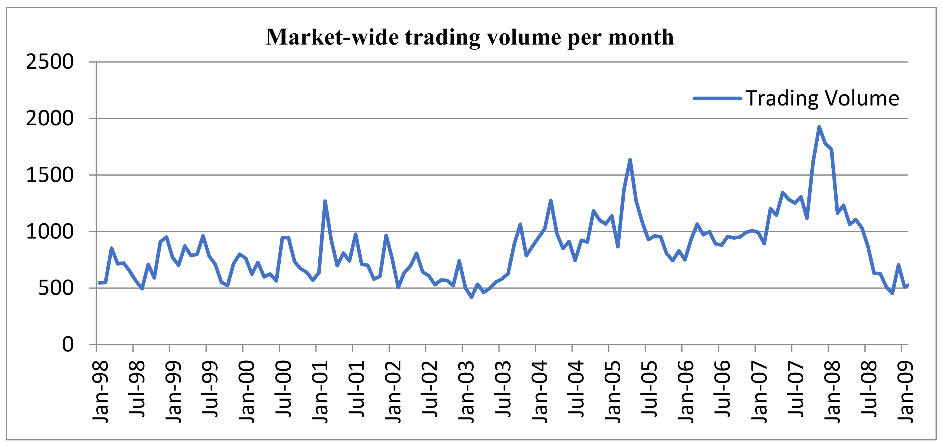
We estimate the above hedonic equations with transaction data for the urban residential market of Hong Kong: Hong Kong Island. Several characteristics of the market make it a favorable sample for our research purposes. Firstly, market liquidity and volatility are relatively high over time (see Figure 1 and Figure 2), which can greatly assist us in more closely examining the relationship between the two market fundamentals and S.A. in housing prices. Second, the market is information-efficient. In Hong Kong, all property transactions must be registered at the Land Registry of the Hong Kong government. These transaction records are available to the public around one month after sale. Property traders can draw important information about the market and the details of properties from past sales information with relative ease. An efficient market is of great empirical usefulness to vindicate the assertions of this study, which investigates the spatial phenomenon in a price discovery context. Third, the Hong Kong Island housing market is characterized by its high development density. The territory’s 80.5 ${\mathrm{km}}^2$ of landmass is dotted with as many as 5000 residential building blocks, which accommodate approximately 1.3 million habitants. Such a compact living environment enables us to observe and investigate more thoroughly the spatial dynamics of housing prices. Figure 3 presents a scatterplot of the sample residential buildings used in our analysis.

Given the efficient nature of the market, it is assumed in our models that the influence of lagged prices (WP) on current prices (P) can only last three months (i.e., m ≤ 3). Market liquidity is defined as the 3-month trading volume of the housing submarket, which is in turn defined as a space within 1000 m of the subject property, including the volume of transactions within the subject building; market volatility, as discussed, is measured at submarket level. Consistent with the treatment for lagged price and liquidity, its relevant time window is also 3 months.

Our hedonic models factor in a spectrum of structural attributes (S) for the sample housing units, including their size, floor level, building age (Age), and scale of development (SoD). Scale of development is defined as the number of housing units in the subject building. In Hong Kong, larger housing development often provides more and better facilities and amenities. SoD therefore captures the general living conditions of the housing units, and distance to the central business district is measured in meters (CBD). Their squared terms, if appropriate, are also included as independent variables; in addition, we delineate the entire sample market into 17 submarkets to proxy the neighborhood characteristics of the properties (N), and a set of time dummies measured on a monthly basis is used to capture the time effects (T).

The transaction prices, as well as the building details of the properties, are provided by a local private real estate research firm who obtain the information directly from the government on a periodic basis. The coordinates of each housing unit are collected from the Land Department of Hong Kong. In total, over 167,000 market transaction records for the period of 1998 to 2009 are employed in our analysis. The time period was in fact carefully chosen: we did not include data beyond 2009 because the selected period could symmetrically represent one whole property market cycle, with a trough occurring in 2003. In addition, the completion of new residential buildings would inevitably distort the existing spatial structure of property prices, rendering the spatial statistics less temporally comparable. Hence, the inclusion of more recent data was not statistically desirable.

We estimated the above equation with OLS methods. Since past prices can exert influence on current prices but not vice versa, statistical problems associated with endogeneity in the spatial lag terms were therefore circumvented. When error terms of the hedonic equations were independent and identically distributed, the OLS estimator was both consistent and asymptotically efficient.

Table 2. Descriptive statistics of the variables.

Variable	Unit	Mean	Std. Dev.	Min	Max
P	HKD (millions)	4.26	4.64	0.60	98.00
L*	Number of Transactions	333.00	339.07	0	3311
L**	Number of Transactions	3690.37	1202.75	1458	7114
V*	Std. Dev. (∆ price)	0.0386	0.0389	0.0006	0.3208
V**	Std. Dev. (∆ price)	0.01887	0.03494	0.00063	0.24802
Age	Year	15.16	10.94	0	59.00
Size	${\mathrm{Feet}}^2$	675.00	402.61	135.00	15,510.00
Floor	Storey	15.12	11.50	0	73.00
SoD	Unit	293.69	235.77	1	1958.00
CBD	Meter	2706.26	1430.69	249.96	9493.41

Note: P denotes property price measured in million HKD; L* denotes 3-month submarket-level liquidity; L** denotes 3-month market-wide liquidity; V* denotes 3-month submarket-level volatility; V** denotes 3-month market-wide volatility; Age denotes building age; Size denotes house size; Floor denotes floor level; SoD denotes scale of development; CBD denotes distance to center of the business district, which is assumed to be the underground train station of Central Hong Kong Island.

reports the descriptive statistics of the variables.

4. Results

Table 3. Regression Results.

Variables	Equation (2)	Equation (3)	Equation (7)	Equation (8)	Equation (9)
${\mathrm{W}}^{\mathrm{V}}{\mathrm{P}}_{\mathrm{t}-\mathrm{m}}$	-	0.0167 (0.0000)	0.0091 (0.0004)	0.0104 (0.0000)	0.0112 (0.0014)
${\mathrm{W}}^{\mathrm{H}}{\mathrm{P}}_{\mathrm{t}-\mathrm{m}}$	-	0.0184 (0.0000)	0.0141 (0.0000)	0.0264 (0.0000)	0.0230 (0.0000)
$\mathrm{L}\ast {\mathrm{W}}^{\mathrm{V}}{\mathrm{P}}_{\mathrm{t}-\mathrm{m}}$	-	-	$1.74\times {10}^{-5}$ (0.0001)	-	$2.18\times {10}^{-5}$ (0.0000)
$\mathrm{L}\ast {\mathrm{W}}^{\mathrm{H}}{\mathrm{P}}_{\mathrm{t}-\mathrm{m}}$	-	-	$1.76\times {10}^{-5}$ (0.0000)	-	$1.54\times {10}^{-5}$ (0.0000)
$\mathrm{V}\ast {\mathrm{W}}^{\mathrm{V}}{\mathrm{P}}_{\mathrm{t}-\mathrm{m}}$	-	-	-	0.3883 (0.0000)	0.4192 (0.0000)
$\mathrm{V}\ast {\mathrm{W}}^{\mathrm{H}}{\mathrm{P}}_{\mathrm{t}-\mathrm{m}}$	-	-	-	−0.1839 (0.0000)	−0.1877 (0.0000)
Constant	0.2045 (0.0000)	0.1677 (0.0000)	0.1704 (0.0000)	0.1675 (0.0000)	0.1698 (0.0000)
CBD	$-6.57\times {10}^{-5}$ (0.0000)	$-5.98\times {10}^{-5}$ (0.0000)	$-5.80\times {10}^{-5}$ (0.0000)	$-5.96\times {10}^{-5}$ (0.0000)	$-5.78\times {10}^{-5}$ (0.0000)
Age	−0.0305 (0.0000)	−0.0307 (0.0000)	−0.0307 (0.0000)	−0.0306 (0.0000)	−0.0306 (0.0000)
${\mathrm{Age}}^2$	0.0003 (0.0000)	0.0003 (0.0000)	0.0003 (0.0000)	0.0003 (0.0000)	0.0003 (0.0000)
$\mathrm{Area}$	0.0027 (0.0000)	0.0027 (0.0000)	0.0027 (0.0000)	0.0027 (0.0000)	0.0027 (0.0000)
${\mathrm{Area}}^2$	$-4.88\times {10}^{-7}$ (0.0000)	$-4.85\times {10}^{-7}$ (0.0000)	$-4.86\times {10}^{-7}$ (0.0000)	$-4.86\times {10}^{-7}$ (0.0000)	$-4.86\times {10}^{-7}$ (0.0000)
${\mathrm{Floor}}^{}$	0.0066 (0.0000)	0.0069 (0.0000)	0.0068 (0.0000)	0.0070 (0.0000)	0.0069 (0.0000)
${\mathrm{Floor}}^2$	$4.49\times {10}^{-6}$ (0.0000)	$1.67\times {10}^{-6}$ (0.0000)	$6.20\times {10}^{-6}$ (0.0000)	$3.05\times {10}^{-6}$ (0.0000)	$3.02\times {10}^{-6}$ (0.0000)
Scale of Dev.	0.0014 (0.0000)	0.0014 (0.0000)	0.0014 (0.0000)	0.0014 (0.0000)	0.0014 (0.0000)
Scale of Dev.2	$-1.59\times {10}^{-6}$ (0.0000)	$-1.59\times {10}^{-6}$ (0.0000)	$-1.60\times {10}^{-6}$ (0.0000)	$-1.59\times {10}^{-6}$ (0.0000)	$-1.60\times {10}^{-6}$ (0.0000)
Included Obs	167,418	167,418	167,418	167,418	167,418
${\mathrm{R}}^2$	0.896331	0.896594	0.896662	0.896638	0.896711
Adjusted ${\mathrm{R}}^2$	0.896169	0.896417	0.896483	0.896459	0.896531
Prob(F-Stat)	0.0000	0.0000	0.0000	0.0000	0.0000

Note: p-value in brackets.

reports the regression results for Equations (2), (3), and (7)–(9). To simplify presentation, the estimates of variables on neighborhood (N), temporal effect (T), and the contextual variation term (S* N) are intentionally left out. The full regression results are available at request. The corresponding p-value for each variable is displayed in brackets. The R-squared and adjusted R-squared for each hedonic model are also presented.

Equation (3) is essentially a traditional hedonic model with the inclusion of a spatial contextual variability variable (S* N). All coefficients were found to be correctly signed and statistically significant at the 1% level. For instance, property prices tended to decrease as distance to the CBD increased, possibly as a result of higher commuting cost. The results show that a larger apartment commands a higher price, consistent with the law of demand, with units on higher floor levels sold at higher prices, which is justifiable as they are likely to enjoy a better view, on average, or are not subject to as much pollution. Overall, this model achieves very satisfactory explanatory powers, with R-squared and adjusted R-squared at 0.8963 and 0.8962, respectively.

Transformed from Equation (3), Equation (5) adds a spatial autoregressive term, WP, to the analysis to model the price discovery process of the traders. Its coefficient suggests whether or not traders rely on prices of recently sold comparables in establishing new prices. If they do, a cobweb of spatial linkages between housing prices will be formed, inducing spatial lagged autocorrelation in housing prices. Consistent with our expectation, the housing prices were spatially autocorrelated as indicated by the positive and statistically significant coefficient on WP. Moreover, the positive coefficient implies that housing prices in the same neighborhood tended to move in tandem with each other. In other words, a higher (lower) price in one locality will generally amount to higher (lower) neighboring prices. In comparison with the results of Equation (3), we observed no material difference for the coefficients of the other hedonic variables.

Equation (7) expands the hedonic models further by including the liquidity factor (L) in the spatial processes to test H(1) and H(2). As established above, a higher market trading volume will increase vertical S.A., but the way in which it affects horizontal S.A. is less apparent, depending on how traders make use of comparables. Our results show that both ${\mathsf{\theta }}^{\mathrm{L},\mathrm{V}}$ and ${\mathsf{\theta }}^{\mathrm{L},\mathrm{H}}$ were positively signed and failed to reject H(2), but for H(1), the results were significant at the 1% level. This finding infers that traders seem to employ recently sold comparables found both within and outside the subject buildings to ascertain new prices when the market is more liquid. This may also be a manifestation of the relatively efficient nature of Hong Kong’s real estate market, where price information about properties is easily accessible in terms of time and cost. The results for the coefficients of other hedonic variables, as well as the overall explanatory power of the model, were statistically satisfactory.

Equation (8), constructed to test H(3), differed from (6) in that the liquidity variable was substituted by the volatility variable, V. The findings show that ${\mathsf{\theta }}^{\mathrm{V},\mathrm{V}}$ was positive while ${\mathsf{\theta }}^{\mathrm{V},\mathrm{H}}$ was negative at the 1% level, in agreement with our expectation that when the market is volatile, traders are inclined to put heavier weight on comparables found in the same building, and less on other comparables; hence, H(3) was not rejected. The results not only confirm the role volatility plays in the formation of S.A., but also are suggestive that housing market participants react to varying levels of market uncertainty when undertaking property valuation differently. The results for other hedonic variables were statistically satisfactory in terms of the saliency and statistical significance of their respective coefficients.

As a robustness test, Equation (9) takes into consideration the effects of both liquidity and volatility in explaining the variation of S.A. in housing prices. The results confirm our aforementioned information search conjectures in relation to the formation of S.A., which is evidenced by all coefficients displaying the expected signs and significant at the 1% level. Last but not least, we contend that since spatial autocorrelation in housing prices is not time-varying, our empirical results should remain statistically intact even if a different dataset of the Hong Kong housing market with a different time period of investigation was examined.

5. Concluding Remarks

This paper attempts to explore the determinants of spatial autocorrelation in housing prices, which is a much under-researched topic within the existing housing literature. Throughout the paper, we argue that S.A. in housing prices is a direct consequence of the price determination process undertaken by housing market participants. To verify this, we proposed three hypotheses, linking (1) market liquidity and (2) market volatility with S.A. in housing prices in a three-dimensional setting. Vertical S.A. is defined as spatial autocorrelation in housing prices for housing units located in the same building, whereas horizontal S.A. is defined as the counterpart for housing units located in different buildings. With a huge number of open market transaction data for Hong Kong, we established and statistically confirmed with the use of several spatial autoregressive hedonic models that market liquidity tends to increase both vertical and horizontal S.A. We also found that market volatility tends to increase vertical S.A. and depress horizontal S.A. Hence, we can confirm the abovementioned role that price discovery plays in the formation of, and changes in, the level of S.A. Moreover, our observation that S.A. is partially dependent on liquidity and volatility may signal that the constant S.A. assumption, which is widely accepted in the literature, should warrant closer scrutiny.

The findings of this paper reveal several implications beyond the theoretical housing literature, particularly in the areas of property valuation and the economic analysis of the housing market. Traditional hedonic models usually consist of a long list of locational variables to account for the geographical factors of real estate. If inappropriately designed, the models could likely produce spurious results. Furthermore, as elucidated by studies such as McMillen and Redfearn, 2010 [64], McCord et al., 2014 [65], and Bidanset et al., 2019 [66], geographic information systems allied with spatial–statistical approaches can better model the spatial nature of property price data, which take into consideration spatial dependence and spatial heterogeneity and help account for vertical and horizontal inequity. Against this backdrop, a more thorough conceptualization on the causes of S.A. in housing prices can prompt the development of more parsimonious yet more econometrically appealing spatial hedonic models, which can make the mass appraisal of properties much less computationally intensive and more reliable.

Further research could be undertaken to examine whether the liquidity and volatility arguments put forward in this study are empirically valid using data from other international property markets. For instance, regional housing markets within the U.K. have, over the course of the past few years, been extremely volatile, both in terms of price and return, due to political uncertainty arising from political shocks. It would therefore be worth investigating whether and how spatial autocorrelation in housing prices have changed with respect to political events in the context of price determination. In addition, the recent outbreak of COVID-19 has had a tremendous impact on almost every housing market across the globe, with trading volume plummeting given the impositions of economic lockdowns and other social distancing measures by national governments. Hence, the global health crisis could be treated as a “social laboratory” from the perspective of research, which provides an opportunity to re-validate the liquidity hypothesis postulated in this study.