Enhanced Automatic Identification of Urban Community Green Space Based on Semantic Segmentation

Abstract

At the neighborhood scale, recognizing urban community green space (UCGS) is important for residential living condition assessment and urban planning. However, current studies have embodied two key issues. Firstly, existing studies have focused on large geographic scales, mixing urban and rural areas, neglecting the accuracy of green space contours at fine geographic scales. Secondly, the green spaces covered by shadows often suffer misclassification. To address these issues, we created a neighborhood-scale urban community green space (UCGS) dataset and proposed a segmentation decoder for HRNet backbone with two auxiliary decoders. Our proposed model adds two additional branches to the low-resolution representations to improve their discriminative ability, thus enhancing the overall performance when the high- and low-resolution representations are fused. To evaluate the performance of the model, we tested it on a dataset that includes satellite images of Shanghai, China. The model outperformed the other nine models in UCGS extraction, with a precision of 83.01, recall of 85.69, IoU of 72.91, F1-score of 84.33, and OA of 89.31. Our model also improved the integrity of the identification of shaded green spaces over HRNetV2. The proposed method could offer a useful tool for efficient UCGS detection and mapping in urban planning.

1. Introduction

Green space refers to the collection of trunks, trees, shrubs, and grasses that cover the land [1]. However, not all green spaces in the city can be accessed or effectively used by residents. For example, farmland, abandoned green space, and vacant green space for construction in the city may help to generate fresh air [2], yet they could hardly contribute to social life and urbanity. In this research, we focus on ‘urban community green space’ (UCGS), defined as the green space that may foster urban public life in the city [3]. At a community level, the availability of green spaces impacts the environmental quality, helps with stress restoration [4,5], enhances the feeling of social safety [6], increases social interaction, and promotes property values [7]. Urban green space has been recognized as a key variable for assessing the livability of cities [8], whereas its spatial data at the fine-geographical scale is difficult to generate [9]. One way of obtaining the spatial information of UCGS is to extract it from remote sensing images [10]. The method of extracting urban green spaces from remote sensing images can be divided into four kinds: threshold methods, pixel-based classification methods represented by machine learning, object-oriented classification methods, and deep learning methods [11]. The threshold method selects a suitable threshold value to distinguish and extract green areas according to the difference in the spectral response of vegetation and other ground objects in one or more bands. Many threshold methods have been proposed [12,13,14,15,16,17]. However, due to the complexity of the ecological environment in urban areas and the variability of remote sensing images, it is difficult for the threshold methods to produce accurate green space contours [18]. In pixel-based methods [19,20,21,22], training pixels are selected to represent each class, and an algorithm matches the spectral properties of image pixels to the most similar and predefined class [23]. The pixel-based method realizes automatic classification but ignores the differences in spatial features between various objects, leading to confusion in recognizing similar objects. The object-oriented classification method [24,25] is the most widely used method. In the object-oriented method, the central unit of classification is no longer a single pixel, but a homogeneous object. Object-oriented classification can eliminate pixel noise and thus increases accuracy [26]. However, it is labor-intensive by heavily relying on manual intervention. The deep learning method [27] can classify objects without user intervention. It uses Convolutional Neural Networks (CNNs) [28] to intelligently mine and learn image features. Semantic segmentation is another name for the deep learning method of object extraction. Semantic segmentation assigns an object class to each pixel in a picture, allowing it to be understood at the pixel level. Unlike simple classification tasks, semantic segmentation tasks necessitate the recognition of an item and the delineation of each object’s borders. This deep learning technology offers a new intelligent interpretation strategy for the future classification of urban green spaces [29].

In recent years, using semantic segmentation to extract urban green space has become an increasing research focus. Many semantic segmentation models have been created and utilized in the field of urban green space extraction, such as Fully Convolutional Networks (FCN) [30], UNet [31], Pyramid Scene Parsing Network (PSPNet) [32], and DeepLabv3+ [33]. Some studies [34,35] have shown that the architecture with DeepLabv3+ outperform other methods by providing more smooth edge detection. Men et al. [11] proposed a novel model called Concatenated Residual Attention UNet (CRAUNet), which combined the residual structure and channel attention mechanism, and their result preserved more complete segmented edge details than UNet. According to the au- thors, CRAUNet achieved a pixel accuracy of 97.34% and a mean intersection over union (mIoU) of 94.77%. Xu et al. [36] introduced phenological features into High-Resolution Network (HRNet) model training and effectively improved urban green space classification accuracy by solving the problem of misclassification of evergreen and deciduous trees. Roberto et al. [9] used different CNN encoders on the UNet architecture to obtain urban green space polygons at the metropolitan area level. Some scholars also tried to fuse deep learning and traditional extraction methods to obtain better results. Nijhawan et al. [37] proposed a framework that combined support vector machine (SVM), local binary pattern (LBP), and GIST features with multiple parallel CNNs for feature extraction. Baoxuan et al. [38] presented a method that combines object-oriented approach with deep convolutional neural network (COCNN), with precision and kappa index coefficients being 96.2% and 0.96, respectively.

Although the studies mentioned above have made significant progress and produced promising findings for semantic segmentation in urban green space extraction, they still have limits in terms of application scale and recognition details. Firstly, prior studies and public datasets have primarily concentrated on large geographic scales, combining urban and rural areas while ignoring the precision of green space contours at fine geographic scales. Some studies [11,39] relied on typical machine learning approaches to produce training datasets rather than exact hand annotation. Furthermore, publicly available high-resolution remote sensing image datasets, such as the Gaofen Image Dataset (GID) [40], ISPRS Potsdam [41] and ISPRS Vaihingen [42], mapped and evaluated many feature types at large sizes from a macro perspective. Green space classifications were ignored in their databases, and rural and urban areas were jumbled together [43]. Secondly, small objects and the green spaces covered by shadows often suffer misclassification. Small, scattered, or shadowed green spaces were frequently omitted in the presentation of the results of most studies [36,39,44,45,46], while fields, playgrounds, or barren meadows were frequently misclassified. The main reasons for the second problem are two characteristics of green spaces: the variety of green space types and the integration of green space boundaries with the context. Unlike other ground objects, the types of UCGS are diverse, multi-scale, and highly fragmented [11]. For example, UCGS can range from small sidewalk greenery to large-scale parks. As green spaces have highly irregular contours [47], it is difficult to distinguish the precise outline of a green space when its irregular contours are confused with a complex background, such as shadows.

To address the first issue, this work used publicly accessible high-resolution remote sensing images to generate a dichotomous dataset concentrating on urban community green space (UCGS) at a neighborhood size. We discriminated between urban and non-urban areas before making detailed hand annotations on urban community green spaces. In comparison to other studies, this work focuses mainly on urban regions. For the second issue, this work developed a segmentation decoder for HRNet that has two auxiliary decoders. When the high- and low-resolution representations are merged, our proposed model adds two branches to the low-resolution representations to improve their discriminative capabilities, resulting in improved overall performance. To evaluate our strategy, the proposed framework was applied to four different regions of Shanghai, China. The following three aspects are the key contributions of this paper:

• We produced an open UCGS semantic segmentation dataset. UCGS in shadows is identified in the dataset for better extraction;
• We proposed a method that automatically screened urban communities from remotely sensed images. Our method improved efficiency in avoiding misclassified rural fields;
• We developed a segmentation decoder with two auxiliary decoders for HRNet to improve the overall performance of urban community green space extraction.

2. Methods

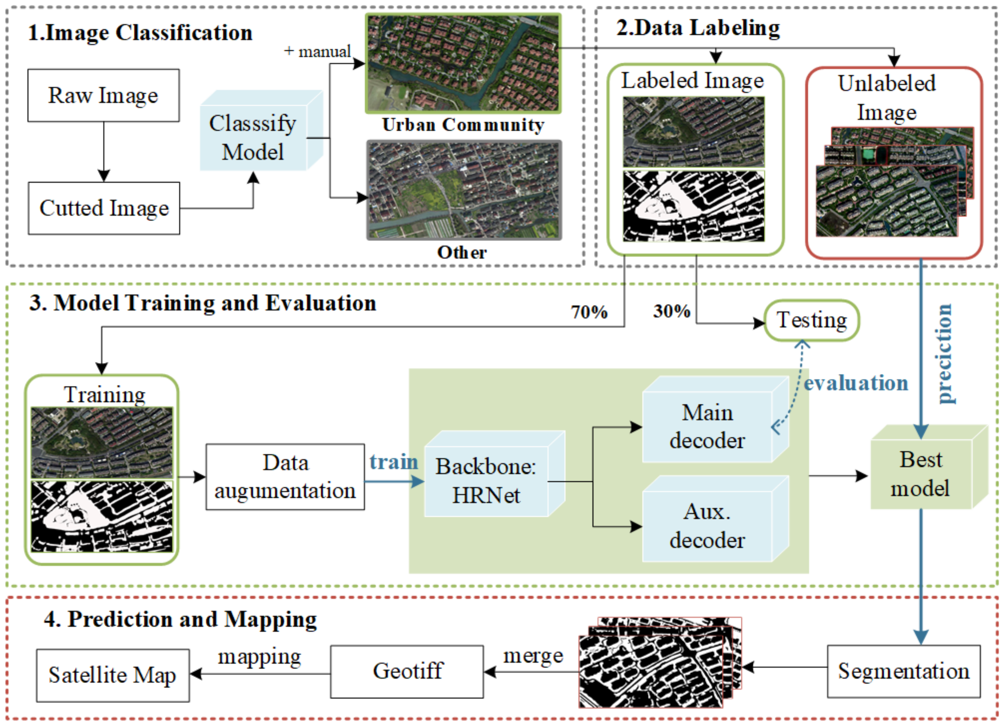
2.1. The Overall Workflow

Figure 1 depicts the overall process flow. There are four parts to the process: (1) image classification for urban communities; (2) data labeling; (3) deep learning model training and evaluation; and (4) prediction and mapping.

In the image classification stage, images containing UCGS were filtered out for subsequent labeling. This operation allowed the substantial exclusion of fields that do not contain UCGS. In the data labeling stage, we created a labeled dataset with marked UCGS. Note that UCGS covered by shadows were labeled deliberately. In the model training and evaluation stage, the image was extracted by the HRNet backbone to get the feature map. The featured map was then segmented after the proposed decoder. In the prediction and mapping stage, UCGS were identified in the raw images and mapped back onto the satellite map.

2.2. Image Classification

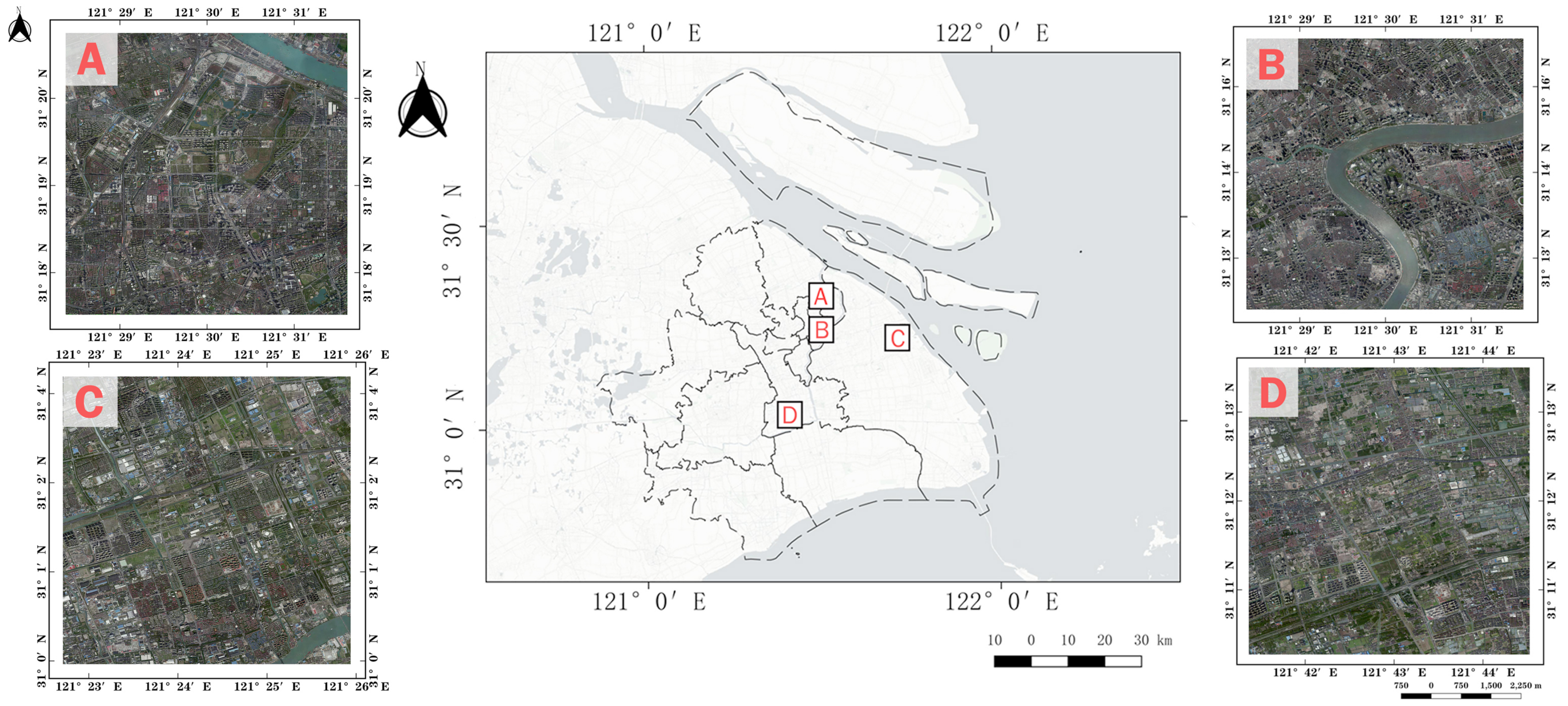
2.2.1. Study Area and Data Sources

The case city, Shanghai, has set the goal to become a more ecologically integrated and livable city in its latest master plan [48,49]. According to the Shanghai Statistical Yearbook, Shanghai’s urban green space has grown to 157,785 hectares, accounting for 39.7% of the city’s total land area [50]. In October 2021, the Shanghai satellite map was obtained from Map World [51] via 91 Satellite Image Assistant [52]. The National Platform for Common Geospatial Information Services [53] and the Shanghai Surveying and Mapping Institute [54] provided the map of Shanghai subdistrict. There are three red-green-blue bands in all of the data, with a spatial resolution of about 0.51 m. We chose four representative regions to evaluate and compare the model predictions, as shown in Figure 2, because the distribution of green space in Shanghai changes with building density [55,56,57].

Table 1. Detailed data description.

Name	Satellite	Location	Acquisition Date	Area (km2)
A	GF-2	Baoshan District and Yangpu District	2021/10/5	41.23
B	GF-2	Huangpu District and Pudong New Area	2019/11/9 & 2021/11/19	41.23
C	GF-2	Pudong New Area	2018/4/10 & 2021/10/23	41.23
D	GF-2	Minhang District	2020/5/3	41.23

shows the specific details for each region.

2.2.2. Classify Urban Community Images

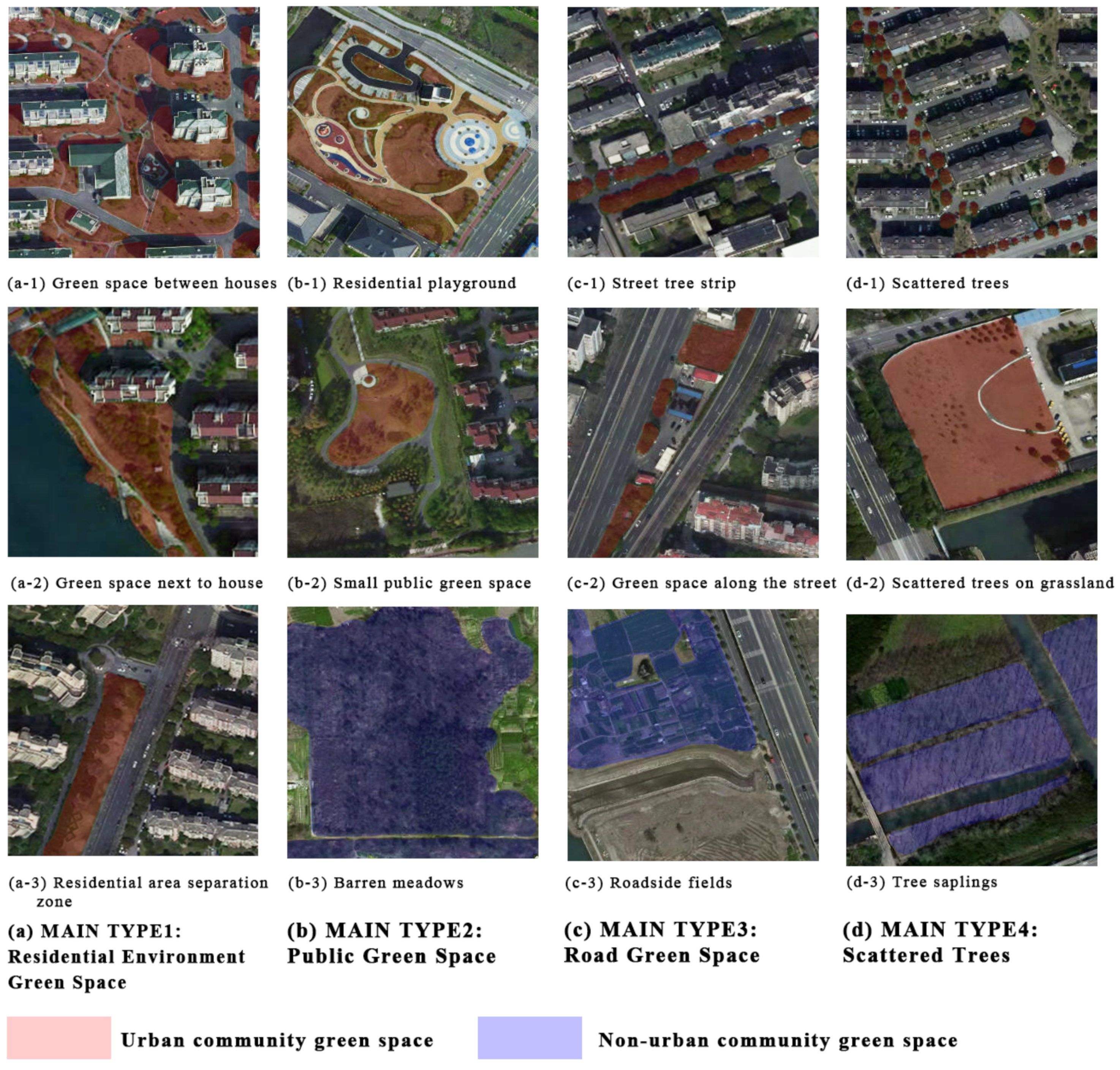
Raw images from Map World were cut uniformly to 38,850 images of 512 × 1024 pixels patches with non-overlapping grid partition. A simple ResNet-18-based classifier was built to filter out images containing communities. This classifier used 1000 artificially screened True and False samples as the training dataset and another 1000 samples for testing. This classifier had 99.1% accuracy on the testing dataset. With the help of the classifier and a little manual work, we obtained 7023 urban community images for subsequent labeling, model training, and mapping.

2.3. Data Labeling

A considerable amount of high-quality and fine-grained labeled data is required to train a semantic segmentation model [11], and existing open-source datasets were not explicitly built for green space classification at a community size. Therefore, we created a dataset with urban community green space labels manually. A total of 1000 images from 7023 urban community images were randomly picked and labeled using the labelme tool [58].

The Ministry of Housing and Urban-Rural Development of the People’s Republic of China (MOHURD) [59] released the national garden and park urban standard in the year 2000 [60]. We focused on urban green spaces that are closely linked to people’s daily lives, and made a more detailed and precise classification of urban community green spaces according to the document. Figure 3 shows examples of UCGS, including green space between houses (a-1), green space next to houses (a-2), residential area separation zones (a-3); public green space including residential playgrounds (b-1), small public green spaces (b-2); road green spaces including street tree strips (c-1), green spaces along the street (c-2) and scattered trees (d-1, d-2). It is important to note that UCGS does not include barren meadows (b-3), roadside fields (c-3), or tree saplings (d-3).

The final labeled dataset was stored as 8-bit ground truth binary label. Further, 60% of the dataset was selected for training, 10% was used for evaluation validation during training, and the remaining 30% was reserved for testing the performance of the trained model. There was no overlapping among the training, validation, and testing datasets.

2.4. Model Training and Evaluation

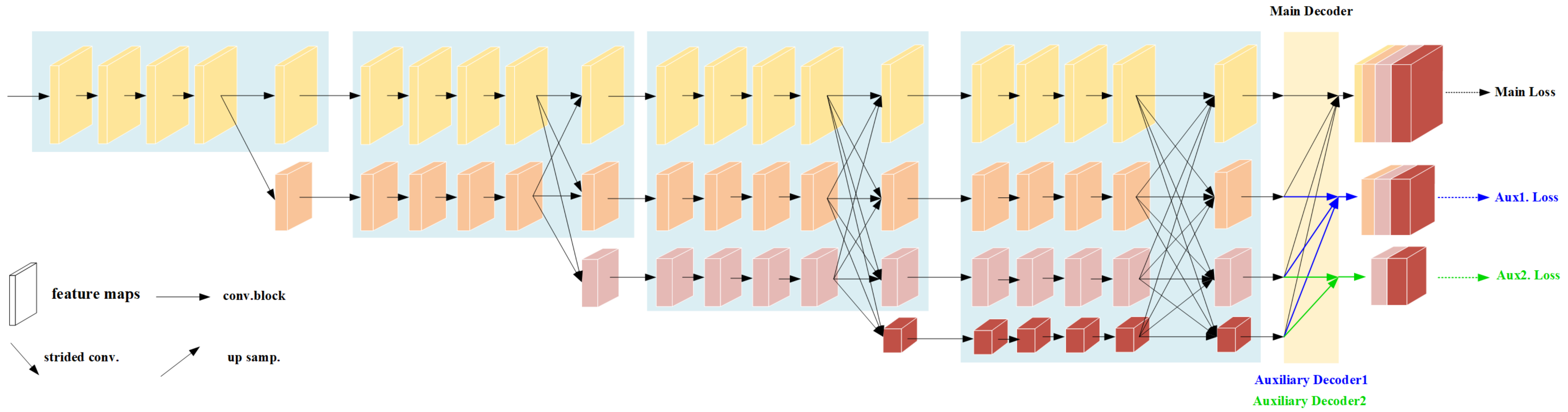
2.4.1. Network Structure

We now introduce auxiliary learning for HRNet, a proposed approach for automatically recognizing UCGS (aux-HRNet). We added two auxiliary decoders to the low-resolution representations to improve their discriminative ability, as inspired by the extensive deep supervision literature [61,62,63] and GAN-based literature [64,65]. This improved the overall performance when the high- and low-resolution representations were fused. The proposed network structure is depicted in Figure 4 as an overview. An HRNet backbone, a combination decoder with two auxiliary decoders and the main decoder make up this model. The code and model are publicly available at https://github.com/ChenJiangxi/aux-HRNet-for-UCGS (accessed on 6 June 2022).

2.4.2. HRNet Backbone

We used HRNet (High-Resolution Network) [66] as our backbone in semantic segmentation in this paper. HRNet joins high-to-low convolution streams in parallel, as shown in Figure 4. By repeatedly fusing the representations from multi-resolution streams, it maintains high-resolution representations throughout the process and provides dependable high-resolution representations with good position sensitivity.

The higher the level of semantic information in a feature, the better the discriminative capacity, at the expense of resolution. Shallow features have high resolution, but they do not have a lot of semantic information. However, HRNet’s high-resolution representation is not only semantically sound, but also spatially accurate. These benefits stem from two factors. First, instead of joining the high-resolution and low-resolution convolutional streams in series, HRNet joins them in parallel. As a result, HRNet may sustain high resolution rather than recovering high resolution from low resolution, implying that HRNet’s learning process is more spatially precise. Second, HRNet repeats multi-resolution fusion in order to improve high-resolution representations using low-resolution representations and vice versa. As a result, all representations from high to low resolution are semantically stronger.

The existence of high-resolution maps improves the spatial accuracy of the feature maps. Furthermore, the inclusion of low-resolution maps results in richer higher-level semantic properties, but the target locations are coarser. The semantic segmentation problem requires both low-level details and high-level semantics [67]. In the task of extracting green spaces, geographical precision can improve the accuracy of the green spaces recognized, while semantic enrichment improves the capacity to identify green spaces. We believe that the misclassification problem, which is more important than the problem of poor spatial accuracy, should be given greater attention when extracting green spaces.

2.4.3. Main Decoder and Auxiliary Decoder

HRNetV2 [66] was originally proposed for semantic segmentation by estimating segmentation maps from a combined high-resolution representation. In Figure 5a, HRNetV2 is adopted as the main decoder in training and inferencing. The method of HRNetV2 is as follows: (1) rescale the low-resolution representations through bilinear upsampling without changing the number of channels to high resolution; (2) concatenate the (upsampled) representations from all the resolutions; (3) a $1\times 1$ convolution mixes the four representations and gains the feats; (4) the loss is calculated by comparing the classification results obtained from feats by $1\times 1$ convolution with ground truth.

Our two auxiliary decoders are shown in Figure 5b,c. The construction of the auxiliary decoders was the same as HRNetV2, but different feature map inputs were employed. The three low-resolution subnets output from the fourth stage of HRNet were used as input for the auxiliary decoder in Figure 5b. To obtain feats, they were also upsampled and concatenated, followed by convolution $1\times 1$. Two deeper low-resolution subnets were given to the auxiliary decoder in Figure 5c. Furthermore, the classification maps produced by the three decoders did not have the same height and width (channel number = number of classes for all three). When compared to the ground truth, they were resized using bilinear upsampling to the same size as the ground truth, and then the loss was computed.

The main decoder head and auxiliary decoder heads were used in parallel. Auxiliary learning aims to achieve deep supervision, a well-known technique for improving performance [68]. The auxiliary decoder aids in learning optimization and was removed during the inference phase [69]. Therefore the extra auxiliary decoders did not increase the inference cost. By adding an auxiliary decoder to the HRNet backbone’s low-resolution subnets, we can improve the low-resolution subnets’ classification performance, making their semantic information more accurate. As a result, by fusing features with the low-resolution feature map, the high-resolution feature map can obtain more accurate semantic information, boosting the high-resolution feature map’s discriminative capabilities.

2.4.4. Online Hard Example Mining

Generally, the number of background pixels is substantially larger than the number of foreground pixels in segmentation tasks. A similar imbalance problem existed in our sample as well. The data imbalance issue could result in decreased training efficiency and accuracy. To overcome the problem, we used the Online Hard Example Mining (OHEM) algorithm [70]. The OHEM algorithm’s main idea is to filter away hard data that have a large impact on classification based on the loss, and then apply the filtered samples to stochastic gradient descent training. OHEM works nicely in the Stochastic Gradient Descent (SGD) paradigm, simplifies training by eliminating several heuristics and hyperparameters, and may result in improved convergence (less training set loss) [70].

2.4.5. Loss Function

In semantic segmentation, the loss function metric is an algorithm that evaluates the difference between training prediction and ground truth labels. The model can attain the convergence stage and reduce prediction error by minimizing the loss function. To establish the best appropriate loss function metric for our data, we looked at their spatial properties. UCGS may only represent a small percentage of pixels because most cities are covered by built-up regions populated by roadways, buildings, and other impermeable surfaces. This design results in a class imbalance, which may lead to errors and a bias toward the background class, which covers the majority of the region of interest. Deep learning-based semantic segmentation research [71,72,73] has shown that the Dice Loss [74] is an adequate loss function for the imbalance problem. Equation (1) is used to compute the Dice loss.

$$\mathrm{Dice}\mathrm{Loss}=1-\frac{2|I_{GT}\cap I_{SEG}|}{|I_{GT}|\cup |I_{SEG}|},$$

(1)

where $I_{GT}$ is the input ground truth, and $I_{SEG}$ is the output segmentation. A Dice Loss of 1 indicates no overlap between prediction and ground truth, whereas a value of 0 means that the prediction overlaps the labeled ground truth [75]. When it comes to the target and auxiliary losses, we normally employ the same dice loss, but they can also be different. Therefore, the total loss during training can be calculated as Equation (2). To attain the optimum model performance, we tweak $\alpha$ and $\beta$ in (0, 1) in our method.

$$L=L_{target}+\alpha L_{aux1}+\beta L_{aux2}.$$

(2)

2.4.6. Parameters for Evaluation

In this study, five evaluation indexes were selected to evaluate the performance, including Precision, Recall, the intersection over union (IoU), F1-Score, and overall accuracy (OA). The precision indicated the proportion of the true UCGS to all the UCGS identified by the model, representing the model’s accuracy. In contrast, the recall indicated the proportion of the true identified UCGS to all the UCGS in the given samples, reflecting the model’s capability of discovering the true UCGS. IoU is the ratio of the intersection and the union of the ground truth and the predicted area. F1-Score, also known as the balanced score, is defined as the harmonic average of precision and recall rate. It is a common evaluation index for semantic segmentation. Overall Accuracy (OA) is a comprehensive evaluation index of classification results and represents the probability that the classification result for each pixel is consistent with the actual type of the label data. These evaluation metrics are computed between the predicted UCGS and the ground truth. The calculation equations for the indicators are shown in

Table 2. Evaluation metrics. TP FP FN and TN are the true positive, false positive, false negative, and true negative classifications, respectively. N represents the total number of pixels. The first four metrics are used only for the UCGS category.

Accuracy Evaluation Criteria	Formula
Precision	Precision $=\frac{\mathrm{TP}}{\mathrm{TP}+\mathrm{F}}$
Recall	Recall $=\frac{\mathrm{TP}}{\mathrm{TP}+\mathrm{FN}}$
IoU	IoU $=\frac{\mathrm{TP}}{\mathrm{TP}+\mathrm{FP}+\mathrm{FN}}$
F1-score	F1-score $=2\times \frac{\mathrm{Precision}\times \mathrm{Recall}}{\mathrm{Precision}+\mathrm{Recall}}$
OA	OA $=\frac{\mathrm{TP}+\mathrm{TN}}{\mathrm{N}}$

.

2.5. Prediction and Mapping

Following the identification of the best performance model, it was utilized to predict the UCGS on the satellite picture, and the UCGS was then mapped to obtain high-quality UCGS distribution in Shanghai. The model outputs in this work are binary classes at the pixel level (UCGS and non-UCGS). Non-UCGS pixels were removed, and all of the outputs were recombined in raw image size. We were able to achieve a one-to-one connection between raw images and prediction findings in this method. We used the open-source geographic information system QGIS [76] to visualize the precise geographic projection of the projected results. The original raster data is raw images with the exact geographical coordinates of each corner. The expected findings are projected on the WGS 84 (EPSG:4326) coordinate reference frame using the Georeferencer tool [77].

3. Results

3.1. Experimental Settings

3.1.1. Implementation Details

The entire procedure was implemented in the semantic segmentation framework, mmsegmentation [78].

With a batch size of 2, all models were trained for 80k iterations. The detailed configuration of model training parameters is described as follows. The optimizer is Stochastic Gradient Descent (SGD). The initial learning rate and momentum parameters were set as 0.01 and 0.9, respectively. The learning rate was annealed during training using the poly learning rate policy, in which the base learning rate was multiplied by $1-{\left(\frac{iter}{max\_iter}\right)}^{power}$ with power = 0.9 at each iteration. The training process was carried out on an NVIDIA GeForce RTX 2060 GPU, 6 GB of RAM, using Python 3.8, PyTorch deep learning framework, accelerated by cuDNN 10.1.

The data augmentation techniques are adopted to increase the size of training dataset [79], add more variability to it and reduce the “overfitting” of deep CNN caused by limited training samples [80]. We use random crops of size 256 × 512 and apply random rescaling in the range [0.5, 2.0], random horizontal flip, and photometric distortion to our dataset. All training processes used the OHEM algorithm, with only pixel-valued values with confidence scores below 0.7 being used for training.

3.1.2. Models for Comparison

Fully Convolutional Networks (FCN) [30], UNet [31], Pyramid SceneParsing Network (PSPNet) [32], Deeplabv3 [81], DeepLabv3+ [33], and HRNet [66], as well as pixel-based categorization approaches such as Maximum Likelihood (ML) and Random Forest (RF), are compared to the proposed model’s performance.

The encoder used in the Deeplabv3+, Deeplabv3, PSPNet, and FCN experiments is a ResNetV1c-50 [82] pretrained on ImageNet [83]. ResNetV1c replaces the 7 × 7 conv. in the input stem with three 3 × 3 convs [84], as opposed to default ResNet (ResNetV1b). We used the multi-scale feature mosaic method of HRNetV2 suggested in the work [66] for the HRNet. The width C of the high-resolution subnet in the last three stages of the HRNet-W48 backbone was 48, whereas the widths of the other three parallel subnets were 96, 192, and 384, respectively. The width C of the HRNet-W18 backbone is equal to 18, accordingly. For inference on test dataset, we use the model that performed best during the training phase. We obtained metrics for all deep learning methods.

We utilized these classifiers on Arcmap of ArcGIS 10.7 [85] for the ML and RF approaches. To distinguish the green spaces from the other objects, the first step was to select a specific section of the image. The Random Forest Classifier and Maximum Likelihood Classifier were then used to train the annotated picture and generate the classifier model. The classifier model was used to predict the results of the remaining satellite photos in the third stage. The maximum number of trees in the random forest classifier was 50, the maximum tree depth was 30, and the maximum number of data per class was 1000. Finally, the images with the projected green space were obtained.

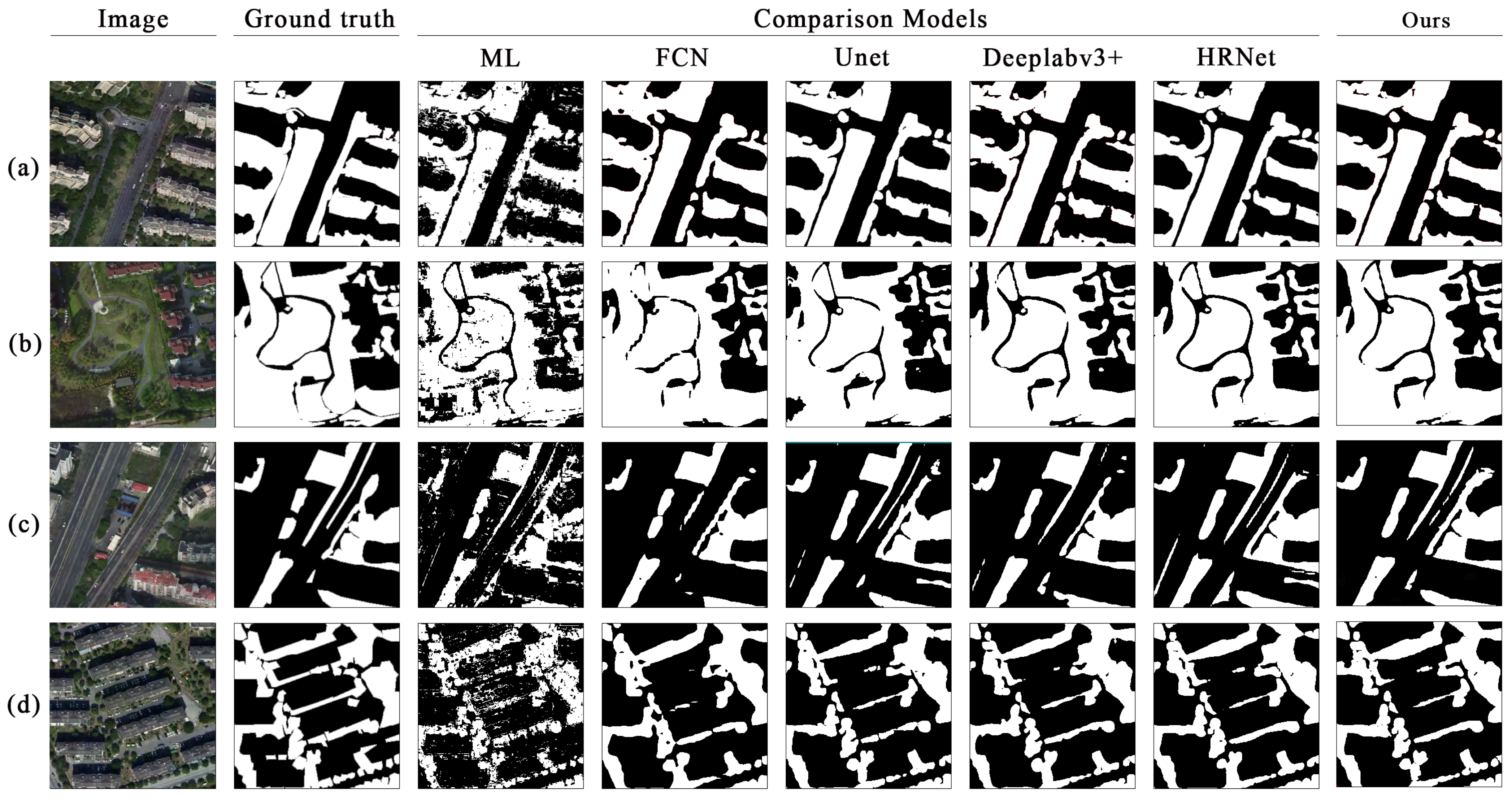
3.2. Comparison of Different Classification Methods

We conducted various comparative experiments to verify the effectiveness of our proposed technique.

Table 3. Performance of different classification methods.

Method	Backbone	Precision	Recall	IoU	F1-Score	OA
HRNetV2	HRNet-W48	82.05	85.76	72.21	83.87	88.92
HRNetV2	HRNet-W18	78.58	88.92	71.57	83.43	88.14
FCN	Unet	82.91	84.44	71.92	83.67	88.93
Deeplabv3+	ResNet-50	84.81	82.04	71.53	83.4	89.03
Deeplabv3	ResNet-50	84.14	82.13	71.11	83.12	88.8
FCN	ResNet-50	81.2	85.33	71.25	83.21	88.44
PSPNet	ResNet-50	83.47	81.39	70.1	82.42	88.34
Maximum Likelihood	-	70.56	75.75	57.26	72.33	61.69
Random Forest	-	64.89	82.23	56.26	71.48	79.1
Ours	HRNet-W48	83.01	85.69	72.91	84.33	89.31
Ours	HRNet-W18	84.46	83.3	72.23	83.88	89.24

shows how all of the approaches performed on the test dataset. In addition, we chose specific urban green space regions to better understand the reasons for the table’s accuracy discrepancies. Figure 6 depicts segmentation results from various semantic segmentation networks in various types of urban community green spaces.

Deep learning approaches exhibited fewer errors and omissions than the Maximum Likelihood (ML) and Random Forest (RF) methods, as demonstrated in Figure 6. The ML and RF classification algorithms were unable to reliably determine the boundary of different urban green space categories, where the phenomena of misclassification and omission was evident. For example, in Figure 6, the Maximum likelihood (ML) technique consistently classifies the shaded part of the road of the image as green space while missing the shaded part of the green area. There are two basic causes for this problem. The first is the limitation of the classifier’s performance. Another is the difficulty of distinguishing objects, which is due to the complexity of greenfield colors in remote sensing images, such as “the same object in different colors” and “foreign objects in the same color” [36].

Deep learning methods, on the other hand, produced outputs that always had clear boundaries and performed better than ML and RF. Various deep learning models also produced different training results. In addition to our own model, HRNet outperformed other models in terms of evaluation metrics, resulting in better classification results. This result was in line with the findings of the article [36]. Based on the experimental findings, the following conclusions can be drawn: (1) The segmentation results from FCN were skewed. The jagged outlines of the public green space in Figure 6c caused the road to be misclassified as a green space, which can be explained by the FCN network structure upsampling process’ limitations. This results in severe detail loss in the images; (2) UNet was only second to HRNet in terms of performance. Although UNet’s classification results were far superior to FCN’s, there was still misclassification of roads in Figure 6c and omission of trees in Figure 6b; (3) as seen in Figure 6b, DeepLabv3+’s results frequently misidentify green regions that are obscured by shadows.

The classification ability of the model in this paper was the best. In terms of evaluation metrics, our model outperformed HRNetV2 with the HRNet-W48 backbone by 0.7 points in IoU, 0.46 points in F1-score, and 0.39 points in OA. Even when compared to HRNetV2 with HRNet-W18 as the backbone, our method outperformed it. Our model reduced misclassifications in terms of classification outcomes. For example, HRNet misclassified a road as green space in Figure 6c, whereas our classification results have no such problem. The auxiliary segmentation decoder, in addition to the main segmentation decoder, contributed to our model’s excellent performance. By adding two auxiliary decoders in training, the model in the paper paid greater attention to low-resolution subnets with richer semantic information than HRNetV2. When multi-resolution subnets exchange data, low-resolution feature maps can contribute more accurate semantic information to high-resolution subnets, thereby boosting the accuracy of high-resolution representations.

Our trained model is publicly available at https://drive.google.com/file/d/1spQj1_3cXPcVyH36vUbdrmCiwhfQItP5/view (accessed on 6 June 2022) for other scholars to perform transfer learning when studying similar problems.

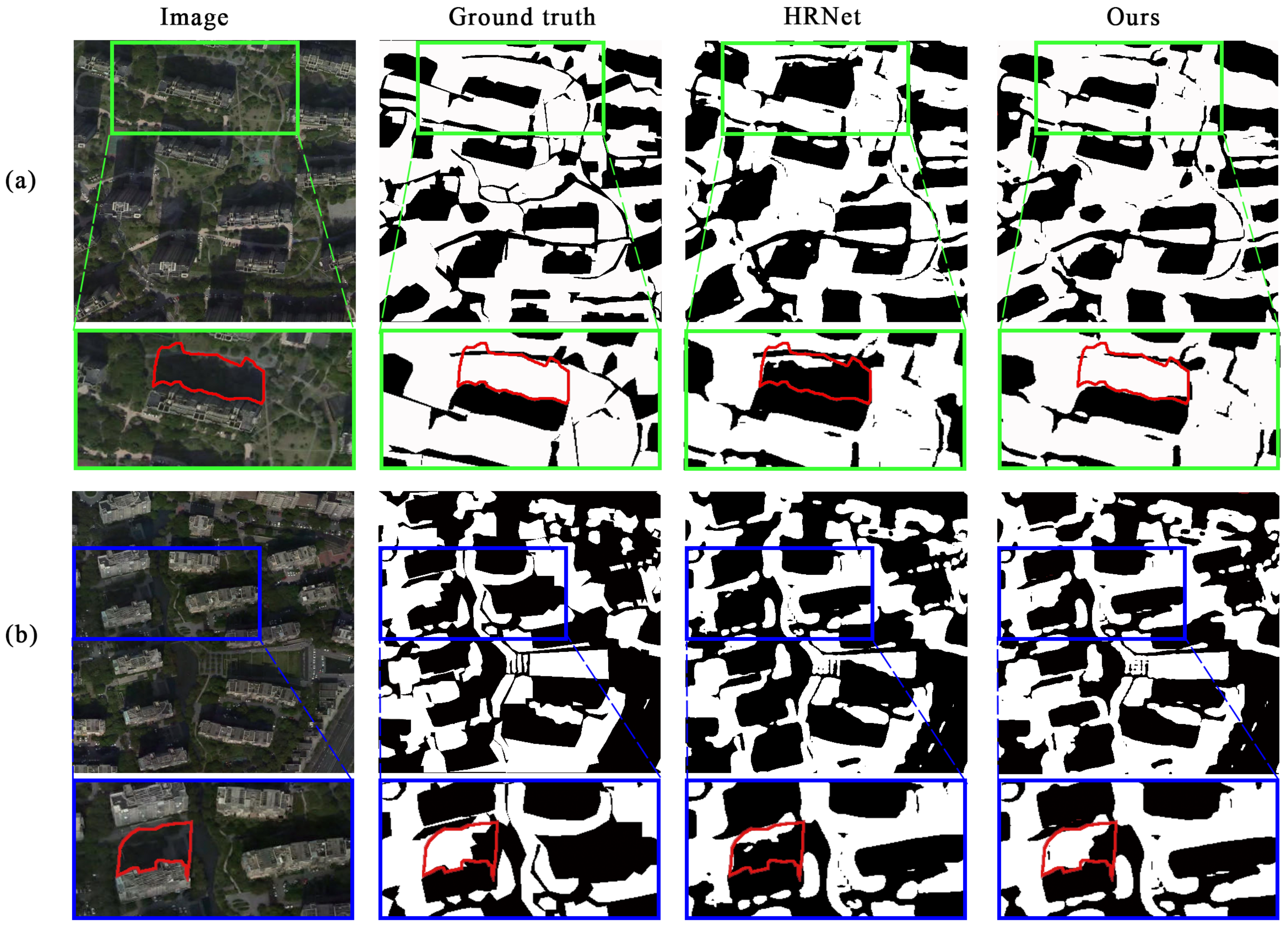
3.3. Improvement on the Classification of Urban Community Green Space in Shades

This paper tried to improve the identification of green spaces covered by shadows. The following are some of our efforts: (1) In our dataset, we deliberately labeled green regions that were obscured by shadows; (2) We improved the accuracy of the model’s advanced semantic information, thus enhancing the model’s overall recognition capability.

As seen in Figure 7, our model performed significantly better than HRNet in identifying shaded green patches. In Figure 7, for example, the green area surrounding high-rise housing is frequently obscured by the shadows of high-rise structures. The shaded green space behind the building was recognized by our approach in Figure 7a, whereas the HRNet misclassified the shade as a non-UCGS. In Figure 7b, HRNet only identified a portion of the shaded green space. Our approach, on the contrary, recognized the full green space. Despite the fact that our model didn’t entirely detect the outline of green patches obscured by shadows, it was a significant improvement over HRNet.

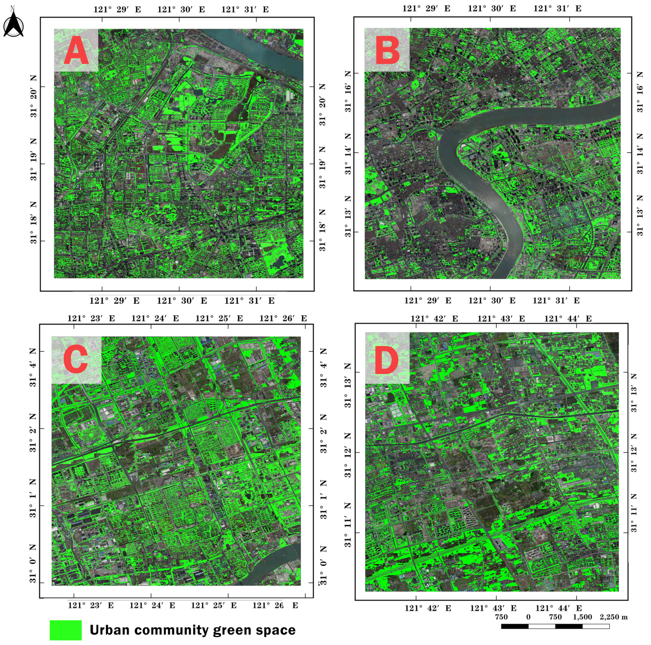
3.4. Green Space Distribution of the Sampled Areas

As is illustrated in Figure 8, green space was mapped on four representative study areas with a high density of urban communities, including downtown and suburban region. Area A is mainly located in Baoshan district. The land cover of Baoshan district is predominantly residential communities, including some urban green spaces and parks. It is worth noting that the barren meadow in the green space in the up-right corner of area A was not mistaken for green space, which verifies the accuracy of our model. Area B represents the business area and covers the busiest area of Shanghai, including the Bund and part of Huangpu River. The shadows of the tall buildings covering part of the green space in these regions add to the difficulty of our task, which is also an unresolved problem for many traditional methods of green space classification. However, taking the center area of B featuring long and large-scale shadows as an example, our model precisely identified the green space surrounded by tall buildings with shadows on it. Area C is located in Minhang District, a typical industrial area with many communities. It is clear that green vegetation on the roofs and the green plastic playgrounds in schools are not misidentified as green space using our model. Area D, situated in Pudong new area, has relatively large farmland areas, so it stands for the agricultural area. Our model succeeded in distinguishing farmlands from the residential green space that we are interested in, making it also possible to be used in extracting community green space in suburban regions.

The applications of our approach to various settings, such as residential areas, commercial areas, industrial regions, and agricultural areas, have proven its effectiveness for extracting urban community green space, based on the analyses above.

Figure 8 also shows that different areas of Shanghai have an uneven distribution of green spaces, the exact value of which can be found in

Table 4. Percentage of UCGS of the four areas.

Area	A	B	C	D
Percentage of UCGS	19.00%	12.14%	22.32%	21.62%

. The less green space there is the closer you get to the city core, and the more fragmented it becomes. Region B, for example, has the least quantity of green space of the four. The most UCGS are found in Region C, a freshly created industrial area with several villages. The recently created Pudong (right side of the river) has more green space than the Puxi area (left side of the river) in Region B, which is closer to the city center. It suggests that the planning of new cities takes into account green space more than the planning of ancient city centers.

4. Discussion

Semantic segmentation studies using similar approaches to map urban green space [9,11,36] reported F1-score of 96.32, 57.48, and 84.02, respectively. The result in this study is 84.33, which is slightly higher than that in the paper [36]. The referenced studies focus on larger scale identification and do not consider the details of scattered trees and the identification of shaded green spaces; however this research seeks to more accurate identification at fine geographic scales. Although it is a small improvement over HRNet, our approach applied deep supervision to HRNet and improved model performance with only two additional auxiliary decoders. From the visualization results, our model can distinguish between field and community green spaces, and performs better on shaded green spaces. The proposed method could offer a useful tool for efficient UCGS detection and mapping in urban planning, and provide a model of UCGS data extraction for studies focusing on urban design and resident health.

Further, we have a deep discussion of our proposed model.

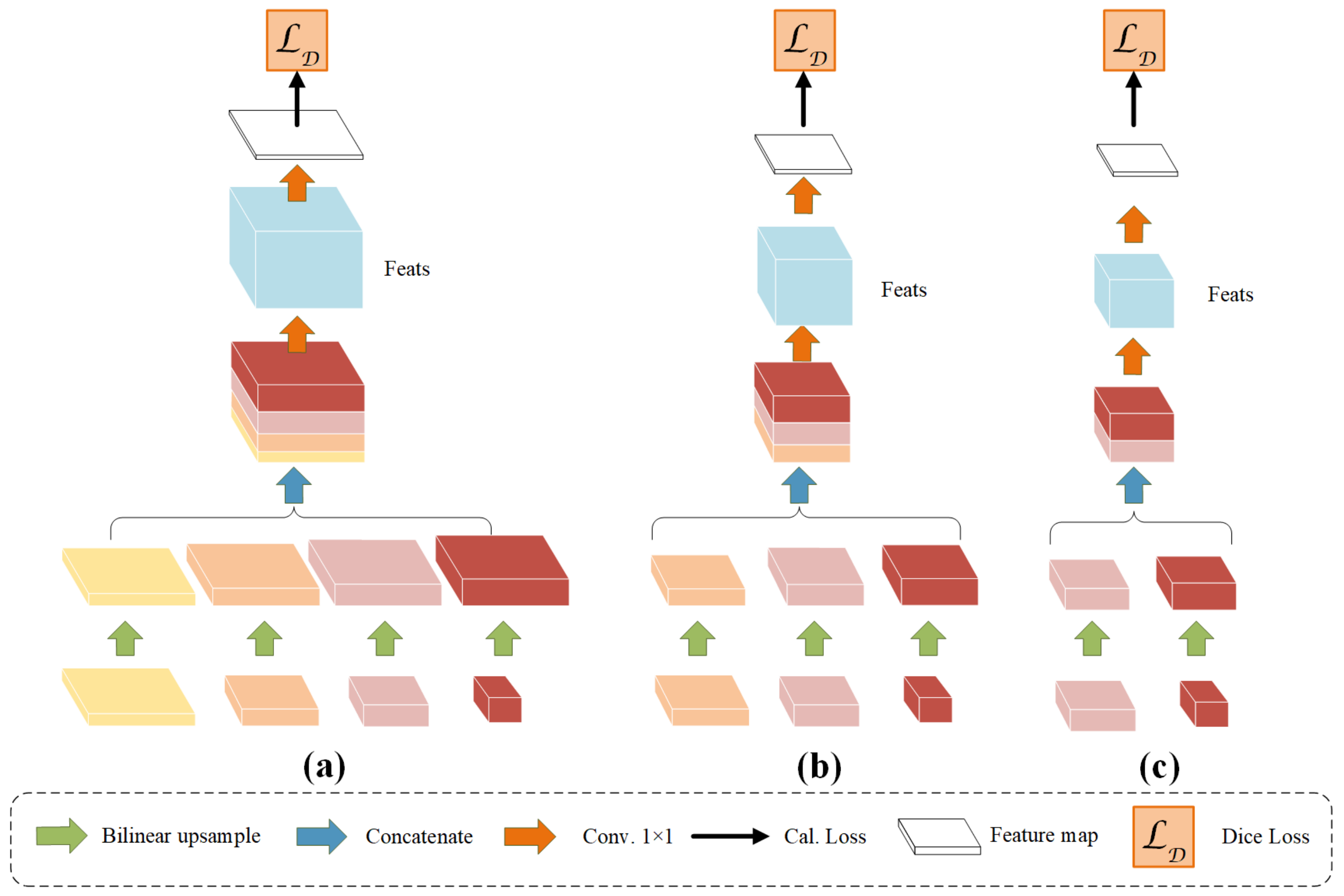
4.1. Different Input Combinations for Auxiliary Decoder

Since the HRNet backbone outputs four feature maps with different resolutions, we explored how the combination of different feature maps with the auxiliary decoder impacts the performance of detecting green space. In descending order of resolution, we set the series of feature maps output by the HRNet backbone to $f_1,f_2,f_3,f_4$. According to the paper [66], the accuracy of prediction outcomes in semantic segmentation rapidly drops from high-resolution feature map $f_1$ to low-resolution feature map $f_4$.

HRNet networks were initialized using the model pre-trained for ImageNet classification. In the following experiment, all auxiliary loss weights are equal to 0.4.

Table 5. Model performance of the auxiliary head with different combinations of feature maps, where 🗸 means that the feature map is used as input to the decoder.

Comb.	Aux.	Feature Map				IoU	F1-Score	OA
		${\mathit{f}}_{\mathbf{1}}$	${\mathit{f}}_{\mathbf{2}}$	${\mathit{f}}_{\mathbf{3}}$	${\mathit{f}}_{\mathbf{4}}$
(a)	aux1	🗸	🗸	🗸		72.42	84.01	88.97
(b)	aux1	🗸	🗸	🗸		71.97	83.7	89.1
	aux2	🗸	🗸
(c)	aux1		🗸	🗸	🗸	72.16	83.83	88.76
(d) (Ours)	aux1		🗸	🗸	🗸	72.91	84.33	89.31
	aux2			🗸	🗸

summarizes the results of the four possible combinations. According to the comparison, the combination (d) (ours) has the best performance. With one auxiliary decoder with $f_2,f_3,$ and $f_4$ as input, the combination of two decoders was 0.75 points greater than combination (c). However, increasing the number of auxiliary decoders does not always improve the model’s performance. Combination (b), for example, does not perform as well as combination (a). If the auxiliary task is closely related to the main task, it can be useful, according to the article [86]. As a result, the performance is affected by the degree to which different resolution feature maps are evaluated.

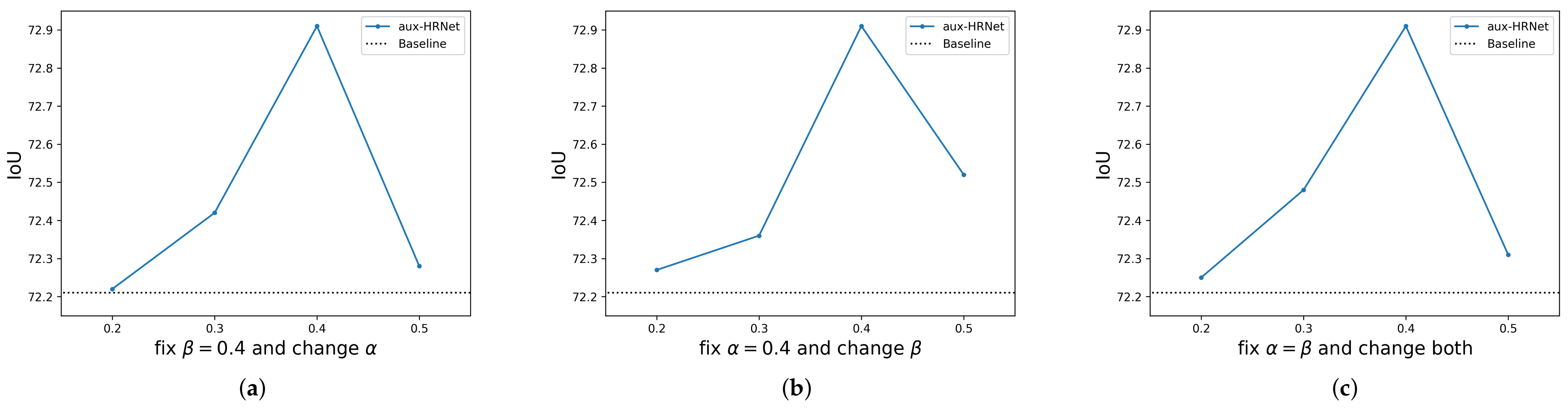
4.2. Different Weights of Auxiliary Learning

We designed three experiments to see how the weight of the auxiliary task affected the overall task and the primary task. The weights of the losses created by the two auxiliary decoders in the total task, according to Equation (2), are $\alpha$ and $\beta$. We first set $\beta$ equal to 0.4, then varied the value of $\alpha$ and watched the trained model’s performance. Figure 9a depicts the result. We also fixed $\alpha$, changed $\beta$, and did the same comparison experiment. The result is shown in Figure 9b. Figure 9c depicts the result of setting $\alpha$ equal to $\beta$ and modifying both of them at the same time. All of the experimental results suggest that the weight of the auxiliary task has an impact on the model’s performance. Regardless of the weights, aux-HRNet outperforms the methods without auxiliary learning. Appropriate weights for the auxiliary tasks should be chosen when utilizing the aux-HRNet model for various activities.

4.3. Influences of Training Tricks

The impact of the following key training strategies [87] on model performance was investigated. (1) OHEM, which can promote the model training by increasing the proportion of difficult samples in total loss; (2) one of the most used augmentation approaches, random rescale, can improve the models’ generalization capacity and scale diversity. We used random crops of size $256\times 512$ in the experiment and applied random rescaling in [0.5, 2.0] and only pixel-valued points with confidence scores below 0.7 are considered for training.

As shown in

Table 6. Influences of training tricks, where 🗸 means using the trick.

Method	OHEM	Rescale	UCGS			Other		mIoU	mFscore	OA
			IoU	F1-Score		IoU	F1-Score
	🗸	🗸	72.21	83.87		84.44	91.56	78.32	87.71	88.91
HRNetV2		🗸	71.79	83.58		83.83	91.21	77.81	87.39	88.54
	🗸		70.9	82.97		83.64	91.09	77.27	87.03	88.3
	🗸	🗸	72.91	84.33		84.98	91.88	78.95	88.11	89.31
Ours		🗸	72.89	84.32		83.83	91.21	78.76	88	89.12
	🗸		71.56	83.42		83.67	91.11	77.62	87.27	88.43

, the results reveal that all of the key training strategies have a considerable impact on model performance improvement, with rescaling having a stronger effect than OHEM.

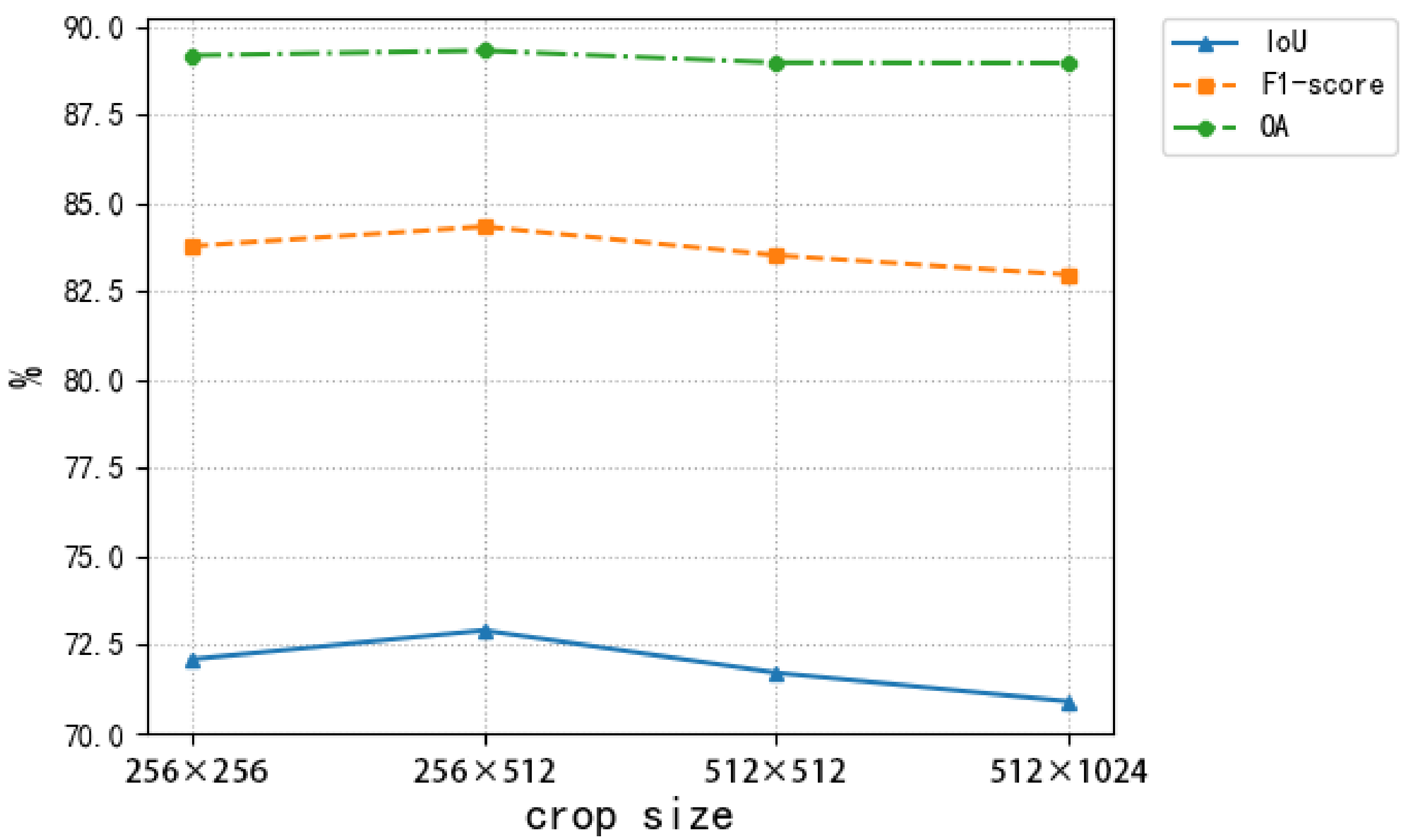
4.4. Sensitivity Analysis on Input Image Size

The geometry of the urban community green space is irregular in high-resolution photos, and the texture is smooth. As a result, a sufficient training sample size can preserve the shape and textural features of distinct objects, enhancing classification accuracy. We evaluated four alternative crop sizes on our approach to see how they affected the output image size: $256\times 256$, $256\times 512$, $512\times 512$, and $512\times 1024$. Figure 10 shows the categorization accuracy obtained with various crop sizes. It was discovered that a crop size of $256\times 512$ produced the greatest results.

5. Conclusions

Urban Community Green Space (UCGS) is a vital component of the city. Methods that can accurately identify urban community green space can provide data for studies that focus on urban design and resident health, which need to break through the scale limitations and shadow interference of current studies. In this research, we created a neighborhood-scale urban community green space (UCGS) dataset and proposed a segmentation decoder with two auxiliary branches for HRNet. The proposed model has shown the most accurate UCGS detection accuracy among all comparison models, with a precision of 83.01, recall of 85.69, IoU of 72.91, F1-score of 84.33, and OA of 89.31. In particular, it achieved a great improvement in the identification of green spaces covered by shadows. Additionally, our discussion demonstrated that the best performance was achieved by two auxiliary decoders (one had $f_2$, $f_3$, $f_4$ as input and the other had $f_3$, $f_4$ as input) with equal weight of 0.4, and OHEM and random rescale techniques can boost the performance. The case results of Shanghai show that the coverage of UCGS in four typical areas is 19%, 12.14%, 22.32%, and 21.62%, respectively.

In future studies, researchers can also focus on community-scale green space identification and exploit simpler and more effective methods to obtain accurate UCGS extraction maps. Our study can provide a trained model for other scholars to perform transfer learning when studying similar problems.

References

1. Kabisch, N.; Haase, D. Green spaces of European cities revisited for 1990–2006. Landsc. Urban Plan. 2013, 110, 113–122. [Google Scholar] [CrossRef]
2. Xu, X.; Duan, X.; Sun, H.; Sun, Q. Green Space Changes and Planning in the Capital Region of China. Environ. Manag. 2011, 47, 456–467. [Google Scholar] [CrossRef] [PubMed]
3. Kopecká, M.; Szatmári, D.; Rosina, K. Analysis of Urban Green Spaces Based on Sentinel-2A: Case Studies from Slovakia. Land 2017, 6, 25. [Google Scholar] [CrossRef] [Green Version]
4. Xu, X.; Li, L.; Shen, J.; Sun, Y.; Lian, Z. Five hypotheses concerned with bedroom environment and sleep quality: A questionnaire survey in Shanghai city, China. Build. Environ. 2021, 205, 108252. [Google Scholar] [CrossRef]
5. Cao, T.; Lian, Z.; Zhu, J.; Xu, X.; Du, H.; Zhao, Q. Parametric study on the sleep thermal environment. Build. Simul. 2021, 15, 885–898. [Google Scholar] [CrossRef]
6. Xu, X.; Lian, Z.; Shen, J.; Lan, L.; Sun, Y. Environmental factors affecting sleep quality in summer: A field study in Shanghai, China. J. Therm. Biol. 2021, 99, 102977. [Google Scholar] [CrossRef]
7. Gupta, K.; Kumar, P.; Pathan, S.; Sharma, K. Urban Neighborhood Green Index—A measure of green spaces in urban areas. Landsc. Urban Plan. 2012, 105, 325–335. [Google Scholar] [CrossRef]
8. Han, J.; Zhao, X.; Zhang, H.; Liu, Y. Analyzing the Spatial Heterogeneity of the Built Environment and Its Impact on the Urban Thermal Environment—Case Study of Downtown Shanghai. Sustainability 2021, 13, 11302. [Google Scholar] [CrossRef]
9. Huerta, R.E.; Yépez, F.D.; Lozano-García, D.F.; Guerra Cobián, V.H.; Ferriño Fierro, A.L.; de León Gómez, H.; Cavazos González, R.A.; Vargas-Martínez, A. Mapping Urban Green Spaces at the Metropolitan Level Using Very High Resolution Satellite Imagery and Deep Learning Techniques for Semantic Segmentation. Remote Sens. 2021, 13, 2031. [Google Scholar] [CrossRef]
10. Shojanoori, R.; Shafri, H. Review on the use of remote sensing for urban forest monitoring. Arboric. Urban For. 2016, 42, 400–417. [Google Scholar] [CrossRef]
11. Wang, G. Concatenated Residual Attention UNet for Semantic Segmentation of Urban Green Space. Forests 2021, 12, 1441. [Google Scholar]
12. Lanlan, W.; Lirong, X.; Hui, P. Quantitative evaluation of field oilseed rape image segmentation based on RGB vegetation index. J. Huazhong Agric. Univ. 2019, 38, 5. [Google Scholar]
13. Tucker, C.J.; Pinzon, J.E.; Brown, M.E.; Slayback, D.A.; Pak, E.W.; Mahoney, R.; Vermote, E.F.; Saleous, N.E. An extended AVHRR 8-km NDVI dataset compatible with MODIS and SPOT vegetation NDVI data. Int. J. Remote Sens. 2005, 26, 4485–4498. [Google Scholar] [CrossRef]
14. Khan, B.; Yang, S.; Hong, W.; Yan, H. Extraction of Urban Green Spaces Based on Gaofen-2 Satellite Imagery. IOP Conf. Ser. Earth Environ. Sci. 2021, 693, 012119. [Google Scholar] [CrossRef]
15. Huete, A.R. A soil-adjusted vegetation index (SAVI). Remote Sens. Environ. 1988, 25, 295–309. [Google Scholar] [CrossRef]
16. Huete, A.; Didan, K.; Miura, T.; Rodriguez, E.P.; Gao, X.; Ferreira, L.G. Overview of the radiometric and biophysical performance of the MODIS vegetation indices. Remote Sens. Environ. 2002, 83, 195–213. [Google Scholar] [CrossRef]
17. Ostu, N. A threshold selection method from gray-histogram. IEEE Trans. Syst. Man Cybern. 1979, 9, 62–66. [Google Scholar]
18. Shen, C.; Li, M.; Li, F.; Chen, J.; Lu, Y. Study on urban green space extraction from QUICKBIRD imagery based on decision tree. In Proceedings of the 18th International Conference on Geoinformatics: GIScience in Change, Geoinformatics 2010, Beijing, China, 18–20 June 2010; pp. 1–4. [Google Scholar] [CrossRef]
19. Kluczek, M.; Zagajewski, B.; Kycko, M. Airborne HySpex Hyperspectral Versus Multitemporal Sentinel-2 Images for Mountain Plant Communities Mapping. Remote Sens. 2022, 14, 1209. [Google Scholar] [CrossRef]
20. Maxwell, A.E.; Warner, T.A.; Fang, F. Implementation of machine-learning classification in remote sensing: An applied review. Int. J. Remote Sens. 2018, 39, 2784–2817. [Google Scholar] [CrossRef] [Green Version]
21. Feng, Q.; Liu, J.; Gong, J. UAV Remote Sensing for Urban Vegetation Mapping Using Random Forest and Texture Analysis. Remote Sens. 2015, 7, 1074–1094. [Google Scholar] [CrossRef] [Green Version]
22. Dempster, A.P. Maximum likelihood from incomplete data via the EM algorithm. J. R. Stat. Soc. 1977, 39, 1–22. [Google Scholar]
23. Blakey, T.; Melesse, A.; Hall, M.O. Supervised Classification of Benthic Reflectance in Shallow Subtropical Waters Using a Generalized Pixel-Based Classifier across a Time Series. Remote Sens. 2015, 7, 5098–5116. [Google Scholar] [CrossRef] [Green Version]
24. Mengya, L.I.; Zhu, X.; Jia, X. Urban Green Space Extraction Based on Object Oriented High Resolution Remote Sensing Data. Beijing Surv. Mapp. 2019, 2, 196–200. [Google Scholar]
25. Fung, T.; So, L.L.H.; Chen, Y.; Shi, P.; Wang, J. Analysis of green space in Chongqing and Nanjing, cities of China with ASTER images using object-oriented image classification and landscape metric analysis. Int. J. Remote Sens. 2008, 29, 7159–7180. [Google Scholar] [CrossRef]
26. Whiteside, T.G.; Boggs, G.S.; Maier, S.W. Comparing object-based and pixel-based classifications for mapping savannas. Int. J. Appl. Earth Obs. Geoinf. 2011, 13, 884–893. [Google Scholar] [CrossRef]
27. Mäyrä, J.; Keski-Saari, S.; Kivinen, S.; Tanhuanpää, T.; Hurskainen, P.; Kullberg, P.; Poikolainen, L.; Viinikka, A.; Tuominen, S.; Kumpula, T.; et al. Tree species classification from airborne hyperspectral and LiDAR data using 3D convolutional neural networks. Remote Sens. Environ. 2021, 256, 112322. [Google Scholar] [CrossRef]
28. Gidaris, S.; Komodakis, N. Object Detection via a Multi-region and Semantic Segmentation-Aware CNN Model. In Proceedings of the IEEE International Conference on Computer Vision (ICCV), Washington, DC, USA, 7–13 December 2015. [Google Scholar]
29. Xu, Z.; Zhou, Y.; Wang, S.; Wang, L.; Wang, Z. U-Net for urban green space classification in GF-2 remote sensing images. Image Graph 2021, 26, 14. [Google Scholar]
30. Shelhamer, E.; Long, J.; Darrell, T. Fully convolutional networks for semantic segmentation. IEEE Trans. Pattern Anal. Mach. Intell. 2017, 39, 640–651. [Google Scholar] [CrossRef]
31. Ronneberger, O.; Fischer, P.; Brox, T. U-net: Convolutional networks for biomedical image segmentation. In Proceedings of the International Conference on Medical Image Computing and Computer-Assisted Intervention, Munich, Germany, 5–9 October 2015; Springer: Cham, Switzerland, 2015; pp. 234–241. [Google Scholar]
32. Zhao, H.; Shi, J.; Qi, X.; Wang, X.; Jia, J. Pyramid Scene Parsing Network. In Proceedings of the IEEE Conference on Computer Vision and Pattern Recognition (CVPR), Honolulu, HI, USA, 21–26 July 2017. [Google Scholar]
33. Chen, L.C.; Zhu, Y.; Papandreou, G.; Schroff, F.; Adam, H. Encoder-Decoder with Atrous Separable Convolution for Semantic Image Segmentation. In Proceedings of the European Conference on Computer Vision ECCV, Munich, Germany, 8–14 September 2018. [Google Scholar]
34. Liu, W.; Yue, A.; Shi, W.; Ji, J.; Deng, R. An Automatic Extraction Architecture of Urban Green Space Based on DeepLabv3plus Semantic Segmentation Model. In Proceedings of the 2019 IEEE 4th International Conference on Image, Vision and Computing (ICIVC), Xiamen, China, 5–7 July 2019. [Google Scholar]
35. Zhou, C.; Xianyun, F.; Xiangwei, G.; Xiaoxue, W.; Huimin, Z. Extraction of urban green space with high resolution remote sensing image segmentation. Bull. Surv. Mapp. 2020, 12, 17–20. [Google Scholar]
36. Xu, Z.; Zhou, Y.; Wang, S.; Wang, L.; Wang, Z. A Novel Intelligent Classification Method for Urban Green Space Based on High-Resolution Remote Sensing Images. Remote Sens. 2020, 12, 3845. [Google Scholar] [CrossRef]
37. Nijhawan, R.; Sharma, H.; Sahni, H.; Batra, A. A Deep Learning Hybrid CNN Framework Approach for Vegetation Cover Mapping Using Deep Features. In Proceedings of the International Conference on Signal-image Technology & Internet-Based Systems, SITIS 2017, Jaipur, India, 4–7 December 2017. [Google Scholar]
38. Jin, B.; Ye, P.; Zhang, X.; Song, W.; Li, S. Object-Oriented Method Combined with Deep Convolutional Neural Networks for Land-Use-Type Classification of Remote Sensing Images. J. Indian Soc. Remote Sens. 2019, 47, 951–965. [Google Scholar] [CrossRef] [Green Version]
39. Fan, Y.; Ding, X.; Wu, J.; Ge, J.; Li, Y. High spatial-resolution classification of urban surfaces using a deep learning method. Build. Environ. 2021, 200, 107949. [Google Scholar] [CrossRef]
40. Tong, X.Y.; Xia, G.S.; Lu, Q.; Shen, H.; Li, S.; You, S.; Zhang, L. Land-cover classification with high-resolution remote sensing images using transferable deep models. Remote Sens. Environ. 2020, 237, 111322. [Google Scholar] [CrossRef] [Green Version]
41. ISPRS Potsdam. Available online: http://www2.isprs.org/commissions/comm3/wg4/2d-sem-label-potsdam.html (accessed on 28 April 2022).
42. ISPRS Vaihingen. Available online: http://www2.isprs.org/commissions/comm3/wg4/2d-sem-label-vaihingen.html (accessed on 28 April 2022).
43. Wang, J.; Zheng, Z.; Ma, A.; Lu, X.; Zhong, Y. LoveDA: A Remote Sensing Land-Cover Dataset for Domain Adaptive Semantic Segmentation. In Proceedings of the Neural Information Processing Systems Track on Datasets and Benchmarks 1, NeurIPS Datasets and Benchmarks 2021, Virtual, 6 December 2021. [Google Scholar]
44. Yang, Z.; Fang, C.; Li, G.; Mu, X. Integrating multiple semantics data to assess the dynamic change of urban green space in Beijing, China. Int. J. Appl. Earth Obs. Geoinf. 2021, 103, 102479. [Google Scholar] [CrossRef]
45. Moreno-Armendáriz, M.A.; Calvo, H.; Duchanoy, C.A.; López-Juárez, A.P.; Vargas-Monroy, I.A.; Suárez-Castañón, M.S. Deep Green Diagnostics: Urban Green Space Analysis Using Deep Learning and Drone Images. Sensors 2019, 19, 5287. [Google Scholar] [CrossRef] [Green Version]
46. Wang, L.; Zhang, C.; Li, R.; Duan, C.; Meng, X.; Atkinson, P.M. Scale-Aware Neural Network for Semantic Segmentation of Multi-Resolution Remote Sensing Images. Remote Sens. 2021, 13, 5015. [Google Scholar] [CrossRef]
47. Gong, Y.; Li, X.; Cong, X.; Liu, H. Research on the Complexity of Forms and Structures of Urban Green Spaces Based on Fractal Models. Complexity 2020, 2020, 4213412. [Google Scholar] [CrossRef]
48. Tu, Q. Shanghai Master Plan 2017–2035: “Excellent Global City”. Tous Urbains 2019, 27–28, 58–63. [Google Scholar]
49. Wu, Z.; Chen, R.; Meadows, M.E.; Sengupta, D.; Xu, D. Changing urban green spaces in Shanghai: Trends, drivers and policy implications. Land Use Policy 2019, 87, 104080. [Google Scholar] [CrossRef]
50. SMSB. Shanghai Urban Green Space In Main Years. Available online: http://tjj.sh.gov.cn/tjnj/nj20.htm?d1=2020tjnjen/E1116.htm (accessed on 30 April 2022).
51. Sky Map. Available online: http://shanghai.tianditu.gov.cn/map/views/map.html (accessed on 30 April 2022).
52. 91 Satellite Image Assistant. Available online: http://www.qianfansoft.net/ (accessed on 30 April 2022).
53. National Platform for Common Geospatial Information Services. Available online: https://www.tianditu.gov.cn/ (accessed on 30 April 2022).
54. Shanghai Surveying & Mapping Institute. Available online: http://www.shsmi.cn/ (accessed on 30 April 2022).
55. Nan, K.K.; Zhi-Gang, L.I.; Xie, C.K.; Che, S.Q. Effect of Green Space Structure on the Thermal Environment of Residential Area in Shanghai. J. Shanghai Jiaotong Univ. Agric. Sci. 2016, 34, 61–67. [Google Scholar]
56. Feng, Y.; Yang, Q.; Hong, Z.; Cui, L. Modelling coastal land use change by incorporating spatial autocorrelation into cellular automata models. Geocarto Int. 2018, 33, 470–488. [Google Scholar] [CrossRef]
57. Chen, D.; Long, X.; Li, Z.; Liao, C.; Xie, C.; Che, S. Exploring the Determinants of Urban Green Space Utilization Based on Microblog Check-In Data in Shanghai, China. Forests 2021, 12, 1783. [Google Scholar] [CrossRef]
58. Labelme Tool. Available online: http://labelme2.csail.mit.edu/Release3.0/ (accessed on 30 April 2022).
59. Ministry of Construction. National Garden and Park Urban Standard; Number 106; Urban Construction: Seoul, Korea, 2000. [Google Scholar]
60. Gao, X.; Zhang, Z.; Fei, X. Urban Green Space Landscape Pattern Evaluation Based on High Spatial Resolution Images. In Proceedings of the Geo-Informatics in Resource Management and Sustainable Ecosystem—International Symposium, GRMSE 2013, Wuhan, China, 8–10 November 2013; Proceedings, Part I, Communications in Computer and Information Science. Bian, F., Xie, Y., Cui, X., Zeng, Y., Eds.; Springer: Berlin/Heidelberg, Germany, 2013; Volume 398, pp. 100–106. [Google Scholar] [CrossRef]
61. Weng, X.; Yan, Y.; Dong, G.; Shu, C.; Wang, B.; Wang, H.; Zhang, J. Deep Multi-Branch Aggregation Network for Real-Time Semantic Segmentation in Street Scenes. arXiv 2022, arXiv:2203.04037. [Google Scholar] [CrossRef]
62. Ernst, P.; Ghosh, S.; Rose, G.; Nürnberger, A. Dual Branch Prior-SegNet: CNN for Interventional CBCT using Planning Scan and Auxiliary Segmentation Loss. arXiv 2022, arXiv:2205.10353. [Google Scholar]
63. Toshniwal, S.; Tang, H.; Lu, L.; Livescu, K. Multitask Learning with Low-Level Auxiliary Tasks for Encoder-Decoder Based Speech Recognition. arXiv 2017, arXiv:1704.01631. [Google Scholar]
64. Russo, P.; Tommasi, T.; Caputo, B. Towards Multi-source Adaptive Semantic Segmentation. In Proceedings of the Image Analysis and Processing—ICIAP 2019—20th International Conference, Trento, Italy, 9–13 September 2019; Proceedings, Part I, Lecture Notes in Computer Science. Ricci, E., Bulò, S.R., Snoek, C., Lanz, O., Messelodi, S., Sebe, N., Eds.; Springer: Berlin/Heidelberg, Germany, 2019; Volume 11751, pp. 292–301. [Google Scholar] [CrossRef]
65. Zhang, X.; Zhu, X.; Zhang, X.; Zhang, N.; Li, P.; Wang, L. SegGAN: Semantic Segmentation with Generative Adversarial Network. In Proceedings of the Fourth IEEE International Conference on Multimedia Big Data, BigMM 2018, Xi’an, China, 13–16 September 2018; pp. 1–5. [Google Scholar] [CrossRef]
66. Sun, K.; Xiao, B.; Liu, D.; Wang, J. Deep High-Resolution Representation Learning for Human Pose Estimation. arXiv 2019, arXiv:1902.09212. [Google Scholar]
67. Yu, C.; Gao, C.; Wang, J.; Yu, G.; Shen, C.; Sang, N. BiSeNet V2: Bilateral Network with Guided Aggregation for Real-Time Semantic Segmentation. Int. J. Comput. Vis. 2021, 129, 3051–3068. [Google Scholar] [CrossRef]
68. Liu, S.; Davison, A.J.; Johns, E. Self-supervised generalisation with meta auxiliary learning. In Proceedings of the 33rd International Conference on Neural Information Processing Systems 2019, NeurIPS 2019, Vancouver, BC, Canada, 4–8 December 2019; pp. 1679–1689. [Google Scholar]
69. Radford, A.; Narasimhan, K. Improving Language Understanding by Generative Pre-Training. OpenAI Blog 2018. in progress. [Google Scholar]
70. Shrivastava, A.; Gupta, A.; Girshick, R. Training Region-based Object Detectors with Online Hard Example Mining. In Proceedings of the Conference on Computer Vision and Pattern Recognition (CVPR), Las Vegas, NV, USA, 27–30 July 2016. [Google Scholar]
71. Huang, Q.; Sun, J.; Hui, D.; Wang, X.; Wang, G. Robust liver vessel extraction using 3D U-Net with variant dice loss function. Comput. Biol. Med. 2018, 101, S0010482518302385. [Google Scholar] [CrossRef]
72. White, A.E.; Dikow, R.B.; Baugh, M.; Jenkins, A.; Frandsen, P.B. Generating segmentation masks of herbarium specimens and a data set for training segmentation models using deep learning. Appl. Plant Sci. 2020, 8, e11352. [Google Scholar] [CrossRef]
73. Liu, H.; Feng, J.; Feng, Z.; Lu, J.; Zhou, J. Left Atrium Segmentation in CT Volumes with Fully Convolutional Networks. In Proceedings of the Deep Learning in Medical Image Analysis and Multimodal Learning for Clinical Decision Support—Third International Workshop, DLMIA 2017, and 7th International Workshop, ML-CDS 2017, Held in Conjunction with MICCAI 2017, Québec City, QC, Canada, 14 September 2017; Lecture Notes in Computer Science. Cardoso, M.J., Arbel, T., Carneiro, G., Syeda-Mahmood, T.F., Tavares, J.M.R.S., Moradi, M., Bradley, A.P., Greenspan, H., Papa, J.P., Madabhushi, A., et al., Eds.; Springer: Cham, Switerland, 2017; Volume 10553, pp. 39–46. [Google Scholar] [CrossRef]
74. Dice, L.R. Measures of the Amount of Ecologic Association Between Species. Ecology 1944, 26, 297–302. [Google Scholar] [CrossRef]
75. Guindon, B.; Zhang, Y. Application of the Dice Coefficient to Accuracy Assessment of Object-Based Image Classification. Can. J. Remote Sens. 2017, 43, 48–61. [Google Scholar] [CrossRef]
76. QGIS. Available online: https://www.qgis.org/en/site/ (accessed on 6 June 2022).
77. Fleet, C.; Kowal, K.C.; Pridal, P. Georeferencer: Crowdsourced Georeferencing for Map Library Collections. D-Lib Mag. 2012, 18, 52. [Google Scholar] [CrossRef]
78. Contributors, M. MMSegmentation: OpenMMLab Semantic Segmentation Toolbox and Benchmark. 2020. Available online: https://github.com/open-mmlab/mmsegmentation (accessed on 6 June 2022).
79. Wong, S.C.; Gatt, A.; Stamatescu, V.; McDonnell, M.D. Understanding Data Augmentation for Classification: When to Warp? In Proceedings of the 2016 International Conference on Digital Image Computing: Techniques and Applications (DICTA) 2016, Gold Coast, Australia, 30 November–2 December 2016; pp. 1–6. [Google Scholar] [CrossRef] [Green Version]
80. Zheng, Q.; Yang, M.; Tian, X.; Jiang, N.; Wang, D. A Full Stage Data Augmentation Method in Deep Convolutional Neural Network for Natural Image Classification. Discret. Dyn. Nat. Soc. 2020, 2020, 11. [Google Scholar] [CrossRef]
81. Chen, L.; Papandreou, G.; Schroff, F.; Adam, H. Rethinking Atrous Convolution for Semantic Image Segmentation. arXiv 2017, arXiv:1706.05587. [Google Scholar]
82. He, K.; Zhang, X.; Ren, S.; Sun, J. Deep Residual Learning for Image Recognition. In Proceedings of the IEEE Conference on Computer Vision and Pattern Recognition (CVPR), Las Vegas, NV, USA, 27–30 June 2016. [Google Scholar]
83. Deng, J.; Dong, W.; Socher, R.; Li, L.J.; Li, K.; Dept, F.F. ImageNet: A Large-Scale Hierarchical Image Database. In Proceedings of the 2009 IEEE Conference on Computer Vision and Pattern Recognition, Miami, FL, USA, 20–25 June 2009. [Google Scholar]
84. He, T.; Zhang, Z.; Zhang, H.; Zhang, Z.; Xie, J.; Li, M. Bag of Tricks for Image Classification with Convolutional Neural Networks. In Proceedings of the IEEE Conference on Computer Vision and Pattern Recognition, CVPR 2019, Long Beach, CA, USA, 16–20 June 2019; pp. 558–567. [Google Scholar] [CrossRef] [Green Version]
85. Stefanidis, S.P.; Chatzichristaki, C.A.; Stefanidis, P.S. An ArcGIS toolbox for estimation and mapping soil erosion. J. Environ. Prot. Ecol. 2021, 22, 689–696. [Google Scholar]
86. Ruder, S. An Overview of Multi-Task Learning in Deep Neural Networks. arXiv 2017, arXiv:1706.05098. [Google Scholar]
87. Garcia-Garcia, A.; Orts-Escolano, S.; Oprea, S.; Villena-Martinez, V.; Rodríguez, J.G. A Review on Deep Learning Techniques Applied to Semantic Segmentation. arXiv 2017, arXiv:1704.06857. [Google Scholar]
Figure 1. Proposed Workflow for UCGS extraction.
Land 11 00905 g001
Figure 2. Study Area. (A) is located in Baoshan District. (B) is located on the Bund, straddling Huangpu District and Pudong New Area. (C) is located in the new city of Pudong New Area. (D) is located in the suburban Minhang District.
Land 11 00905 g002
Figure 3. Different types of residential green space in the dataset.
Land 11 00905 g003
Figure 4. Illustration of the proposed auxiliary learning for HRNet (aux-HRNet) model, which is improved from HRNetV2. Different combinations of low-resolution feature maps are sent into two auxiliary decoders. The color of the feature map decreases in resolution by yellow, orange, pink and red. The major loss and auxiliary loss are denoted by the terms “Main Loss” and “Aux Loss”, respectively.
Land 11 00905 g004
Figure 5. Decoders and auxiliary decoders for HRNet. (a) HRNetV2. (b) auxiliary decoder with three low-resolution subnets as input. (c) auxiliary decoder with two low-resolution subnets as input.
Land 11 00905 g005
Figure 6. Segmentation results of different types of green spaces. (a) residential area separation zone. (b) small public green space. (c) green space along the street. (d) scattered trees. White means UCGS while black means other, respectively.
Land 11 00905 g006
Figure 7. Comparison of shaded green space recognition performance between HRNet and our model. (a) is selected from a image with brighter shadow. (b) is selected from the one with dark shadow. The red box circled is the shadow area cast by the tall building, and the white part inside the box is actually the green space.
Land 11 00905 g007
Figure 8. Predicted results: the mapping results of urban community green space in four selected areas in Shanghai with different percentage of UCGS. Here subplots (AD) correspond to subplots (A–D) of Figure 2.
Land 11 00905 g008
Figure 9. Different weights of auxiliary loss. (a) fix β = 0.4 and change α . (b) fix α = 0.4 and change β . (c) fix β = α and change both. Baseline means the result of HRNetV2.
Land 11 00905 g009
Figure 10. UCGS extraction accuracy varies with different crop sizes.
Land 11 00905 g010