Article

Land Use Changes for Investments in Silvoarable Agriculture Projected by the CLUE-S Spatio-Temporal Model

by
Stamatia Nasiakou
1,
Michael Vrahnakis
2,*,
Dimitrios Chouvardas
3,
Georgios Mamanis
1 and
Vassiliki Kleftoyanni
1
1
University of Thessaly, GR-38221 Volos, Greece
2
Department of Forestry, Wood Sciences and Design, University of Thessaly, GR-43131 Karditsa, Greece
3
Department of Forestry and Natural Environment, Aristotle University, GR-54124 Thessaloniki, Greece
*
Author to whom correspondence should be addressed.
Land 2022, 11(5), 598; https://doi.org/10.3390/land11050598
Submission received: 10 March 2022 / Revised: 12 April 2022 / Accepted: 17 April 2022 / Published: 19 April 2022

Abstract

:
Investment in biology-based technological innovations is a key requirement for the development of modern agriculture/forestry. The expansion of innovative biological technologies includes changes in crops/cultivations, such as the transition from intensive monocultures to multiple crops of lower agrochemical inputs with the integration of woody trees/shrubs or animals, represented by Agroforestry. This innovative biological technology is further promoted at the European Union (EU) level by powerful institutions such as the Green Deal and the new CAP, mainly by tools such as ecoschemes and agri-environmental and climate measures (AECMs). The use of integrated regional spatiotemporal models, such as CLUE-S, to predict land use changes in the framework of Agroforestry is rather restricted. This paper examines Agroforestry as a vehicle that can contribute to achieving the rural development of the region of Thessaly, Greece. It sets a time horizon for reviewing the changes that are expected in the most important units of land uses of the rural landscape of the municipality of Mouzaki, western Thessaly plain, in the year 2040, which serves as model land for the region of Thessaly. It examines these changes with the effect of three (3) socio-economic scenarios: (a) a linear operating scenario (business as usual, BAU), (b) an ecological land protection (ELP) scenario, and (c) a rapid economic development (RED) scenario. These scenarios were introduced in the non-spatial module of the CLUE-S spatiotemporal model, while in the spatial module sixteen (16) characteristic landscape parameters were introduced as independent variables. The most important land use units, including traditional silvoarable and silvopastoral woodland systems, were the dependent variables. The simulations of the changes of the land use units showed that under the RED scenario, in the year 2040 the extent of the silvoarable systems is expected to increase significantly (57%) compared to the reference year of 2020, while the rest of the land use units under the other scenarios are mainly regulated by depopulation/abandonment of the rural areas and the processes of natural succession. The fact that the extent of silvoarable systems is increasing, in combination with the favorable institutional environment created by European rural policies, gives impetus to regional rural development through investments in the agricultural sector and mainly in Agroforestry systems.

1. Introduction

The modern concept of multidimensional rural development requires innovative tools that will fulfill its multiple purposes. In contrast to the one-dimensional economic view of rural innovation described by Schultz’s [1] high-pay-off model, Hayami and Ruttan’s [2] model of technical change seems to fit in better with modern requirements. Such an economic view of agriculture, and especially the form of post-production operation of the model of technical change, has been widely accepted by modern theorists (e.g., Jin and Jorgenson [3]). The term technical change does not only mean technological innovations (such as new agricultural machinery), but also biological ones. Thus, investment in biology-based technological innovations is a key requirement for rural development. The expansion of innovative biological technologies includes the change of crops, such as the transition from intensive monocultures to multiple crops of lower inputs with the integration of woody trees/shrubs or animals, represented by Agroforestry.
The primary productive activity of the combination of agricultural crops of trees and/or grazing farm animals in the same unit of land area is called Agroforestry, and the part of the land that is very susceptible to such activity is called an Agroforestry system. Agroforestry has a high potential to be a viable alternative to crop change (Nasiakou [4]). Benefits of the transition from monoculture to an Agroforestry system have been observed in many developed countries with robust economies. Agroforestry is a sustainable practice, compatible with the main goal of overall sustainable development for Australia (George et al. [5]) or Canada (De Baets et al. [6]). However, Agroforestry is a much more important lever for economic upgrading for those countries that have experienced some kind of economic recession/slowdown and are in economic recovery. Such reports come from Rwanda (Stainback et al. [7]), the Philippines (Neyra-Cabatac et al. [8]), Bangladesh (Islam et al. [9]), or China under reform (Ren et al. [10]). Likewise, for Greece, Agroforestry is projected as a prospect of economic recovery after the economic crisis of recent years (Nasiakou and Vrahnakis [11]).
Streed [12] distinguishes the economic benefits for the owner of an agroforestry farm, in the form of additional land income. These revenues may include marketable timber, non-timber forest products (such as food, medicine, or resin), crop and pasture crop yields, and inflows or grants from government programs such as the US Conservation Reserve, US Programs, or state Rural Development Programs, specializing in the European Union’s (EU) Common Agricultural Policy (CAP). In line with such considerations as Streed’s [12], the global recognition of the profitability of agroforestry systems is clearly reflected in the World Bank’s Agriculture Investment Sourcebook (World Bank [13]). Specifically, Agroforestry is included in Section 5 entitled Investments in Sustainable Natural Resource Management for Agriculture (Module 5—Investments in Sustainable Natural Resource Management for Agriculture).
From the above, it is evident that land use change towards Agroforestry is a promising lever for investment in the primary sector. This is especially important for intensively used rural landscapes with extensive domination of monocultures. By using, as a physical model, the area of municipality of Mouzaki, which is representative of the intensively cultivated plain of Thessaly in central Greece, the purpose of this paper is to indicate the most suitable socioeconomic scenario for investing in Agroforestry. These scenarios have already built and presented by Mamanis et al. [14]. Land use changes that are anticipated to emerge within a time frame of 20 years (2020–2040) are produced by the projections of the CLUE-S spatiotemporal model (Veldkamp and Fresco [15,16]). The institutional environment needed to invest in Agroforestry in the region of Thessaly, and elsewhere in the EU, is further discussed.

2. The CLUE-S Spatiotemporal Model

There have been several reviews of efforts to integrate modeling of economy-environment-society interactions, as well as the consequences of these factors on land use. Most have concluded that the number of models in which land use change is adequately modeled is very small (Turner et al. [17], Fischer et al. [18], Lonergan and Prudham [19]). One possible explanation is that the original purpose of most was not to model land use change, per se (Briassulis [20]). The IIASA’s LUC (Fischer et al. [18]), IMPEL (Rounsevell [21]), cellular automata (Tobler [22]), and CLUE (Veldkamp and Fresco [15,16]) models are considered to be representative of a more modern type for economy-environment-society interactions. In addition, their immediate purpose is to model land use change. This last feature reflects the recent interest in the critical role of land use change in provoking larger-scale environmental change.
The CLUE (Conversion of Land Use and its Effects) modeling framework was developed, and is still being developed, at the Agricultural University in Wageningen (Netherlands) with the aim of modeling land use changes according to the factors that contribute to them. The original idea for the first version of CLUE was conceived by Tom Veldkamp and Louise Fresco (Veldkamp and Fresco [15,16]), while a first application was presented by the same researchers a year ago (Veldkamp and Fresco [23]). Further impetus to the development of CLUE was given by later editions created by Peter Verburg in collaboration with colleagues at Wageningen University (Verburg et al. [24], de Koning et al. [25]) and as CLUE-S by Verburg et al. [26] and Verburg and Overmars [27]. It has been applied to the analysis of land use/cover changes in many countries, such as the Netherlands (Verburg and Overmars [27]), Malaysia (Verburg et al. [26], Verburg and Overmars [27]), and Ecuador (de Koning et al. [28]), and as DYNA-CLUE by Salazar et al. [29], the Philippines (Verburg et al. [26,30]), Costa Rica (Veldkamp and Fresco [16], Schoorl et al. [31]), Indonesia (Verburg et al. [32]), China (Verburg et al. [33]), and Greece (Chouvardas [34]). The CLUE modeling framework is spatially clear and is used to analyze land use/cover dynamics at various spatial scales. Its latest versions also incorporate dynamic analysis of feedback on land use changes in the local environment, population, etc.; for example, with intensive agricultural land use or inappropriate use in sensitive areas. Thus, the CLUE modeling framework can be described as an integrated, spatially clear, multi-scale, dynamic, economy-environment-society-land use model. It is an interdisciplinary model as it integrates environmental modeling and Geographic Information Systems (Veldkamp and Fresco [16]).
The version of CLUE that has been used most in modeling land use changes, mainly for forecasting purposes, is CLUE-S (Verburg et al. [26], Verburg and Overmars [27]). The CLUE-S model is based on the dynamic simulation of spatial land use change patterns in response to predetermined changes in land demand from different sectors of economic activity (e.g., agriculture and forestry). During each time step, the model determines for each location (grid cell) the appropriate land use, i.e., the specific land use which is determined based on the combination of the suitability of the location itself (for the specific land use) and the competitive advantage that the indicated land use has over others, based on their requirements, i.e., on the basis of demand. If the appropriate land use type for the location requires an unrealistic land use conversion (not allowed due to spatial policies and restrictions) then the next most-appropriate land use type is selected. Spatial policies (such as regional policy), constraints and the matrix of possible conversions must be defined in advance by the user (Verburg and Veldkamp [35]). After allocating the indicated land uses to all locations in the area of interest, the total (cumulative) land use demand is compared to the allocated areas. If demand is not properly distributed, the competitive advantage of the different types of land uses is modified in such a way that the land uses for which the demand was not met have a greater preference. Over-represented land uses have a lower preference. This process is repeated until the demand is met by the assigned area. Demand for different land use types must be determined in advance by the user. The calculation of changes in demand is exogenous in the context of CLUE-S and can be based on different techniques ranging from simple trend extensions to advanced modeling of requirements based on specific socio-economic scenarios.

3. Materials and Methods

3.1. Study Area and Forecasting Period

The research area was the administrative territory of Mouzaki, central Greece (31,326.97 Ha, Figure 1). The municipality includes 27 village communities populated by more than 13,000 inhabitants. Agricultural crops occupied 11,144.03 Ha (35.57%), silvoarable 556.38 Ha (1.78%), grasslands 2405 Ha (7.68%), silvopastoral systems (10–40% tree cover) 3815.39 Ha (12.18%), forests (40–100% tree cover) 10573.64 Ha (33.75%), sparse shrublands (10–40% shrub cover) 503.74 Ha (1.61%), dense shrublands (>40% shrub cover) 784.99 Ha (2.51%), urban 1457.79 Ha (4.65%), and barren land 86.01 Ha (0.27%) (Figure 1, Nasiakou et al. [36]).
A period of twenty years (2020–2040) was chosen as the most appropriate forecast period. This choice is a compromise between the time it takes to see the results of the forecast (the shorter the forecast time, the smaller the change in land use) and the uncertainty that arises if a large time horizon is chosen.

3.2. Variables Input for CLUE-S Model

The CLUE-S model was chosen to be applied in the modeling of land use changes in the landscape of Mouzaki. For the supply of CLUE-S and considering the possibilities of collecting and processing the important landscape driving factors of Mouzaki, sixteen (16) variables were selected (Table 1).

3.3. Selection and Digital Preparation of the Land Uses at Year 2020

The above landscape driving factors were introduced as independent variables in the spatial module of CLUE-S. In addition, land uses were selected as dependent variables. The results of the photo interpretation and digital processing of recent satellite images from the Google Earth Pro program were used to structure the land uses. As with the independent variables, the land use types were converted to (geographically oriented) digital raster files with a pixel size of 100 m. The raster file of each land use was rendered binarily. Thus, each pixel with the presence of the specific land use received the value of 1, and each with its absence the value of 0. The digital raster files were then converted to alphanumeric ascii files to ensure their entry in the statistical program SPSS (ver. 23) as dependent variables of CLUE-S.

3.4. Statistical Analysis

For the logistic regression, the CLUE-S variables were processed using the SPSS. The generated ascii files of the dependent and independent variables were transformed (after the file converter command of CLUE-S) into a table format to be imported into SPSS. The data then were analyzed by the method of binary logistic regression of absence/presence, using Forward: Conditional analysis as a step-by-step regression method. According to Verburg and Veldkamp [35], it is considered the most appropriate logistic regression method for CLUE-S, as it selects those landscape change variables that exhibit the highest degree of correlation, while rejecting those with the lowest degree (Verburg et al. [26]). In the process, the correlation values of the input and output probabilities of the independent variables in the equation should not exceed the significance levels αinput = 0.01 and αoutput = 0.02, respectively (Verburg and Veldkamp [35]). The regression coefficients (bi) of the independent variables that remained in the logistic equation were presented in tabular form. In addition, the following were calculated:
  • The exponential coefficients (EXP (b)), as a result of the increase of the negative logarithm (e) in the value of the coefficients (bi).
  • The Relative Influence Index (RII) of the independent variables, defined as exp(b x variable’s value range).
  • The area under the ROC (Relative Operating Characteristic) curve (AUC) as a measure of controlling the goodness of fit of the data to the logistic regression model.
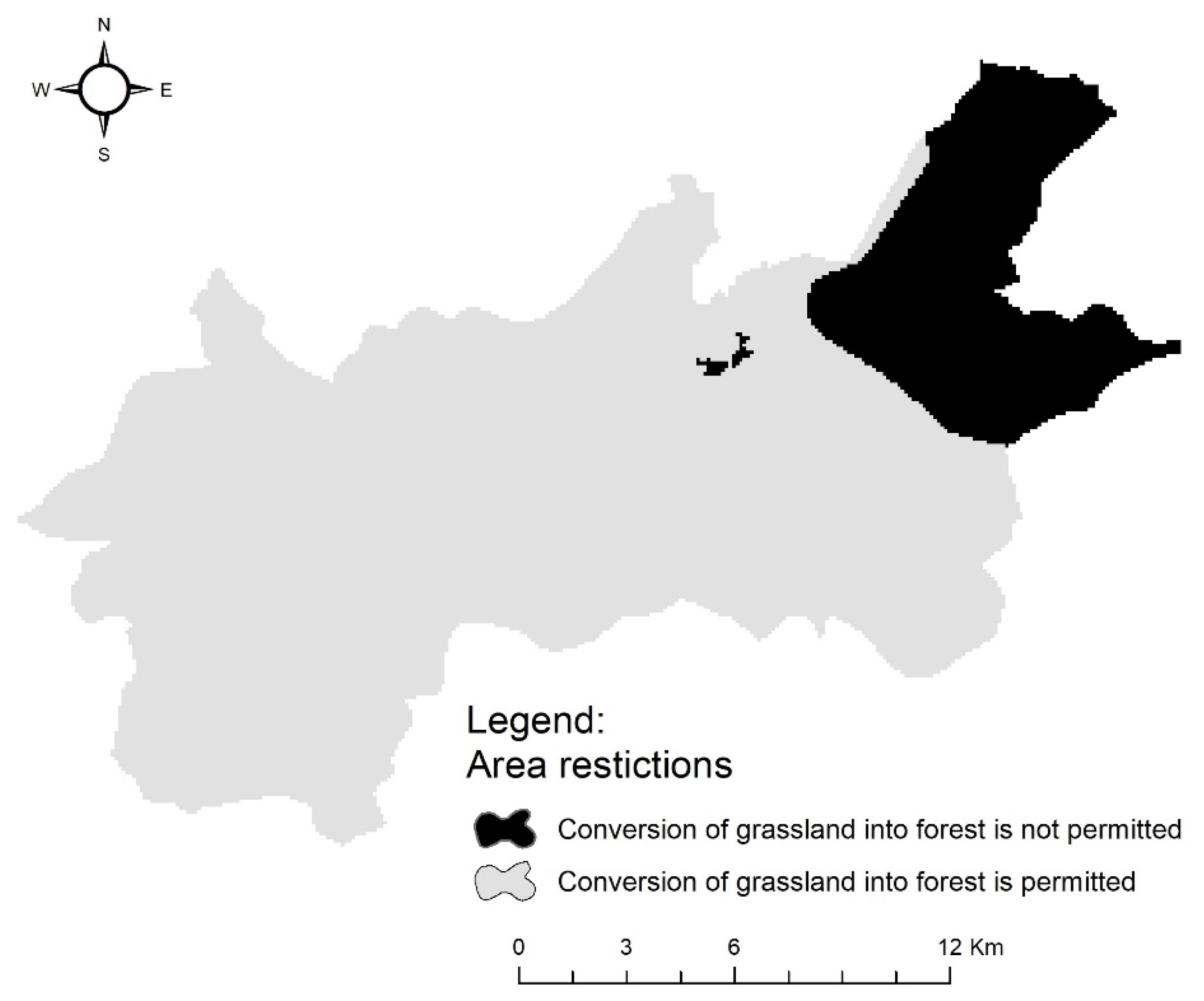
  • The coefficients of elasticity of the land uses of Mouzaki against the drivers of change to which they are exposed. The value of 1 was given to those land uses that are considered stable and unchanged, so the values close to 1, as given to the categories of Unused land, Settlements, and Forests (0.9, Table 2), reflect land uses that show a high degree of stability and are considered difficult to change. The value 0 (or close to 0) was given to land uses that are vulnerable to change, such as Grasslands, Open Shrublands, and Silvopastoral, which are very easily to change. All other land uses received intermediate values (Table 2). Although most transformations were permissible, some, such as those of Dense shrubland and Forests, were considered permissible only in certain land use units. The category of Urban land was considered practically unchanged and a stable unit of the landscape, and for this reason all its transformations to another use took the value of 0. With regard to the constraints that could additionally be defined within the transformation matrix, value 16 stipulated that the conversion of grassland into forest was not permissible in the eastern areas of the landscape (Figure 2). Finally, value 110 stipulated that the direct conversion of grassland into forest would be possible only after a period of at least 10 years.
  • The matrix of permissible transformations of the landscape of Mouzaki, shown in Table 3, where the rows express the current land uses while the columns represent the possible future ones to which the current ones can switch. A value of 1 indicates that transformation is permissible, while a value of 0 indicates that it is not. The results of the diagram of diachronic transformations of the landscape were utilized for the construction of the matrix.

3.5. Socioeconomic Scenarios

In order to predict the land use requirements in the area of Mouzaki, which will be used by CLUE-S, the proposed approach of building scenarios in the context of business research was used (Rosenhaead [37], Weintraub and Bare [38], Wang et al. [39], and Mishra [40]). Scenario analysis is often used to explore future under uncertainties (Liu et al. [41]) Business research manages to effectively enhance environmental decision-making related to multifactorial, social, legal, institutional, technical, and environmental relationships (Mishra [40]). Specifically, the approach of Wang et al. [39] was used, which proposes a model for projecting land use demand based on business research optimization models on ecosystem services for the greater Wuhan city area of China’s Hubei province. The researchers explored how land use change under different scenarios would affect ecosystem service delivery, combining a land use optimization model with an ecosystem service valuation model. The objectives of the research included the forecast of the spatio-temporal dynamics of land use in 2040, using the combined model of Multi-Objective Programming (MOP) and Dyna-CLUE under three different scenarios, i.e., the linear operating scenario or business as usual (BAU), rapid economic development (RED), and ecological land protection (ELP). In the RED scenario the demands were calculated by maximizing the economic benefit of land uses, and in the ELP scenario the demands were calculated by maximizing the environmental benefit of land uses. These three proposed socio-economic scenarios (BAU, RED, and ELP) were adopted by the present study. The twenty year 2020–2040 period was chosen as the most appropriate predicted period for the study. The choice of this period was a compromise between the time it takes to realize the results of the forecast (the shorter the forecast time, the smaller the change in land use) and the uncertainty that would result if a longer time horizon were chosen. Specifically, a scenario model was chosen that uses optimization theory to (a) maximize financial profit and (b) maximize the benefit of ecosystem services. More details about the structure and constraints of the chosen socioeconomic scenarios are found in Mamanis et al. [14].

3.6. Data Processing in CLUE-S

Data processing in CLUE-S included a five-phase process (Verburg [42], Verburg and Veldkamp [35]), with which the future land uses of the landscape of Mouzaki are distributed. In the first phase, the identities of the pixels of the raster file of the landscape of Mouzaki were determined; those that were allowed to change their land use and those which were not allowed, due to restrictions (fixed pixels). In the second phase, the total probability performance of pixels that could be changed in a given land use was calculated, considering the suitability of the pixel position, the coefficient of elasticity of each land use, and the iteration variable of CLUE-S, which gave the relative competitiveness of each land use. In the third phase, an initial distribution of land uses took place, favouring in particular those that presented the largest greater overall probability of response to the demands, while maintaining the same value of the iteration variable for each land use. At this stage there were restrictions on the response of land uses based on the transformation matrix. In the next phase, the model-calculated land use responses per pixel were compared to those of future demand received from the CLUE-S non-spatial module (Figure 3). In cases where, for a land use, the initial response was higher than that of future demand, the recurrence rate decreased, while it correspondingly increased for smaller ones. In this way, the land use recovery was reactivated. Lastly, phases two to four were repeated until the total response of each land use was equal to the values of the future demand of the non-spatial module.

3.7. Production of Probability Maps and Landscape Change

The above five phases were repeated for all forecast time periods. Upon their completion, CLUE-S produced a first group of digital maps of the future change of the landscape of Mouzaki. In addition, CLUE-S enabled the production of a second set of land use probability maps. Probability maps are the expression of the distribution in the landscape of the results of logistic regression equations (Verburg [42]). As the structure of the two map groups was the same as the raster files of the model variables, it was easy to further process them with ArcGIS.

3.8. Model Validation and Calibration

The negative validation (or test of corroboration, Soepboer [43]) of the CLUE-S model was applied. More specifically, this method considers the model to be reliable when it is able to successfully pass a series of critical tests, such as checking the values and range of variables and parameters of the model. First it is ascertained whether the small changes in the variables and the basic parameters of the model bring about corresponding changes in the results of the model and secondly it is ascertained whether the forecast results of the model agree with the logical change of the land use distribution. The model correction process (calibration) was then followed after the application of the above validation test (Englesman et al. [44]) and is the last stage of model validation (Mazzotti and Vinci [45]). The same type of validation and calibration was used during the application of CLUE-S in the landscape of Langadas, northern Greece (Chouvardas [34]). During the process of checking and calibrating the model, it was found that small changes in the variables and parameters of the model brought about the corresponding changes in its results. However, it was then found that the model provided for the conversion of part of the grasslands into forests around the eastern lowland villages, which according to the existing socio-economic conditions is not considered possible and was an unreasonable change in the distribution of land use. In order to correct this, a restriction of conversion of grassland to forests in the eastern lowlands of the landscape was included in the model in the form of a grid file (Figure 1, value 16 of the transformation matrix of Table 3).

4. Results

4.1. Landscape Driving Factors

The digital elevation model of Mouzaki revealed that that over 70% of the landscape belonged to the low zone (0–600 m). About 10% belonged to the middle or semi-mountainous zone (600–800 m), 11% to the mountainous zone (800–1200 m), and the rest (7%) to the pseudo-alpine zone (>1200 m) (Figure 4A). The lowest altitude was 61 m and the highest was 1940 m. The distribution in altitude classes showed that the predominantly low places were located in the central and eastern part of the landscape, while the areas with higher altitude were located west and southwest. The flat and gentle slopes (<15%) prevailed at a rate of approximately 47%, followed by the moderate (15–30%) at a rate of 21%, and the steep and very steep land (>30%) at a rate of 42%. The flat areas (slope < 5%) were located in the eastern part of the landscape, and in streams in the central and eastern part, while the areas with strong and very steep slopes (>30% slope) were located mainly in the mountainous areas west and southwest (Figure 4B). The parent rock consisted of the largest percentage of very deep alluvial deposits in the eastern center-north, with a percentage of 41% approximately, and the deep on-schist soils occupied about 26% of the total area and were located in the western, southern, and central-southern part of Mouzaki. The limestone was located in moderately deep, shallow to rocky soils that occupied about 23% of the total area and dominated the central Mouzaki, while elongated lime formations appeared in the western part between schist (Figure 4C). The soils appeared slightly eroded (0–12 t/Ha/year), mainly in the eastern part where gentle slopes and alluvial deep soils prevailed (Figure 4D). The erosion potential became more intense in the central and western part as the slopes increased, mainly on schist and limestone, while in the mountainous areas it became very high and could reach 190 t/Ha/year. Given the intense agricultural activity, the road network was particularly dense in the western plain part (Figure 4E). Respectively, the existence of many settlements in the rest of Mouzaki was associated with dense road networks in these areas. Places with a distance of more than 1500 m from a road network were located sporadically in the mountainous part. The hydrological network was diverse, as most of was formed by a multitude of streams and rivers, but not of permanent flow (Figure 4F). Locations with relatively long distances were found in the western part of the mountains and in a spot in the northeast. The landscape was characterized by 32 urban centers (Figure 4G). Consequently, the distances in relation to the urban centers were short and not more than 5100 m. In general, the longest distances were located in the periphery of the municipality, mainly in the south-western part. The distribution of the population size of the permanent residents per unit area of Mouzaki indicated that the class with the highest relative population density (0.8–2.0 inhabitants/Ha) was located in the urban centers of Mouzaki and Mavromati (Figure 4H). However, seven (7) urban centers had a very low population density (<0.2 inhabitants/Ha) and eight (8) centers had low density (0.21–0.35 inhabitants/Ha). Regarding the distribution of agricultural livestock, and in particular sheep and goats, a relative complementarity arose in the area (Figure 4I,J). Large concentrations of sheep (>1.2 sheep/Ha) were located east in the lowland zone, while those of goats (>0.4 goats/Ha) were in the western mountainous zone.

4.2. Logistic Regression—Probability Maps

In order to identify the relationship between the likelihood of changes in land cover units (dependent variables) and landscape driving factors (independent variables), logistic regression equations were used. The goodness of fit of the logistic regression model was performed by calculating the AUC (Area Under the Curve) value, which was used interpretatively, as with the multiple determination coefficient (R2) of a standard regression equation, but was calculated differently (Table 4). According to Pontius and Schneider ([46]), the AUC is one of the best indicators of the validation of land use change prediction models at specific locations, without being affected by the intensity of the overall changes. The positive or negative effect of each independent variable on the probability of occurrence of a particular dependent variable (land cover unit) was estimated by the exp(b) of the independent variables (Table 4). Given that the independent variables had different units, some of them were categorical (discrete numbers), and some were continuous, the effect of the independent variables on the dependents was evaluated using the Relative Influence Index (RII) (Table 4). In Table 4, the non-value cells express the independent variables that, based on the criteria of the logistic regression analysis, did not show a statistically significant correlation with the land cover units. Out of the total of 20 landscape driving factors (independent variables) only two (tertiary deposits and rocky soils) did not show statistically significant correlations with any of the dependent variables. The coefficients of regression were entered in the software environment of the CLUE-S model in order to generate the probability maps and complete the process of predicting landscape changes (Figure 5). The maps were in the form of a digital grid file and presented the spatial distribution of the positions in which it was statistically probable for one land cover unit to occur.

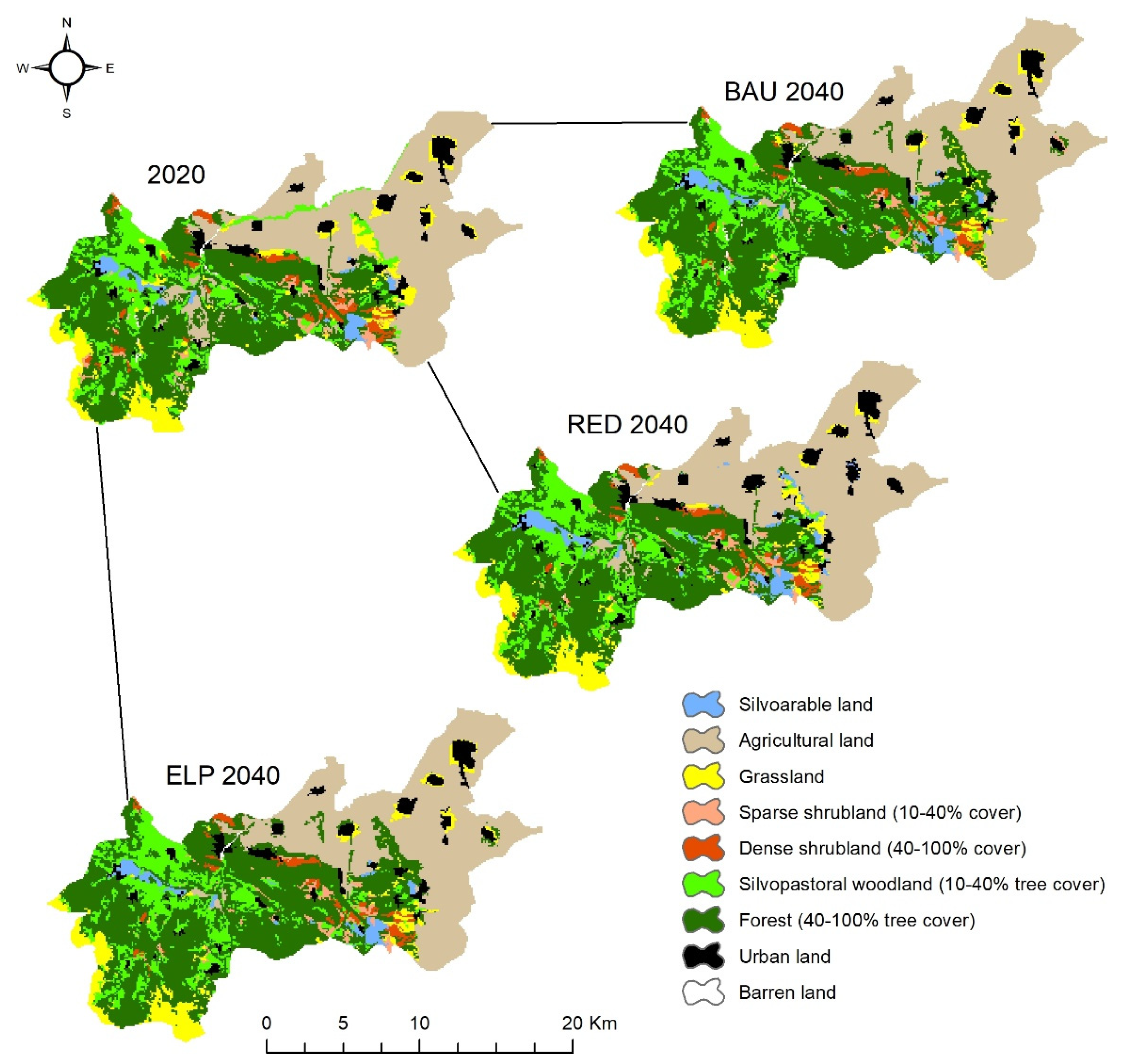
4.3. Implementation of Socioeconomic Scenarios

The spatiotemporal model CLUE-S completed the process of modeling the land use changes in the landscape of Mouzaki after the completion of the data supply in its spatial and non-spatial (socio-economic) modules. This took place for each of the three socio-economic scenarios (BAU, RED, and ELP) and in this way the corresponding final forecasting grid maps were produced (Figure 6), and areal data for each land use unit are presented in Table 5. The simulation of the land use changes showed that under the RED scenario, in the year 2040 the extent of the silvoarable systems was expected to increase significantly (+57%) compared to the reference year 2020, something that was also expected to happen under the BAU scenario, but to a much lesser extent (+14% approximately). The BAU and ELP scenarios predicted a reduction of the area of dense shrubs and grasslands by approximately 22% and 18%.

5. Discussion

The present study focused on the research of Agroforestry in Thessaly, in order to be a potential are of regional development by reforming the typical, intensified, and one-dimensional models of monocultures found in the region (Mylopoulos et al. [47]). For example, the extensive use of water-consuming crops, such as the cultivation of cotton in the area, has led to significant environmental degradation, both with the lowering of the underground aquifer and also due to the high agrochemical burden required by intensive cultivation and consequent production. In fact, as has been shown recently, this intensification has led to the depletion of a significant portion of the soil nutrients, resulting in severe soil degradation and abandonment, which in combination with climate change, now leads irreversible desertification of the agricultural lands in the Thessaly plain (Danalatos et al. [48]).
CLUE-S modeling was used as a means of spatiotemporal projection in 2040 of the land use units of the rural landscape of Mouzaki, including traditional Agroforestry (silvoarable and silvopastoral woodland systems), which were developed with the support of three socio-economic scenarios. Mouzaki is a typical, representative administrative unit for the region of Thessaly (Nasiakou [49]), and the results of the present research are expected to have wider validity at the regional level.

5.1. Scenario Analysis

The chosen socio-economic scenarios do not deal exclusively with the promotion and introduction of Agroforestry in the Thessaly plain, but rather represent real prospects of all land uses. The business as usual (BAU) scenario configures the linear projection of the current state as displayed from 1960 onwards. It is a feasible scenario given the area’s land use history (historical trend scenario) and is a commonplace in spatial-temporal landscape change research (e.g., Samie et al. [50] for rural Pakistan, Larbi et al. [51] for Ghana, Zhu et al. [52] for China). It is predicted that by 2040 there will be a significant increase in land use units that incorporate woody components (forests, woodland, and forest grassland systems). This evolution of the woody land units can be justified by the existing socioeconomic forces whose action prevents the intense use of agricultural/forest land by the inhabitants, both in the lowland areas of the central part of Mouzaki (mainly silvioarable areas), and of semi-mountainous and mountainous areas (mainly silvopastoral woodlands). It should be noted that the silvopastoral systems in 2040 will have the current traditional character of abandonment and in no case will they be organized systems, regularly maintained, or with the ultimate goal of harvesting the woody elements at the end of rotation time. In addition, the increase of silvoarable systems will occur as a result of the abandonment of mainly agricultural crops, as common practice has shown that farmers usually firstly abandon the treatment of the woody component in silvoarable systems if necessary. This is because trees have much longer margins of resistance to external pressures on crops. For example, the largest percentage (63%) of farmers (n = 111) surveyed on forestry farms in Mindanao, Philippines said they would abandon the timber component first if it had to abandon the silvoarable system where timber component belongs (Cenas and Pandey [53]). This is evident in the landscape of the mountain villages of Mouzaki, as the plantations with important woody species present in their majority a picture of abandonment, while areas of solely agricultural cultivation have usually been turned into an abandoned field (Nasiakou [49]).
The characteristics of agricultural land abandonment projected by the BAU scenario are very prevalent in south Mediterranean Europe. From the middle of the 20th century onwards, large areas of agricultural land have been abandoned. Although there is relatively little literature on the spatiotemporal characteristics of abandonment, the available data show that it is one of the most important land changes (Van der Sluis et al. [54,55]). In particular, in Spain it is expected that by 2030 an agricultural area equal to 1096.5 MHa will be abandoned, in France 625.1 MHa, in Italy 456.3 MHa, and in Greece 179.2 M Ha (Perpiña et al. [56]). For Greece, this abandoned area projected for 2030 is in line with the general trend of decreasing arable land according to data of the World Bank, where 3057 MHa of land in 1963 decreased to 2137 MHa in 2018, a decrease in the order of 30%.
Under BAU scenario the process of abandonment occurs largely as a result of the reduction of the viability of agricultural practices, which occurs mainly in remote and mountainous areas that are widespread, but also in semi-arid areas and even in fertile soils. It is influenced by a complex range of environmental, structural, and mainly socio-economic factors, often local and regional (Van der Sluis et al. [54]). Especially in arid areas, the projected effects of climate change will increase the risk of land abandonment. Land abandonment as a key regional environmental factor has significant implications for the environment and biodiversity. On the one hand, land abandonment can be considered beneficial, as it allows large-scale and low-cost restoration of forest habitats. It seems that rewilding is a natural trend in the European Mediterranean (Pointereau et al. [57], Herrando et al. [58]). However, land abandonment results in the degradation of agricultural land and the disappearance of semi-natural habitats, some of which are very important for biodiversity, such as semi-natural grasslands, pseudo-steppe, or silvopastoral systems (Herrando et al. [58], Russo [59], Tarolli and Straffelini [60]). Many of these habitats depend on High Natural Value agricultural systems, most of which are characterized by very marginal economic viability due to their low productivity and/or remote location (Keenleyside et al. [61]). Land abandonment can also affect biodiversity by accumulating biomass, which fuels fires, accelerating soil erosion, and landslides. In addition, abandonment can lead to the loss of cultural heritage and traditional forms of land management, such as Agroforestry.
The ecological land protection (ELP) scenario focuses on ensuring the highest naturalness of land types and is relevant to the BAU scenario. Achieving the goal of maximum naturalness is expected to lead to the preservation of traditional forestry systems and reduce the area of agricultural crops. Agroforestry systems bring significant environmental benefits associated with beneficial effects on the soil, tackling disease spread and microclimate modification (Le Houérou [62], Tuomisto et al. [63], and Ollinaho and Kröger [64]). Under this scenario there is a significant reduction of barren land, mainly due to the gradual emergence of natural succession (Gaxiola et al. [65]).
The goal of the rapid economic development (RED) scenario is to maximize the economic benefits that different units of land uses will produce for 2040. The development of the RED scenario is usually accompanied by an increase in the size of settlements/urban centers. For example, the implementation of a rapid economic growth scenario in the Punjab province of Pakistan, with the development of the DLS model, predicted a significant increase in the area of settlements (44.3%) for the year 2030 compared to 2010 (Samie et al. [50]). Accordingly, Wang et al. [39], during the implementation of the Dyna-CLUE model under the RED scenario, predicted for the year 2030 a significant increase (57.88%) of the area of Wuhan city, China compared to 2015. The implementation of the rapid economic growth (RED) scenario in the area of Mouzaki under the CLUE-S model predicted for the year 2040 an increase in the area of settlements by 15.71% compared to 2020, an increase less than those predicted by Samie et al. [50] and Wang et al. [39] for some regions of Pakistan and China, respectively. This differentiation can be attributed to the very high rates of population growth, the prevailing political conditions, the astyphilia, and the very intense pressures to find housing in urban centers that is observed in these countries (Jabeen et al. [66], Xiao et al. [67]).
The most characteristic change from the implementation of the rapid economic growth (RED) scenario comes from the projected increase in the area of silvoarable systems by 57% in the year 2040 compared to the reference year (2020). This increase is combined with changes observed in land use areas with woody components, and are expressed either by a reduction in their area, such as in dense shrubland, or by conservation of the area, such as in forest. In addition, there is a decrease in the areas of grasslands, while that of agricultural crops remains stable.

5.2. Investment on Agroforestry

It is a fact that rapid economic growth is accompanied by an increase in investment in all sectors of the economy and especially in the wider agricultural sector, given the general nature of the economy (Zepeda [68], FAO [69]). Particularly for Europe, Agroforestry is emerging as a well-promised practice of rural landscape redesign, and therefore financially promoted and supported by the CAP (Augère-Granier [70]). European farmers applying Agroforestry practices can receive direct payment per ha, as well as support for the establishment or maintenance of agroforestry systems under the CAP’s Rural Development tool. In addition, innovation and research conducted in this area are supported. The European Parliament has from time to time recognized the benefits of Agroforestry in various resolutions (indicatively, Resolution 2014/2223(INI), Resolution 2015/2226(INI) and Resolution 2018/2037(INI)), and has called for more effective support for a number of sustainable production methods, including Agroforestry. The promotional base of the Agroforestry-related entrepreneurship has already been demonstrated by the particular high synergy effect that characterizes it - the combination of many components and their dynamic interaction - that increases the overall productivity of the system. Researchers at INRA in France measure the productivity of an Agroforestry system using the Equivalent Land Ratio (LER), which compares yields from the cultivation of two or more components (crops, trees, animals) to yields from the cultivation of the same components individually, proved that the production from 1 Ha of the walnut/wheat combination is equal to that obtained from 1.4 Ha with separate tree crops (walnut plantations) and underlying crops (cereals) (Dupraz and Talbot [71]).
Investments in modern Agroforestry have already been proposed as a practice of ensuring long-term profit in many cases. Felker and Guevava [72] proposed investments in agroforestry systems of legumes and hardwood plantations (Prosopis alba) in Argentina, as they have an Internal Rate of Returns (IRR) ranging from 11.8% to 34.8% (depending on management practices) compared to just 5.3% obtained from an unmanaged monoculture of the hardwood species. The World Bank in Nairobi, Kenya, highlighted the benefits of investing in agroforestry in May 2011. A special forum was set up with the participation of the World Bank, IUCN and the WAC, with the aim of activating private investment in technology, based on tree plantations (Agroforestry) and the restoration of the environment in sub-Saharan Africa (PROFOR [73]). The growing potential for profit from investments in modern Agroforestry techniques has been demonstrated in the case of Brazil (Batista et al. [74]). In fact, Batista et al. [75] have developed a special application that calculates the economic figures resulting from investments in reforestation and in the installations of modern agroforestry systems. Faruqi et al. [76], in a case study, analyzed the financial profiles of 14 agroforestry holdings from eight countries and concluded that the opportunities created for profitable investments in Agroforestry are very large and promising.
However, investment in Agroforestry according to the World Bank [13] is associated with various obstacles, such as “high interest rates, unclear institutional framework, limited policy framework, poorly developed markets, and insufficient research and applications.” In addition, as Ollinaho and Kröger [64] have rightly pointed out, great care must be taken when investing in Agroforestry promotions so that the new emerging land use is not promoted as a business solely for economic gain (agrobizforestry, as they call it) which can often be combined with extensive alterations in the forest character of the land (agrodeforstry), but include social and environmental benefits (agroecoforestry). All these obstacles and concerns should be addressed effectively when designing flexible investment plans. According to Nasiakou [4] and Vrahnakis et al. [77], tackling many of these limiting factors and concerns can be organized with the input of business consulting companies investing in Agroforestry.

5.3. EU CAP and Investment in Agroforestry

The two most important financial instruments that significantly facilitate investment in Agroforestry in the EU are the Agri-Environmental and Climate Measures (AECMs) and the ecoschemes currently available through Pillar I and II of CAP, both of which are quite common characteristics. However, ecoschemes are part of Pillar I and are therefore fully funded from the EU budget. Ecoschemes’ payments are granted per Ha, as compensation for additional costs or lost income caused by the adoption of more environmentally friendly practices or as fixed additional payments to basic income support payments. This second option brings to the light the implementation of Payments for Ecosystem Services (PES) for the support that farmers have to receive due to climate change mitigation and environmental services offered by their systems. However, the PES will be determined essentially on the basis of farming practices (i.e., with a commitment to resources) and not on the basis of climatic and environmental benefits (i.e., a commitment of results) (Nasiakou [49]).
AECMs also aim to upgrade the rural environment from a more environmental-friendly perspective. They generally focus on (a) reversing biodiversity loss, (b) tackling (in the broadest sense) climate change, (c) protecting genetic resources, (d) conserving the landscape, (e) protecting water, and (f) protecting soil (Sulima [78]). Two approaches can be distinguished in AECMs: (a) the compliance-oriented one, where management practice is the central issue of a Measure and (b) the results-based one. There are challenges associated with both. Compliance-oriented is the dominant approach in which the planning of commitments, farmers’ activities, and eligibility rules are based on reasonable assumptions that the desired results may be achieved. These hypotheses must be supported by scientific or practical evidence (Scheele [79]). According to the results-based approach, it is difficult to calculate and justify the level of payments to farmers, as production methods are not defined in advance. Regardless of the approach used in an AECM, payment rates should be based on calculations of lost income and additional costs.
The adoption of ecoschemes and AECMs related to Agroforestry should be part of the Strategy for Rural and, therefore, for Regional Development, developed by each member state of the EU. Such a Strategy has been designed and implemented in many central European countries. However, Greece has not yet adopted in their fullness, despite the fact that the benefits of Agroforestry have full recognition scientifically, socially and economically. This has given impetus to many institutions either at the state level or an association of states to adopt and strengthen the application of Agroforestry in the wider rural area. The EU’s CAP has been moving towards this goal of promoting Agroforestry since the 2007–2013 programming period, when its forecasts were incorporated into the Rural Development Programs of Portugal, Spain and France, while Italy followed in the period 2014–2020.
The new CAP for the programming period 2021–2027 aims to promote a sustainable and competitive agricultural sector that can support farmers’ livelihoods and provide sustainable food for society, as well as for the revitalization of rural areas. The new CAP is expected to be a key tool in achieving the From Farm to Fork Strategy and the European Biodiversity Strategy 2030, two emblematic institutional efforts within EU’s Green Deal, and will play a key role in managing the transition to sustainable agriculture, towards a sustainable food system and to strengthening the efforts of European farmers to contribute to the EU’s goals related to climate change and environmental protection.

5.4. Limitations of the Research

CLUE-s is a valuable tool to model land use change as it is adequate enough for the demands for spatial and non-spatial integration. According to Briassoulis [20], it serves primarily as a predictive tool in analyzing land use impacts under socioeconomic scenarios at several geographic scales, and it is also simple to comprehend and easy to use. However, the statistical procedures do not rely on causal relationships, the analysis applied cannot capture the qualitative aspects of land uses change in relation to their cultural, political, and institutional nature, and the statistical importance of independent variables often does not asset their theoretical importance. According to the same author, the most prominent limitations stem from the lack of a theoretical basis able to sustain the modeling effort. Despite these inherent limitations, the prediction power of CLUE-s is great enough and is strongly suggested as supporting tool to land policy planning. For example, in the case of Lagadas district (Greece) the CLUE-S model estimated that the simulated area of grasslands will be reduced from years 1945 to 2013 almost to extinction (−95.69%) (Chouvardas and Vrahnakis [80]). In this case, the predictions of the CLUE-S model have recently been verified, since the real change of grassland area from 1945 to 2020 was reduced by 87.78% (Chouvardas et al. [81]). Finally, for Greece, the current institutional environment does not favour the application of or investments in Agroforestry, since the state’s Regional Development Strategy within the reformed CAP 2021–2027 excluded Agroforestry from payments. However, given the associated environmental and socioeconomic benefits, it is believed that soon this Strategy will change in favour of Agroforestry.

6. Conclusions

Particularly for the heavily environmentally burdened plain of Thessaly, Agroforestry stands out as an alternative option which is linked beyond the environmental benefit with significant socio-economic benefits. Its integration into farming practices is now a direct demand. In relation to the foreseen changes in the rural landscape of the modeled area of Mouzaki, it appears, according to the spatiotemporal model CLUE-S, that the silvoarable systems are expected to expand under the three scenarios. The scenario that favors this the most is that of rapid economic development (RED). In contrast, silvopastoral woodland in the mountains appears to remain stable, with only a small increase under the business as usual scenario (BAU). The RED scenario is associated with an increase in investments in innovative biological technologies, such as silvoarable systems. The use of EU CAP tools that are directly related to the promotion of Agroforestry, and especially ecoschemes and agri-environmental and climate measures, create a safe institutional environment for investments in Agroforestry in EU countries. Speaking in a broader context, economic development together with investments in Agroforestry within a favorable agro-policy framework offer the opportunity to establish agroforestry systems and exploit all the associated socio-economic and environmental benefits. These opportunities may be used as barriers to withhold the accelerating depopulation processes that occur in several countries of European south, and elsewhere. In this sense, EU countries must adopt Agroforestry in their Rural Development Strategy within CAP 2021–2027 as an innovative biological tool to create value for rural societies the and natural environment.

Author Contributions

Conceptualization, S.N., M.V. and V.K.; methodology, D.C., M.V., G.M., S.N. and V.K.; software, D.C.; validation, G.M., M.V., D.C., S.N. and V.K.; formal analysis S.N., M.V., D.C., G.M. and V.K.; investigation, S.N., G.M., M.V., D.C. and V.K.; resources, G.M., M.V. and D.C.; data curation, S.N., D.C., G.M., M.V. and V.K.; writing—original draft preparation, S.N., M.V., G.M. and D.C.; writing—review and editing, M.V., D.C., S.N., G.M. and V.K.; visualization, S.N., M.V., D.C., G.M. and V.K.; supervision, S.N. and M.V.; project administration, V.K.; funding acquisition, V.K. All authors have read and agreed to the published version of the manuscript.

Funding

This research was funded by the General Secretariat for Research and Innovation (GSRI) and the Hellenic Foundation for Research and Innovation (HFRI) with funding number 2610, and “The APC was funded by the General Secretariat for Research and Innovation (GSRI) and the Hellenic Foundation for Research and Innovation (HFRI)”.

Data Availability Statement

Data and material is available upon request.

Acknowledgments

The present study is part of the Ph.D. dissertation “Agroforestry and Regional Development: Policy and Economy Perspectives” conducted by Stamatia Nasiakou. The PhD and the present study were supported by the project entitled “Perspective of Agroforestry in Thessaly region: A research on social, environmental and economic aspects to enhance farmer participation”. The project was funded by the General Secretariat for Research and Technology (GSRT) and the Hellenic Foundation for Research and Innovation (HFRI).

Conflicts of Interest

The authors declare no conflict of interest.

References

  1. Schultz, T.W. Economic Growth and Agriculture; McGraw-Hill: New York, NY, USA, 1968. [Google Scholar]
  2. Hayami, Y.; Ruttan, V.W. Induced Innovation in Agricultural Development; Center for Economic Research, Department of Economics, University of Minnesota: Minnesota, MN, USA, 1971. [Google Scholar]
  3. Jin, H.; Jorgenson, D.W. Econometric modeling of technical change. J. Econom. 2010, 157, 205–219. [Google Scholar] [CrossRef]
  4. Nasiakou, S. Business Model Identification and Perceptions for Agroforestry Consulting Co. Master’s Thesis, Staffordshire University, Staffordshire, UK, 2013; p. 116. [Google Scholar]
  5. George, S.J.; Harper, R.J.; Hobbs, R.J.; Tibbett, M. A sustainable agricultural landscape for Australia: A review of interlacing carbon sequestration, biodiversity and salinity management in agroforestry systems. Agric. Ecosyst. Environ. 2012, 163, 28–36. [Google Scholar] [CrossRef]
  6. De Baets, N.; Vézina, A.; Gariépy, S. Portrait of Agroforestry in Quebec; PFRA, Regional Services, Quebec Region Agriculture and Agri Food Canada: Quebec City, QC, Canada, 2007. [Google Scholar]
  7. Stainback, G.A.; Masozera, M.; Mukuralinda, A.; Dwivedi, P. Smallholder agroforestry in Rwanda: A SWOT-AHP analysis. Small-Scale For. 2012, 11, 285–300. [Google Scholar] [CrossRef]
  8. Neyra-Cabatac, N.M.; Pulhin, J.M.; Cabanilla, D.B. Indigenous agroforestry in a changing context: The case of the Erumanen ne Menuvu in southern Philippines. For. Policy Econ. 2012, 22, 18–27. [Google Scholar] [CrossRef]
  9. Islam, K.K.; Hoogstra-Klein, M.; Ullah, M.O.; Sato, N. Economic contribution of participatory Agroforestry program to poverty alleviation: A case from Sal forests, Bangladesh. J. For. Res. 2012, 23, 323–332. [Google Scholar] [CrossRef]
  10. Ren, H.; Lu, Y.; Liu, C.; Meng, Q.; Shi, Y. Eco-environment contribution of Agroforestry to agriculture development in the plain area of China--Huai’ an prefecture, Jiangsu province as the case study area. J. Environ. Sci. (China) 2005, 17, 327–331. [Google Scholar]
  11. Nasiakou, S.; Vrahnakis, Μ. Agroforestry—Development prospects for Greece during the Economic Crisis. In Scientific Annales of Department of Forestry and Management of Environment and Natural Resources; Democritus University of Thrace: Orestiada, Greece, 2015; pp. 212–232. [Google Scholar]
  12. Streed, E. Identifying benefits in agroforestry extension. Agrofor. Adv. 1999, 2, 1–9. [Google Scholar]
  13. World Bank. Agriculture Investment Sourcebook; The World Bank: Washington, WA, USA, 2005. [Google Scholar]
  14. Mamanis, G.; Vrahnakis, M.; Chouvardas, D.; Nasiakou, S.; Kleftoyanni, V. Land use demands for the CLUE-S spatiotemporal model in an agroforestry perspective. Land 2021, 10, 1097. [Google Scholar] [CrossRef]
  15. Veldkamp, A.; Fresco, L.O. CLUE: A conceptual model to study the conversion of land use and its effects. Ecol. Model. 1996, 85, 253–270. [Google Scholar] [CrossRef]
  16. Veldkamp, A.; Fresco, L.O. CLUE-CR: An integrated multi-scale model to simulate land use change scenarios in Costa Rica. Ecol. Model. 1996, 91, 231–248. [Google Scholar] [CrossRef]
  17. Turner, B.L., II; Skole, D.; Sanderson, S.; Fischer, G.; Fresco, L.; Leemans, R. Land-Use and Land-Cover Change; Science/Research Plan; IGBP Report No.35, HDP Report No.7; IGBP: Stockholm, Sweden; HDP: Geneva, Switzerland, 1995. [Google Scholar]
  18. Fischer, G.; Ermoliev, Y.; Keyzer, M.A.; Rosenzweig, C. Simulating the Socio-Economic and Biogeophysical Driving Forces of Land-Use and Land-Cover Change; WP-96-010; IIASA: Luxemburg, 1996. [Google Scholar]
  19. Lonergan, S.; Prudham, S. Modeling global change in an integrated framework: A view from the Social Sciences. In Changes in Land Use and Land Cover: A Global Perspective; Meyer, W.B., Turner, B.L., II, Eds.; John Wiley: New York, NY, USA, 1994; pp. 411–435. [Google Scholar]
  20. Briassoulis, H. Analysis of Land Use Change: Theoretical and Modeling Approaches, 2nd ed.; Loveridge, S., Jackson, R., Eds.; West Virginia University Research Repository: Morgantown, VA, USA, 2020. [Google Scholar]
  21. Rounsevell, M.D.A. Spatial Modeling of the Response and Adaptation of Soils and Land Use Systems to Climate Change—An Integrated Model to Predict European Land Use (IMPEL). In Research Report for the European Commission, Framework IV Programme, Environment and Climate; Contract Nos. ENV4-CT95-0114 and IC20-CT96-0013; European Commission: Brussels, Belgium, 1999. [Google Scholar]
  22. Tobler, W. Cellular geography. In Philosophy in Geography; Gale, S., Olsson, G., Eds.; D. Reidel Publishing Company: Dordrecht, Germany, 1979; pp. 379–386. [Google Scholar]
  23. Veldkamp, A.; Fresco, L.O. Modeling land use dynamics by integrating bio-physical and human dimensions (CLUE) Costa Rica 1973–1984. Stud. Environ. Sci. 1995, 65, 1413–1416. [Google Scholar]
  24. Verburg, P.H.; de Konig, G.H.J.; Kok, K.; Veldkamp, A.; Fresco, L.O.; Bouma, J. Quantifying the Spatial Structure of Land Use Change: An Integrated Approach. In Proceedings of the Conference on Geo-Information for Sustainable Land Management, Wageningen University, Wageningen, The Netherlands, 17–21 August 1997. [Google Scholar]
  25. de Koning, G.H.J.; Veldkamp, A.; Verburg, P.H.; Kok, K.; Bergsma, A.R. CLUE: A tool for spatially explicit and scale sensitive exploration of land use changes. In Information Technology as a Tool to Assess Land Use Options in Space and Time; Stoorvogel, J.J., Borma, W.T., Eds.; Proceedings of an International Workshop: Lima, Peru, 1997. [Google Scholar]
  26. Verburg, P.H.; Soepboer, W.; Veldkamp, A.; Limpiada, R.; Espaldon, V.; Mastura, S.S.A. Modeling the spatial dynamics of regional land use: The CLUE-S model. Environ. Manag. 2002, 30, 391–405. [Google Scholar] [CrossRef]
  27. Verburg, P.H.; Overmars, K.P. Dynamic simulation of land-use change trajectories with the CLUE-S model. In Modelling Land-Use Change; Springer: Dordrecht, The Netherlands, 2007; pp. 321–335. [Google Scholar]
  28. de Koning, G.H.J.; Verburg, P.H.; Veldkamp, A.; Fresco, L.O. Multi-scale modelling of land-use change dynamics for Ecuador. Agric. Syst. 1999, 61, 77–93. [Google Scholar] [CrossRef]
  29. Salazar, E.; Henríquez, C.; Sliuzas, R.; Qüense, J. Evaluating spatial scenarios for sustainable development in Quito, Ecuador. Int. J. Geo-Inf. 2020, 9, 141. [Google Scholar] [CrossRef] [Green Version]
  30. Verburg, P.H.; Overmars, K.P.; Huigen, M.G.A.; de Groot, W.T.; Veldkamp, A. Analysis of the effects of land use change on protected areas in the Philippines. Appl. Geogr. 2006, 26, 153–173. [Google Scholar] [CrossRef]
  31. Schoorl, J.M.; Veldkamp, A.; Fresco, L.O.; Kok, K.; Verburg, P.H. The conversion of land use and its effects (CLUE): Modelling land use dynamics for Costa Rica and further development of the model. In Report of the UNEP/RIVM/PE workshop on Global and Regional Modeling of Food Production and Land Use; UNEP: Wageningen, The Netherlands, 1996; pp. 36–38. [Google Scholar]
  32. Verburg, P.H.; Veldkamp, A.; Bouma, J. Land use change under conditions of high population pressure: The case of Java. Glob. Environ. Chang. 1999, 9, 303–312. [Google Scholar] [CrossRef]
  33. Verburg, P.H.; Chen, Y.Q.; Veldkamp, A. Spatial explorations of land-use change and grain production in China. Agric. Ecosyst. Environ. 2000, 82, 333–354. [Google Scholar] [CrossRef]
  34. Chouvardas, D. Estimation of Diachronic Effects of Pastoral Systems and Land Uses in Landscapes with the Use of Geographic Information Systems (GIS). Ph.D. Thesis, School of Forestry and Natural Environment, Aristotle University of Thessaloniki, Thessaloniki, Greece, 2007. [Google Scholar]
  35. Verburg, P.H.; Veldkamp, A. Projecting land use transitions at forest fringes in the Philippines at two spatial scales. Landsc. Ecol. 2004, 19, 77–98. [Google Scholar] [CrossRef]
  36. Nasiakou, S.; Chouvardas, D.; Vrahnakis, Μ.; Kleftoyanni, V. Temporal changes analysis of Mouzaki’s landscape, western Thessaly, Greece (1960–2020). In Proceedings of the 10th Panhellenic Rangeland Congress, Florina, Greece, 2022. [Google Scholar]
  37. Rosenhead, J. Operational research in urban planning. Int. J. Manag. Sci. 1981, 9, 345–364. [Google Scholar] [CrossRef]
  38. Weintraub, A.; Bare, B.B. New issues in forest land management from an operational research perspective. Interfaces 1996, 26, 9–25. [Google Scholar] [CrossRef]
  39. Wang, Y.; Li, X.; Zhang, Q.; Li, J.; Zhou, X. Projections of future land use changes: Multiple scenarios-based impacts analysis on ecosystem services for Wuhan city, China. Ecol. Indic. 2018, 94, 430–445. [Google Scholar] [CrossRef]
  40. Mishra, M.K. Application of Operational Research in Sustainable Environmental Management and Climate Change; ZBW—Leibniz Information Centre for Economics: Kiel/Hamburg, Germany, 2020. [Google Scholar]
  41. Liu, J.; Huang, G.; Jia, P.; Chen, L. Improving herdsmen’s well-being through scenario planning: A case study in Xilinhot City, Inner Mongolia Autonomous Region. Geogr. Sustain. 2020, 1, 181–188. [Google Scholar] [CrossRef]
  42. Verburg, P.H. The CLUE Modeling Framework—The Conversion of Land Use and its Effects. In Manual for the CLUE-S Model; The CLUE Group, Department of Environmental Sciences, Wageningen University: Wageningen, The Netherlands, 2010. [Google Scholar]
  43. Soepboer, W. CLUE-S. In An Application for Sibuyan Island, The Philippines; Laboratory of Soil Science and Geology, Wageningen University: Wageningen, The Netherlands, 2001. [Google Scholar]
  44. Englesman, W.; Verburg, P.; Veldkamp, T.; Mastura, S. Simulating land use changes in an urbanising area in Malaysia. In An Application of the CLUE-S Model in the Selangor River Basin; Laboratory of soil Science and Geology, Wageningen University: Wageningen, The Netherlands, 2002. [Google Scholar]
  45. Mazzotti, F.; Vinci, J. Validation, Verification, and Calibration: Using Standardized Terminology When Describing Ecological Models; WEC216; Department of Wildlife Ecology and Conservation, UF/IFAS Extension, University of Florida: Gainesville, FL, USA, 2019. [Google Scholar]
  46. Pontius, R.G.; Schneider, L.C. Land-cover change model validation by an ROC method for the Ipswich watershed, Massachusetts, USA. Agric. Ecosyst. Environ. 2001, 85, 239–248. [Google Scholar] [CrossRef]
  47. Mylopoulos, N.; Kolokytha, E.; Loukas, A.; Mylopoulos, Y. Agricultural and water resources development in Thessaly, Greece in the framework of new European Union policies. Int. J. Riv. Bas. Manag. 2009, 7, 73–89. [Google Scholar] [CrossRef]
  48. Danalatos, Ν.; Giannoulis, Κ.; Bartzialis, D.; Skoufogianni, Ε.; Gkintsioudis, Ι. Issues and prospects of agriculture in Thessaly: Inclined lands. In Proceedings of the AgriBusiness Thessaly Summit 2021 “Future of the Plain of Thessaly in Digital Era”, Trikala, Greece, 19–20 November 2021. (In Greek). [Google Scholar]
  49. Nasiakou, S. Agroforestry and Regional Development: Policy and Economy Perspectives. Ph.D. Thesis, Department of Forestry and Management of the Environment and Natural Resources, Democritus University of Thrace, Orestiada, Greece, 2022. [Google Scholar]
  50. Samie, A.; Deng, X.; Jia, S.; Chen, D. Scenario-based simulation on dynamics of land-use-land-cover change in Punjab Province, Pakistan. Sustainability 2017, 9, 1285. [Google Scholar] [CrossRef] [Green Version]
  51. Larbi, Ι.; Forkuor, G.; Hountondji, F.C.C.; Agyare, W.A.; Mama, D. Predictive land use change under Business-As-Usual and afforestation scenarios in the Vea Catchment, West Africa. Int. J. Adv. Remote Sens. GIS 2019, 8, 3011–3029. [Google Scholar] [CrossRef]
  52. Zhu, B.; Zhu, X.; Zhang, R.; Zhao, X. Study of multiple land use planning based on the coordinated development of wetland farmland: A cases study of Fuyuan City, China. Sustainability 2019, 11, 271. [Google Scholar] [CrossRef] [Green Version]
  53. Cenas, P.A.A.; Pandey, S. Determinants of adoption and retention of contour hedgerows in Claveria, Misamis Oriental. Phil. J. Crop Sci. 1996, 211, 34–39. [Google Scholar]
  54. van der Sluis, T.; Kizos, T.; Pedroli, B. Landscape change in Mediterranean farmlands: Impacts of land abandonment on cultivation terraces in Portofino (Italy) and Lesvos (Greece). J. Landsc. Ecol. 2014, 7, 23–44. [Google Scholar] [CrossRef] [Green Version]
  55. van der Sluis, T.; Arts, B.; Kok, K.; Bogers, M.; Gravsholt Busck, A.; Sepp, K.; Loupa-Ramos, I.; Pavlis, V.; Geamana, N.; Crouzat, E. Drivers of European landscape change: Stakeholders’ perspectives through Fuzzy Cognitive Mapping. Landsc. Res. 2019, 44, 458–476. [Google Scholar] [CrossRef] [Green Version]
  56. Perpiña, C.; Kavalov, B.; Diogo, V.; Jacobs-Crisioni, C.; Batista e Silva, F.; Lavalle, C. Agricultural Land Abandonment in the EU within 2015–2030; JRC Policy Insights; JRC113718; European Commission: Brussels, Belgium, 2018. [Google Scholar]
  57. Pointereau, P.; Coulon, F.; Girard, P.; Lambottte, M.; Stuczynski, T.; Sánchez Ortega, V.; Del Rio, A. Analysis of farmland abandonment and the extend and location of agricultural areas that are actually abandoned or are in risk to be abandoned. In Institute for Environmental Sustainability; European Commission, Joint Research Centrer, ISPRA: Varese, Italy, 2008. [Google Scholar]
  58. Herrando, S.; Brotons, L.; Anton, M.; Páramo, F.; Villero, D.; Titeux, N.; Quesada, J.; Stefanescu, C. Assessing impacts of land abandonment on Mediterranean biodiversity using indicators based on bird and butterfly monitoring data. Environ. Conserv. 2016, 43, 69–78. [Google Scholar] [CrossRef] [Green Version]
  59. Russo, D. Effects of Land Abandonment on Animal Species in Europe: Conservation and Management Implications. In Report of Project “Integrated Assessment of Vulnerable Ecosystems under Global Change”; 5 EU Research Framework: Brussels, Belgium, 2006. [Google Scholar]
  60. Tarolli, P.; Straffelini, E. Agriculture in hilly and mountainous landscapes: Threats, monitoring and sustainable management. Geogr. Sustain. 2020, 1, 70–76. [Google Scholar] [CrossRef]
  61. Keenleyside, C.; Beaufoy, G.; Tucker, G.; Jones, G. High Nature Value farming throughout EU-27 and its financial support under the CAP. In Report Prepared for DG Environment, Contract No ENV B.1/ETU/2012/0035; Institute for European Environmental Policy: London, UK, 2014. [Google Scholar]
  62. Le Houérou, H.N. Agroforestry and sylvopastoralism to combat land degradation in the Mediterranean basin: Old approaches to new problems. Agric. Ecosyst. Environ. 1990, 33, 99–109. [Google Scholar] [CrossRef]
  63. Tuomisto, H.L.; Hodge, I.D.; Riordan, P.; Macdonald, D.W. Does organic farming reduce environmental impacts?—A meta-analysis of European research. J. Environ. Manag. 2012, 112, 309–320. [Google Scholar] [CrossRef]
  64. Ollinaho, O.I.; Kröger, M. Agroforestry transitions: The good, the bad and the ugly. J. Rural Stud. 2021, 82, 210–221. [Google Scholar] [CrossRef]
  65. Gaxiola, A.; McNeill, S.M.; Coomes, D.A. What drives retrogressive succession? Plant strategies to tolerate infertile and poorly drained soils. Funct. Ecol. 2010, 24, 714–722. [Google Scholar] [CrossRef]
  66. Jabeen, N.; Farwa, U.; Jadoon, Z.I. Urbanization in Pakistan: A governance perspective. In Proceedings of the Sydney International Business Research Conference, University of Western, Sydney, Australia, 17–19 April 2015. [Google Scholar]
  67. Xiao, Y.; Song, Y.; Wu, X. How far has China’s urbanization gone? Sustainability 2019, 10, 2953. [Google Scholar] [CrossRef] [Green Version]
  68. Zepeda, L. Agricultural Investment and Productivity in Developing Countries. In FAO Economic and Social Development Paper, No. 148; Food and Agriculture Organization: Rome, Italy, 2001. [Google Scholar]
  69. FAO. The Future of Food and Agriculture—Alternative Pathways to 2050; Food and Agriculture Organization: Rome, Italy, 2018. [Google Scholar]
  70. Augère-Granier, M.-L. Agroforestry in the European Union; European Parliamentary Research Service: Brussels, Belgium, 2020; p. 11. [Google Scholar]
  71. Dupraz, C.; Talbot, C. Evidences and explanations for the unexpected high productivity of improved temperate agroforestry systems. In Proceedings of the 1st EURAF Conference, Brussels, Belgium, 9 October 2012. [Google Scholar]
  72. Felker, P.; Guerava, J.C. Potential of commercial hardwood forestry plantations in arid lands—An economic analyses of Prosopis lumber production in Argentina and the United States. For. Ecol. Manag. 2003, 186, 271–286. [Google Scholar] [CrossRef]
  73. PROFOR. Investing in Trees and Landscape Restoration in Africa: Overview; Program for Forests (PROFOR): Washington, DC, USA, 2011. [Google Scholar]
  74. Batista, A.; Calmon, M.; Lund, S.; Assad, L.; Pontes, C.; Biderman, R. Investing in Native Trees and Agroforestry Systems in Brazil: An Economic Evaluation; WRI Brazil: Porto Alegre, Brazil, 2021. [Google Scholar]
  75. Batista, A.; Prado, A.; Pontes, C.; Matsumoto, M. Verena Investment Tool: Valuing Reforestation with Native Trees and Agroforestry Systems; Technical Note; WRI Brazil: Porto Alegre, Brazil, 2017. [Google Scholar]
  76. Faruqi, S.; Wu, A.; Anchondo Ortega, A.; Batista, A.; Brolis, E. The Business of Planting Trees: A Growing Investment Opportunity; WRI, The Nature Conservancy: Washington, DC, USA, 2018. [Google Scholar]
  77. Vrahnakis, Μ.; Nasiakou, S.; Kazoglou, Y.; Blanas, G. Business model for agroforestry consulting company. Agrofor. Syst. 2016, 90, 219–236. [Google Scholar] [CrossRef]
  78. Sulima, K. Agri-Environment-Climate Measures: Support for Results, Controllability and the Way to Go? In Proceedings of the European Network for Rural Development, Workshop on Agri-Environment-Climate Measures (AECM): Challenges of Controllability and Verifiability, Brussels, Belgium, 7 December 2016. [Google Scholar]
  79. Scheele, Μ. Welcome Note. In Proceedings of the European Network for Rural Development, Workshop on Agri-Environment-Climate Measures (AECM): Challenges of Controllability and Verifiability, Brussels, Belgium, 7 December 2016. [Google Scholar]
  80. Chouvardas, D.; Vrahnakis, M.S. A semi-empirical model for the near-future evolution of the lake Koronia landscape. J. Environ. Prot. Ecol. 2009, 10, 867–876. [Google Scholar]
  81. Chouvardas, D.; Karatassiou, M.; Tsividis, I.; Palaiochorinos, S. Study of spatio-temporal changes (1945–2020) in a grazed landscape of northern Greece, in relation to socioeconomic changes. In Proceedings of the Hybrid workshop: Territorial Changes and Livelihood Transformations: Agro-pastoral Communities Living with Uncertainties in Dryland Settings, Market Integration, Livelihood Mobility, Land-Use Changes, European University Institute, Florence, Italy, 25–26 November 2021. [Google Scholar]
Figure 1. Land use map of Municipality of Mouzaki, Thessaly, Greece for 2020.
Land 11 00598 g001
Figure 2. Eastern lowland areas of the landscape of Mouzaki, where the conversion of grassland into forest is not permissible, as reflected in the matrix of permissible transformations.
Land 11 00598 g002
Figure 3. Flow chart representing the processes between spatial and non-spatial modules of CLUE-S.
Land 11 00598 g003
Figure 4. Landscape of Mouzaki. Spatial distribution of elevation classes (m, A), slopes (%, B), parent rock and soil depth (C), erosion potential (t/Ha/year, D), distances from road network (m, E), distances from hydrological network (m, F), distances from urban centers (m, G), inhabitant density (inh./Ha, H), sheep density (head/Ha, I), and goat density (head/Ha, J).
Land 11 00598 g004
Figure 5. Probability maps for major land use units of the landscape of Mouzaki. Light-colored areas indicate places with a higher probability of occurrence: (A) Silvoarable (0 to 99%), (Β) Agricultural land (0 to 99%), (C) Grassland (0 to 99%), (D) Sparse shrubland (0 to 62%), (Ε) Dense shrubland (0 to 71%), (F) Silvopastoral woodland (0 to 99%), (G) Forest (0 to 100%), and (H) Settlements (0 to 92%).
Land 11 00598 g005
Figure 6. Forecast map of the landscape changes of Mouzaki for the period 2020–2040 (all forecast scenarios), after CLUE-S.
Land 11 00598 g006
Table 1. Independent variables, type, unit of measurement, and data source for the supply of CLUE-S during the modeling of land use changes of the landscape of Municipality of Mouzaki, Thessaly, Greece.
a/aIndependent Variables *Type/UniteData Source
1Elevation zones Continuous/mDEM Aster 2
2SlopesContinuous/%DEM Aster 2
3Alluvial deposits/Very deep soilsBinary/0–1Soil map (Nakos 1991)
4Limestone/Medium -Shallow to rocky soils>> >>
5Flysch/Deep soils>> >>
6Tertiary deposits/Deep to medium depth soils >> >>
7Peridotite-Gabbro/Medium depth soils>> >>
8Schist/Deep soils>> >>
9River bedrock/Rocky soils>> >>
10Erosion potentialContinuous/(t × Ha−1 × year−1)Soil Erosion by Water (RUSLE 2015)/ESDAC **
11Distance from road networkContinuous/mDigital files from State Cadastre, Google Earth
12Distance from hydrological network>> Hydrological model from DEM, topographic maps, Google Earth
13Distance from urban centres>> Land use map 2020
14Inhabitant density Continuous/Number × Ha−1 of the total areaOfficial State Data (statistics.gr)
15Sheep density>> Municipality services of Mouzaki
16Goat density>> >>
* Landscape driving factors. ** European Soil Data Centre.
Table 2. Land use categories and the values of their coefficient elasticity.
Land Use CategoriesCoefficient of Elasticity
Agricultural land0.5
Silvoarable land0.8
Grassland0.0
Silvopastoral woodland (10–40% tree cover)0.1
Forest (40–100% tree cover)0.5
Sparse shrubland (10–40% shrub cover)0.1
Dense shrubland (40–100% shrub cover)0.9
Urban land0.9
Barren land0.9
Table 3. Matrix of permissible transformations of the landscape of M. of Mouzaki (SA = Silvoarable, G = Grassland, AL = Agricultural land, SS = Sparse Shrubland, DS = Dense Shrubland, SW = Silvopastoral Woodland, F = Forest, ST = Settlements and BL = Barren Land).
SA (0)AL (1)G (2)SS (3)DS (4)SW (5)F (6)ST (7)BL (8)
SA (0)111111110
AL (1)11111111010
G (2)1111111610
SS (3)111111110
DS (4)000111110
SW (5)110001110
F (6)000000110
ST (7)000000010
BL (8)111111111
Table 4. Logistic regression coefficients (b-values), exp (b) (in parentheses), Relative Influence Index [in brackets] and AUC (Area Under the Curve). Only statistically significant coefficients appear, for significance level α = 0.02. (SA = Silvoarable, G = Grassland, AL = Agricultural land, SS = Sparse Shrubland, DS = Dense Shrubland, SW = Silvopastoral Woodland, F = Forest, ST = Settlements and BL = Barren Land).
Independent Variables *SAALGSSDSSWFSTBL
Elevation zones −0.0050.005−0.002−0.004−0.001 −0.001
(0.995)(1.005) (0.998) (0.996) (0.999) (0.999)
[−6086.3][7181.3][−33.45][−1114.5][−2.871][−14.17]
Slopes−0.043−0.084−0.009−0.0130.0120.007 0.018 0.076
(0.958) (0.920) (0.991) (0.987)(1.012) (1.007) (1.019) (1.079)
[−132.0][−12,296.5][−2.674][−4.427][3.699][2.138][7.942][5288.5]
Alluvial deposits/Very deep soils1.4282.4251.828 −2.513−3.745 3.352
(4.169) (11.30) (6.223) (0.081)(0.024)(28.57)
[4.169][11.30][6.223][−12.34][−42.31][28.57]
Limestone/ Medium—Shallow to rocky soils 5.4487.792 −0.531
(232.2) (2420.5) (0.588)
[232.2][2420.5][−1.700]
Flysch/Deep soils 2.2270.8911.8016.8110.926 −1.474
(9.276) (2.438) (6.057) (907.6) (2.524)(0.229)
[9.276][2.438][6.057][907.6][2.524][−4.368]
Tertiary deposits/Deep to medium depth soils 1.737 3.1694.1806.964−1.081 −0.807
(5.678)(23.79) (65.35) (1058.1) (0.339)(0.446)
[5.678][23.79][65.35][1058.1][−2.947][−2.241]
Peridotite-Gabbro/Medium depth soils 7.0328.260
(1132.5) (3867.9)
[1132.5][3867.9]
Schist/Deep soils 1.869−0.999 4.609
(6.483) (0.368) (100.4)
[6.483][−2.715][100.4]
River bedrock/Rocky soils 1.006 −1.643 4.714
(2.734)(0.193)(111.5)
[2.734][−5.171][111.5]
Erosion potential0.0270.023 0.020 0.027 −0.015 0.021
(1.027)(1.023)(1.020)(1.028)(0.985) (1.021)
[158.0][78.39][42.79][173.2][−17.51][55.19]
Distance from road network −0.001 0.002 0.006
(0.999) (1.002)(1.006)
[−3.520][9.924][8932.9]
Distance from hydrological network−0.0010.001 0.0010.001 −0.001 −0.002
(0.999) (1.001) (1.001) (1.001) (0.999)(0.998)
[−8.288][2.423][4.146][3.996][−3.234][−15.21]
Distance from urban centres−0.0010.001 0.000 0.000 0.003 −0.006
(0.999) (1.001) (1.000) (1.000)(1.003)(0.994)
[−365.2][471.9][6.235][−8.351][10,681,724.0][−5.0 × 10¹²]
Inhabitant density −4.9550.2810.692−2.358(1.000)−0.546 −0.904 1.009
(0.007) (1.325) (1.999) (0.095) (0.579)(0.405)(2.744)
[−12,114.4][1.706][3.721][−87.81][−2.820][−5.558][6.788]
Sheep density(1.000)1.1080.4680.2710.3750.431 −28.026 −18.535 −32.210
(3.029)(1.596) (1.311) (1.455) (1.539)(0.000)(0.000)(0.000)
[1101.4][19.22][5.546][10.69][15.25][−8.4 × 1076][−7.5 × 1050][2.6 × 1088]
Goat density1.711−2.220 0.9970.652 0.859 −35.78 −27.80
(5.532)(0.109)(2.709) (1.920) (2.361)(0.000)(0.000)
[81.14][−300.2][12.95][5.345][9.097][−8.5 × 1039][−1.1 × 1031]
Constant−2.265−2.970−6.766−7.273−9.948 −1.624 0.581 2.461 −8.512
(0.104)(0.051)(0.001)(0.001)(0.000)(0.197)(1.787)(11.71)(0.000)
AUC0.9390.9680.8350.9370.9230.8670.9970.9820.946
* Landscape driving factors.
Table 5. Area distribution (Ha) and rate of change (%) of land use units of Mouzaki for the period 2020–2040 for all socio-economic scenarios (BAU, RED, ELP).
Land Use2020BAU 2040RED 2040ELP 2040
Silvoarable565645 (+14.16%)887 (+56.99%)557 (−1.42%)
Agricultural land11,14810,358 (−7.09%)11,149 (+0.01%)10,344 (−7.21%)
Grassland24211990 (−17.80%)2044 (−15.57%)1990 (−17.80%)
Sparse shrubland503514 (+2.19%)503 (-)505 (+0.40%)
Dense shrubland782608 (−22.25%)611 (−21.87)609 (−22.12%)
Silvopastoral woodland38194003 (+4.82%)3819 (-)3818 (−0.03%)
Forest10,56111,682 (+10.61%)10,617 (+0.53%)12,036 (+13.97%)
Settlements14581458 (-)1687 (+15.71%)1458 (-)
Barren land9089 (−1.11%)30 (−66.67%30 (−66.67%)
Total (Ha)31,34731,34731,34731,347
Publisher’s Note: MDPI stays neutral with regard to jurisdictional claims in published maps and institutional affiliations.

