Article

Conservation Prioritization in a Tiger Landscape: Is Umbrella Species Enough?

1
Wildlife Institute of India, Chandrabani, Dehradun 24800, India
2
Faculty of Forestry, University of British Columbia, 2424 Main Mall, Vancouver, BC V6T 1Z4, Canada
3
School of Environmental and Forest Sciences, University of Washington, Seattle, WA 98195, USA
*
Author to whom correspondence should be addressed.
Land 2022, 11(3), 371; https://doi.org/10.3390/land11030371
Submission received: 8 February 2022 / Revised: 25 February 2022 / Accepted: 1 March 2022 / Published: 3 March 2022
(This article belongs to the Special Issue Decision Support Tools for Land Management)

Abstract

:
Conservation approaches in tiger landscapes have focused on single species and their habitat. Further, the limited extent of the existing protected area network in India lacks representativeness, habitat connectivity, and integration in the larger landscape. Our objective was to identify sites important for connected tiger habitat and biodiversity potential in the Greater Panna Landscape, central India. Further, we aimed to set targets at the landscape level for conservation and prioritize these sites within each district in the landscape as specific management/conservation zones. We used earth observation data to derive an index of biodiversity potential. Marxan was used to identify sites that met tiger and biodiversity conservation targets with minimum costs. We found that to protect 50% of the tiger habitat with connectivity, 20% of the landscape area must be conserved. To conserve 100% of high biodiversity potential, 50% moderate biodiversity potential, and 25% low biodiversity potential, 55% of the landscape area must be conserved. To represent both tiger habitat and biodiversity, 62% of the total landscape area requires conservation or restoration intervention. The prioritized zones can prove significant for hierarchical decision making, involving multiple stakeholders in the landscape, including other tiger range areas.

1. Introduction

Protected areas (PAs) are among the important strategies of target-based conservation approaches [1]. The PA network in India covers 5.03% of the geographical area and includes national parks, wildlife sanctuaries, community reserves, and conservation reserves [2]. PAs have made a significant contribution to the conservation of biodiversity in India [3]. A significant contribution to this network is made by the Tiger Reserve Network (often combines existing PAs—national parks, wildlife sanctuaries, and reserve forests), which covers ~2% of the geographical area of the country. Since the beginning of the Project Tiger in 1973, Tigers (Panthera tigris) have played the role of both flagship and umbrella species and aided forest conservation through enhanced legal protection under Wildlife (Protection) Act, 1972 [4,5,6,7,8]. Tiger reserves instantiate the integration of forest and wildlife conservation since tiger conservation relies on the quality of forest cover and characteristics of surrounding forest landscape such as landscape connectivity, prey population, and intensity of human disturbance. For tigers and large carnivores, their large body size, large home ranges, dispersal as an important life-history trait, endangered status, etc. fulfill some of the common agreed-upon characteristics of umbrella species [9,10,11]. The practical effectiveness of the umbrella species approach, in general, has been tested in a few studies, and there have been different experiences globally [12,13,14,15]. Its utility as a conservation tool has not been empirically tested in the case of tigers, but the umbrella species approach has been found to be more effective in selecting biologically important areas, as opposed to randomly selecting habitat patches for conservation [15], in addition to its higher efficacy in other cases to determine the size and type of habitats to protect [16].
The effectiveness of conservation efforts through PAs also depends on representativeness, connectivity, and integration of PAs in the larger landscape (Aichi Target 11) [1]. With fewer functional corridors connecting PAs in India, the surrounding human-use matrix plays an important role in the dispersal and movement of animals [17,18]. For the success of these species in the PAs, they must be surrounded by sustainably managed landscapes, mimicking an adaptive mosaic [19,20,21]. Further, PAs are not immune to downgrading, downsizing, degazettement, or other management issues [22,23]. The proposed Ken–Betwa Link Canal Project (KBLCP) in the central Indian landscape, for example, will submerge 90 km2 area and will also impact the connectivity with another 105 km2 of the core tiger habitat area of Panna Tiger Reserve (PTR) on the western side of the Ken River. Given the fact that PTR has recovered from a state of functional extinction of the tiger population in the recent past, the current and future management including human–wildlife interface issues ought to be seen and managed from these pragmatic perspectives. The issues concerning PTR and the surrounding areas that can be termed as “Greater Panna Landscape” (GPL), require an integrated landscape approach to ensure biodiversity conservation and well-being of the people in the long term. Therefore, we explore the idea for an integrated landscape management plan for this landscape further in this study, which originated as a part of the process for KBLCP.
GPL, centered around PTR in central India, is an important tiger habitat, with the latter as the major source population. It is a heterogeneous landscape—a mosaic of agriculture and forest. Conservation efforts have so far followed the top-down approach through protected area designation and intensive management within the PAs. While forest and wildlife conservation are intertwined and inseparable, they are often planned in silos through forest working plans, wildlife management plans, and tiger conservation plans, which makes it difficult to set comprehensive and inclusive conservation goals. For example, the surrounding forest patches and riverine ecosystems are important for dispersing tigers but also for other taxa such as the vultures and gharials (Gavialis gangeticus) [24,25]
PTR is now more known for the “fall and rise of the tiger” due to local extinction and subsequent successful reintroduction of the tiger. The Tiger population in the PTR during the 1980s was reported to be around 20 and remained in the range of 25–30 until 2000. Tiger number continued to decline, became functionally extinct by 2008, and it subsequently lost all its tigers in early 2009 [26]. To revive the tiger population, a concerted effort through a comprehensive recovery program was implemented by the Madhya Pradesh State Forest Department, supported by the Wildlife Institute of India (WII) and National Tiger Conservation Authority (NTCA), beginning in 2009 and continuing up till June 2021. From three translocated individuals in 2009 and subsequently another four over the years [27], the tiger population grew rapidly and reached beyond the estimated carrying capacity to the current population of around 60 individuals (as of 2021), much beyond the historically recorded number for the reserve. With the growing population, tigers have naturally dispersed from PTR and into the surrounding landscape, with an estimated 37 dispersal events. Therefore, the conservation of these tigers must be considered on the landscape scale.
Setting targets and prioritizing areas for tiger conservation has historically followed a species-centric approach at global, regional, and local scales. Conservation planning initiatives at the global level prioritized several representative tiger habitats across the tiger range countries through initiatives such as “A Framework for Identifying High-Priority Areas and Actions for the Conservation of Tigers in the Wild” (also known as TCU 1.0), and it identified tiger conservation units in different bioregions [28]. Habitat integrity, poaching pressure, and population status were the three key criteria in this ecological approach. A second version that was more objective and data-driven was “Setting Priorities for the Conservation and Recovery of Wild Tigers: 2005–2015” (also known as TCL 2.0), and it delineated tiger conservation landscapes [29]. Setting such priority areas and targets for conservation allowed focused allocation of resources to safeguard the inviolate areas and habitat protection with representation and redundancy. Tiger conservation planning at the national and regional level has also followed a similar ecological approach for identifying priority areas, for example, in Nepal and the Terai Arc landscape in India [30,31,32] assuming the umbrella effect of tiger species. Prioritization of conservation areas using this popular but somewhat controversial umbrella species approach [15] can be problematic in landscapes with several species of conservation importance [33]. Decision making and management with a focus on one species do not consider the differential impact of landscape change on the other species [34]. Further, habitat selection at a finer scale can be different for different species occupying the same region [35]. Therefore, a multiscale and multispecies conservation approach is essential.
Landscape approaches often involve assessment and planning at multiple scales [17,36,37,38,39]. At the landscape scale, connectivity for tigers, satellite cores, and stepping stones are important features to preserve, in addition to the biophysical features within the landscape [17,40]. For example, cliffs and deep gorges are the characteristic topographic features of GPL and are important for the conservation of vultures [24]. At finer scales, for example at the stand level, species richness, diversity, and nesting sites are some of the important features to preserve. Conservation of these features can be carried out through spatial prioritization by setting conservation targets. Based on the availability of data and objectives, past studies have set targets for features such as natural areas, species richness and diversity, geological and topographical features, vegetation types, and ecosystem services [41,42,43,44,45]. Data availability for species and their habitat is an important challenge to this approach, which can be overcome by earth observation data, which play important roles in computing taxonomic and environmental surrogates for conservation features in areas with no or insufficient field data [46,47,48,49,50].
GPL has been envisioned to protect and consolidate forest patches and biodiversity-rich areas around the PTR taking a landscape approach to wildlife conservation (National Wildlife Action Plan, 2017–2031). It was also envisioned to facilitate the conservation of the tiger in a metapopulation framework while conserving other focal species such as crocodiles and vultures, as well as the overall biodiversity of the area. In this study, we used earth-observation-based environmental surrogates (biodiversity potential) and habitat connectivity for tiger species to identify sites within the GPL that meet the broad conservation targets for the landscape using a reserve selection tool Marxan [51,52]. We further prioritized these identified sites by creating specific management/conservation zones based on various combinations of tiger habitat and biodiversity potential areas identified at five levels. The prioritization maps generated through this assessment can be used as baselines for stakeholder engagement and appropriate conservation practice in each district and can encourage the deliberative process of negotiations at the village, district, and landscape levels. This also allows the implementation framework to be integrated with the five-stage multilevel planning framework in India. In this context, our study offers a unique perspective on conservation prioritization, compared with other similar studies globally [53,54,55].

2. Materials and Methods
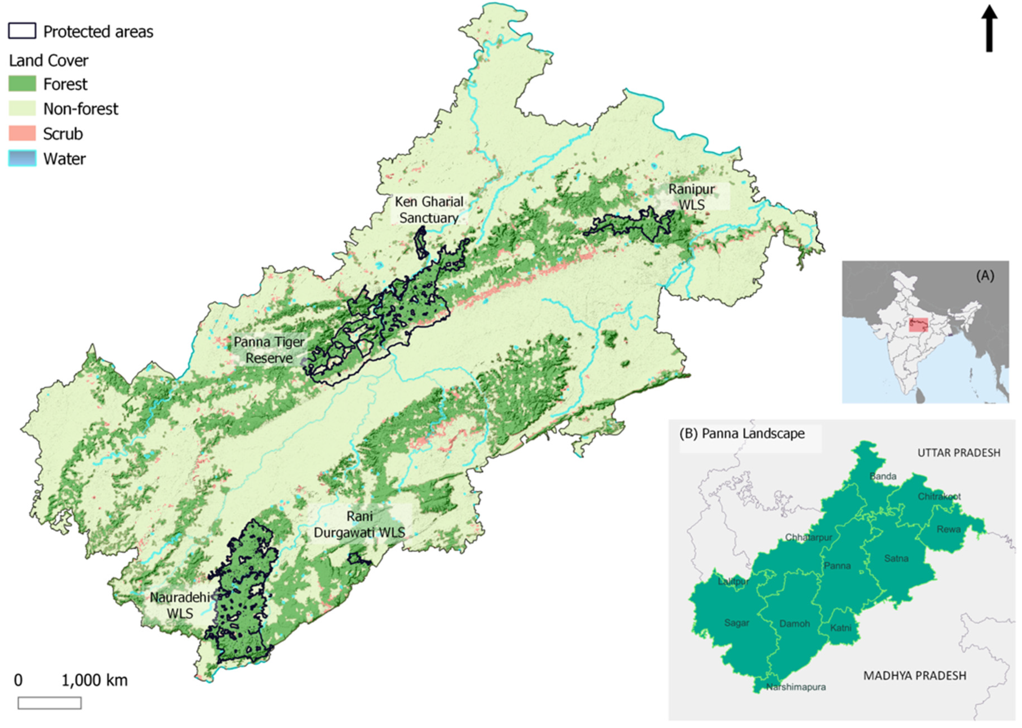
2.1. Study Area

The study was conducted in the Greater Panna Landscape in central India (Figure 1). The landscape was defined using the administrative boundary of 11 districts of 2 states—Uttar Pradesh and Madhya Pradesh. The extent of the landscape was decided by the extent of contiguous forest patches and protected areas around the Panna Tiger Reserve. It extends between 81°53′25.70″ E to 78°17′12.56″ E longitude and 24°53′13.77″ N to 24°14′4.78″ N latitude, with a total area of over 47,000 km2. There are five protected areas within Panna Landscape (Panna Tiger Reserve, Ranipur Wildlife Sanctuary, Veerangana Durgawati Sanctuary, Nauradehi Wildlife Sanctuary, Ken Gharial Sanctuary) and an Important Bird and Biodiversity Area (IBA) (Rangwana Reservoir). Protected areas make up approximately 6% of the geographical area of the GPL and 26% of the total forest cover of GPL. The landscape has a hot climate with three distinct seasons—summer, winter, and monsoon.

2.2. Data Collection and Mapping

2.2.1. Systematic Conservation Planning

Systematic Conservation Planning has been used widely in both terrestrial and marine ecosystems to design networks of reserves that conform to the representativeness of the biodiversity of the region and meet the “big-picture” conservation goals in an objective and transparent manner [56]. Marxan is a popular conservation planning software that was created to solve minimum set reserve design problems and answer questions such as “What is the minimum number of sites, or minimum total area, necessary to represent all species?” [56]. It has been used to identify restoration and conservation sites across the globe [41,42,43,44,45]. It uses simulated annealing as the optimization method to design reserves that meet the target (or a set of criteria) at the lowest cost [57]. This is accomplished by calculating the objective function value for a set of planning units (PUs) (out of the available planning units) that would become part of the reserve system. The lowest value of the objective function for any configuration of PUs indicates an efficient selection of PUs for the reserve system. An objective function constitutes a “cost” (e.g., economic cost) and a conservation feature penalty (or species penalty factor (SPF)) for not meeting the target for that conservation feature (Supplementary Information, Table S1). The objective function can be written as in Equation (1).
Score of the configuration being tested = (Σ Cost of PUs) + (BLM ×
Σ Boundary length) + (SPF × Penalty incurred for unmet targets)

2.2.2. Planning Area and Planning Units

For the present assessment, the planning area was the GPL. The landscape shapefile was created by merging the district polygons. The analysis was carried out using PUs of square grid cells of 4 km × 4 km for tiger and 2 km × 2 km for biodiversity potential. Each PU was assigned a unique identification number, availability status for conservation, and cost associated with conservation. Traditionally, each planning unit is assigned a status as either “conserved” or “excluded” or “available” (Supplementary Information, Table S1). All the units were assigned the status “available”. In this landscape, existing mining and industrial sites were the major sites of exclusion, apart from the human settlements. We did not exclude the existing mining and industrial sites at this stage because these can be potential restoration sites depending upon their scale of operation, impact, and production period. In addition, we did not assign conserved status to protected areas because assigning “conserved” status meant that no more restoration or management effort will be required in these sites. In reality, the areas within the administrative boundaries of PA require some form of management interventions from time to time.

2.2.3. Conservation Features and Targets

We used five conservation features, i.e., tiger structural habitat (forest and scrub) and biodiversity potential classes (low, moderate, high). With 27% of forest area already under protection, we set targets for an overall 50% of forests and 50% of scrub to be conserved for tiger conservation. Similarly, to represent other taxa, we used a surrogate index that represented habitat diversity and therefore acted as a proxy for biodiversity potential. We set a target to conserve 100% of high biodiversity potential areas, 50% of moderate biodiversity potential areas, and 25% of low biodiversity potential areas in the landscape.

2.2.4. Tiger Habitat

We used a forest cover map (Forest Survey of India, 2014) available in raster format at 100 m spatial resolution. It had six classes—namely, very dense forest, moderately dense forest, open forest, scrub, water, and non-forest. The forest classes were merged to finally obtain four classes—forest, scrub, water, and non-forest. We reassigned the reservoirs to the non-forest class. Pixel clumps smaller than one km2 were removed, and a “boundary clean” filter was applied to avoid slivers in the vectorized habitat shapefile. The vectorized habitat shapefile was used as input to compute connectivity in the later stage.

2.2.5. Biodiversity Potential

A grid-based approach was adopted to assess the potential of biodiversity in GPL. A composite of systematic indicators encompassing topographic, biological, and anthropogenic factors was used to synthesize a cumulative biodiversity potential index. Based on the literature, ecological significance, and expert discussion, a total of seven indicators were finalized for assessment. These indicators included elevation, normalized difference vegetation index (NDVI), normalized difference water index (NDWI), drainage system, land cover, forest cover, and human footprint. These indicators were derived from different remotely sensed datasets (Table 1). In the absence of data for the current year, the most recent data available for the study area were used. The results of the assessment were presented in the form of a cumulative biodiversity potential value/index.
The annual mean for bands of Landsat-8 OLI was computed for available image collection in 2015 after masking cloudy pixels in Google Earth Engine. These bands were then used to compute NDVI and NDWI. The datasets were clipped for the study area and preprocessed using reprojection, resampling, and rescaling techniques. The NDVI layer was processed to include only vegetation (values > 0 were retained, values < 0 were converted to 0). NDWI layer was also similarly rescaled to include only water areas (NDWI values > 0 were retained). The land use land cover layer was reclassified, and similar classes were grouped. For example, all types of forests including plantations were grouped into a single class. The forest cover layer was reclassified into two classes—forest and non-forest. The elevation layer was used to derive slope information, and the slope layer was further reclassified into 10-degree interval classes. The human footprint and drainage data were used directly in the analyses. All analyses were performed in ESRI ArcMap 10.2.
Since the datasets had different spatial resolutions, a uniform and systemic grid size of 2 km × 2 km was selected for GPL for further assessments. Data values were assembled at this common grid size (Table 2). A total of 12 (final set) indicators were derived from the seven indicators mentioned above, and for every grid cell, the value of these indicators was estimated.
Each of the indicators was then standardized on a 0 to 1 scale using a minimum-maximum standardization technique. Human footprint indicators were scaled from 1 to 0. For patch density values, the “low to moderate” values were scaled from 0 to 1, while the “moderate to high” values were scaled from 1 to 0. A weighted sum of all the 12 indicators was estimated for every 2 km × 2 km grid cell to obtain the biodiversity potential values. This resulted in each grid cell having a value ranging from 0 to 1, with 0 indicating low biodiversity potential and 1 indicating high biodiversity potential. The biodiversity values were then clustered into three classes—namely, high, medium, and low biodiversity potential areas, using Jenk’s Natural Breaks algorithm in ArcMap. The biodiversity potential index thus synthesized represented a comprehensive measure of the status of biodiversity in each 4 km2 grid of the GPL.

2.2.6. Field Data Collection

Species richness of vegetation and mammals was assessed for evaluation of their representation in the biodiversity potential classes. These two taxonomic groups are proven to have strong correlations with the richness and diversity of other taxa such as arthropods, birds, and herpetofauna at regional scales [69,70,71]. Further remotely sensed vegetation indices can also explain mammal diversity and distribution [72]. For sampling, we did not preselect a set of species for sampling but attempted to record any plant species present in the landscape that were limited to division “Angiospermae”. Similarly, targeted any animal species that could be recorded using camera traps, which were limited to class “Mammalia”. The study area was divided into nested hierarchical grids of 8 km, 4 km, and 2 km, and sampling was distributed in the 2 km grids, with multiple spatial replicates for each of the larger grids, ensuring sampling representation across the landscape, covering all spatial heterogeneity. In GPL, grids (4 km2) were selected based on the proportion of forest cover within each forest division, while in PTR, almost every 4 km2 grid was sampled. Sampling grids were systematically chosen based on habitat availability, i.e., the presence of forest cover in the grids was considered necessary for sampling. Other criteria for grid selection included avoiding areas that were not suitable for deploying camera traps due to inaccessibility issues (tough terrain, lack of forest roads or trails suitable for camera trap deployment, etc.). In human-dominated landscapes, or areas outside PAs, deployment of camera traps is also challenging due to human activities, which cause data loss due to stealing, misplacing, or damaging of cameras. Hence, to avoid data loss, we refrained from placing camera traps in those sensitive areas. Since the entire area has been covered systematically involving hierarchical design, ensuring representation for larger grids, we were able to avoid any sampling bias. Additionally, the landscape, although heterogenous, has similar habitat features across the region, and the sample size was large enough to resolve any bias in the outcome.
For vegetation assessment, a transect of 1 km was walked in each selected 4 km2 grid (Supplementary Information, Figure S1). Species richness of trees, shrubs, and ground vegetation (herb and grasses) was recorded within quadrats of size 100 m2, 25 m2, and 1 m2, respectively. For each transect, there were five sampling locations, each 250 m apart. Camera traps were used for mammal species richness. Within PTR, single-sided camera traps were installed in each 2 km2 grid (1.4 km × 1.4 km) as per the protocol of All India Tiger Estimation [73], while within the rest of the GPL, camera traps were installed on both sides of the trails, in each selected 4 km2 grid at suitable locations. A total of 830 grids (4 km2) were sampled in GPL (177 grids in PTR and 653 grids in the remaining GPL), representing 5960 sampling points (4150 for vegetation and 1810 for mammal). Field guides were used for the identification of vegetation and mammals [74,75,76,77]. No plant materials were preserved or stored during sampling. All of the richness-related data were scaled to 4 km2 grids.
We calculated the species richness for trees, shrubs, herbs, carnivores (order Carnivora), herbivores (order Artiodactyla), primates (order Primates), rodents (order Rodentia) within the low, moderate, and high biodiversity potential classes by aggregating for each taxon. We used the Shapiro–Wilk test to test the normality of data and the Kruskal–Wallis test to statistically test if the field measured species richness explained the biodiversity potential classes. The null hypothesis was set as “There is no statistically significant difference between the three biodiversity potential classes” and the alternate hypothesis as “There is a statistically significant difference between the three biodiversity potential classes”. Since we used biodiversity potential classes for prioritization in this study, we used a multinomial logistic regression model to test if the field measured species richness could predict the biodiversity potential. Biodiversity potential classes were taken as a categorical dependent variable and species richness of trees, shrubs, herbs, carnivores, herbivores, primates, rodents, total mammal richness, total vegetation richness, and total richness were taken as continuous independent covariates. The class “low biodiversity potential” was set as a reference. A two-tailed z-test was performed, and p values were calculated. All statistical analyses were carried out in R (Version 1.4.1103). Packages “nnet” and “MASS” were used [78].

2.3. Spatial Prioritization

2.3.1. Prioritization for Tiger Habitat

For the prioritization of tiger habitat, we incorporated structural landscape connectivity and included the connectivity data as a spatial dependency. Connectivity was computed using habitat shapefile using the least-cost path method within Marxan Connect GUI [51]. A square resistance matrix was created based on expert knowledge for computing the least-cost path connectivity matrix (Supplementary Information, Table S2). The connectivity values were used to calculate new boundary values for each planning unit pair. Other Marxan input files were created in QGIS 3.10 using the plugin Conservation Land-Use Zoning software (CLUZ) [52]. Different boundary length modifier (BLM) values were tested (0, 50, 75, and 100) in Marxan Connect for the effect on the configuration of planning units selected. A value of 100 was used for the selection of planning unit configuration produced the least number of scattered planning units in the best solution. Sensitivity to species penalty factor (SPF) was tested using values 0 and 1000. SPF of 0 was assigned to each conservation feature, as the results did not differ between these two extremes. Other parameters were similarly selected after an initial pilot run and comparison of output with dispersal patterns of the tigers in the landscape. The sum of human footprint values from the raster file was transferred to the planning units and used as the cost of PUs. Using target values as described earlier, Marxan was run with 100000 iterations and 100 runs.

2.3.2. Prioritization for the Biodiversity Potential

To prioritize biodiversity potential, we used square planning units of size 2 km × 2 km and targets, as mentioned previously. We tested BLM values between 0 and 0.00001, with exponential increments, and their influence on the configuration of the best solution. Different BLM values resulted in a different configuration of reserve network, with higher values resulting in a more compact network. An appropriate reserve selection, in this case, was a balance between contiguous, clumped patches, and widely scattered PUs. Therefore, we selected a configuration that spread out over different administrative units to allow for effective allocation of funds and management. An SPF of 10 was assigned to each conservation feature. Marxan was run with 1,000,000 iterations, 100 runs, and BLM 0.00001.
Marxan output was obtained as “best solution” and “selection frequency scores” (Supplementary Information, Table S1). The distribution of PUs in the Marxan solution was visualized for 10 decile classes of selection frequency. Using the PUs in the best solution for tiger habitat and biodiversity potential, various combinations based on biodiversity potential classes were created. These combinations were then placed into five priority categories.

3. Results

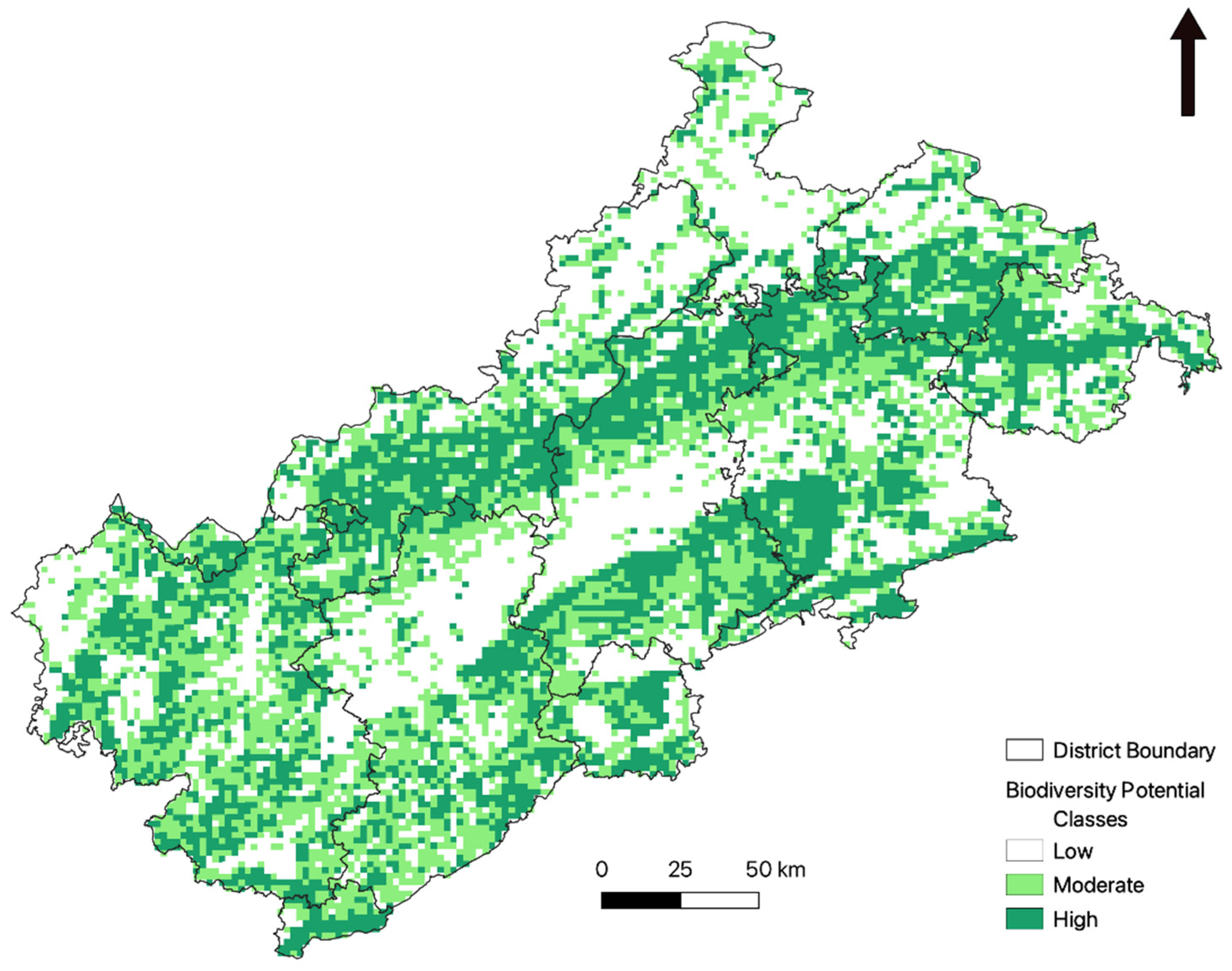
3.1. Biodiversity Potential

Biodiversity potential scores ranged from 0.086 to 0.535 for 12,492 grids of size 4 km2 (including small partially clipped grids at the edge of landscape boundary) (Figure 2). The low biodiversity potential class had 4674 (37.41%) grids (2 km × 2 km), the moderate biodiversity potential class had 3931 (31.46%) grids, and the high biodiversity potential class had 3887 grids (38.11%) (Figure 2). Most of the low biodiversity potential PUs were in the agriculture areas, and high biodiversity potential PUs were in forest areas.
A total of 32 species of mammal and 355 species of vegetation were recorded during field sampling. Field measured species richness for different taxa was found to increase with the increase in biodiversity potential, except for herbivores, primates, and rodents, which have fewer species and are also present throughout the landscape. Kruskal–Wallis test using all taxa (data in Table 3) showed no statistically significant difference (chi-squared = 2.538, df = 2, p = 0.281, 95% confidence interval) between the three biodiversity potential classes. However, a statistically significant difference (chi-squared=7.758, df = 2, p-value = 0.021) was noted if the species richness for herbivores, primates, and rodents was removed.
The multinomial logistic regression and z-test found all of the variables to be statistically significant except for rodent richness in the moderate biodiversity potential category (Supplementary Information, Table S3). The overall classification accuracy in predicting the biodiversity potential classes using field species richness data was 65.1%. It was observed that most of the misclassifications were between the moderate and high biodiversity potential classes and together represented 93.37%, reflecting that the surrogate approach to define biodiversity potentials has empirical support to classify the area of low with the rest of the classes.

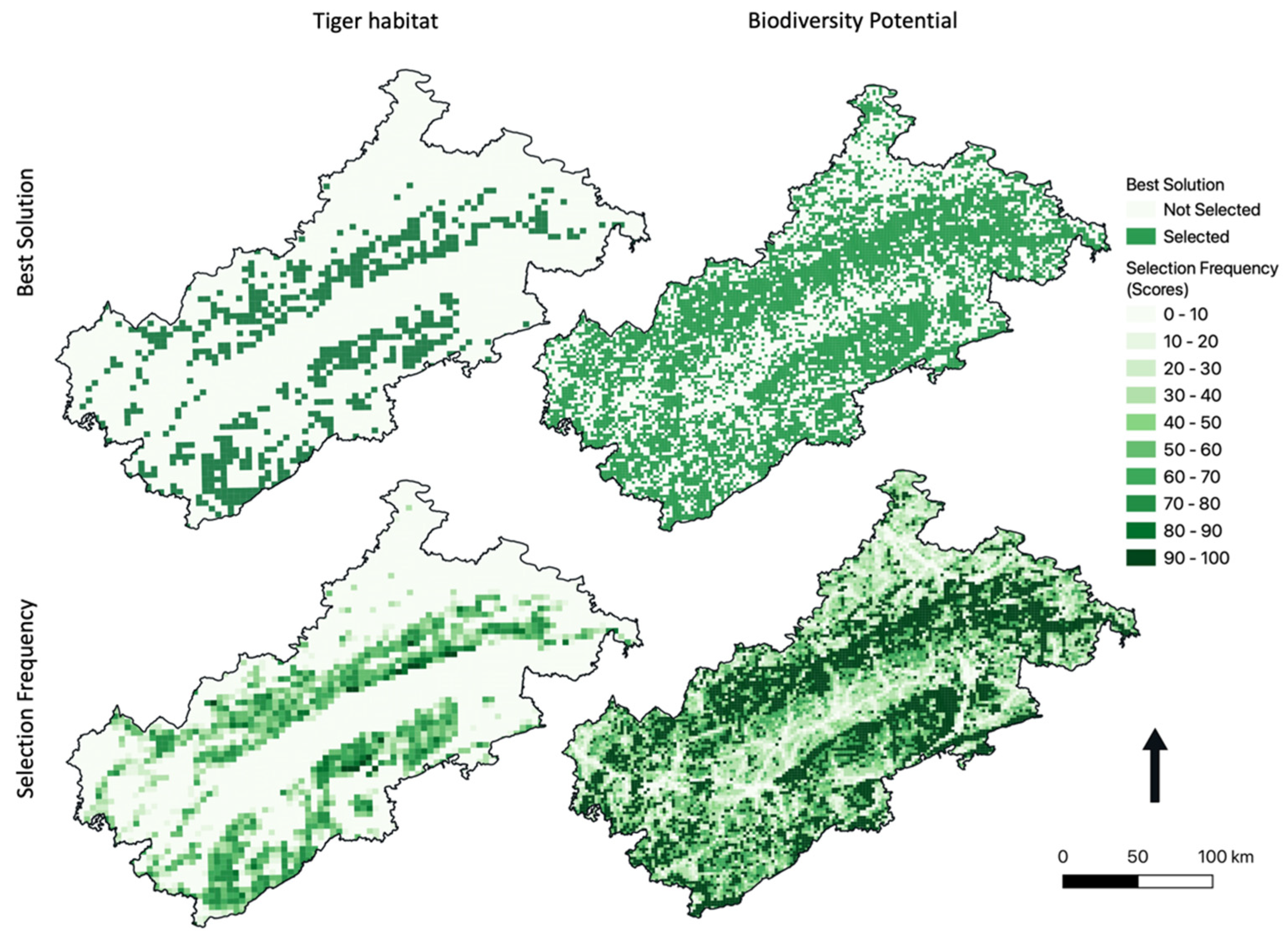
3.2. Prioritization for Tiger Habitat and Biodiversity Potential

For tiger habitat, 610 (18.85%) PUs out of 3236 available PUs were selected in the best solution (Table 4, Figure 3). This constitutes 9345.03 km2 area (18.87% of the landscape). For biodiversity potential, overall, 6963 (55.73%) PUs out of available 12,492 units were selected (Table 4, Figure 3). This constitutes an area of 27,315.09 skm2 (55.15% area of the landscape). Further within biodiversity potential, 1122 PUs were selected with low biodiversity potential, 1954 PUs with moderate biodiversity potential, and 3887 PUs with high biodiversity potential (Table 4). An area of 4201.15 km2 (8.48% of the landscape area) was selected with low biodiversity potential, 7702.19 km2 (15.55% of the landscape area) of moderate, and 15,411.75 km2 (31.12% of the landscape area) of the area falls within the existing protected areas. As a whole, this configuration would conserve 29,260.12 km2 area (59.08% of the geographical area of the GPL).

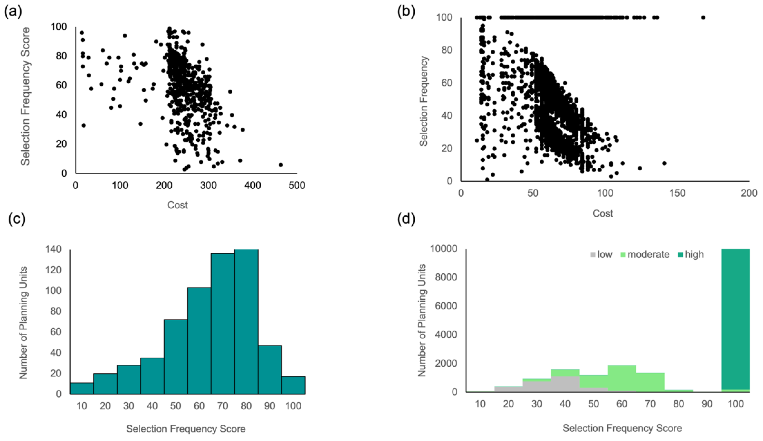
3.3. Cost and Selection Frequency

In terms of the cost of planning units for tiger habitat, the majority of planning units were selected within a narrow range of 200 to 400 (Figure 4a), while for biodiversity potential, we observed selection of PUs with a cost greater than 50 and a decline in SF scores with increasing cost (Figure 4b). In terms of tiger habitat, the selection frequency scores of the selected PUs spanned over the entire range of classes, i.e., from 0–10 to 90–100 (Figure 4c). The majority of PUs had an SF score between 70 and 80, which means that they were selected in the best solution in 70 to 80 runs out of 100 runs. For biodiversity potential, the target for high biodiversity was met in the top decile of SF scores with a total of 3887 PUs (Figure 4d). For moderate biodiversity potential, the target was achieved at the fifth decile of SF scores (50–60). For low biodiversity potential, the target was met in the seventh decile of SF scores (30–40). Therefore, the selection of PUs having SF scores greater than 50 will only achieve targets for high and moderate biodiversity potential.

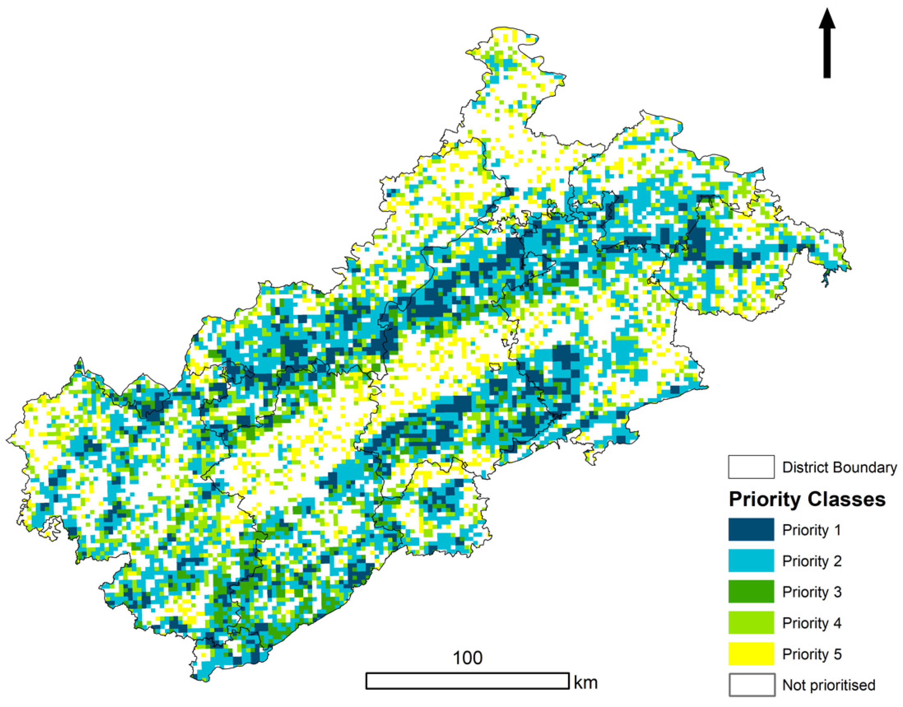
3.4. Priority Areas for Conservation

We obtained eight unique combinations of priorities with tiger and biodiversity potential—namely, (1) tiger only, (2) tiger and high biodiversity potential, (3) tiger and moderate biodiversity potential, (4) tiger and low biodiversity potential, (5) only high biodiversity potential, (6) only moderate biodiversity potential, (7) only low biodiversity potential, and (8) not selected for tiger or biodiversity potential. We merged these eight categories to obtain six categories as (1) priority I (tiger and high biodiversity potential); (2) priority II (tiger and moderate biodiversity potential; only high biodiversity potential); (3) priority III (only tiger; tiger and low biodiversity potential); (4) priority IV (only moderate biodiversity potential); (5) priority V (only low biodiversity potential), and (6) not prioritized (Figure 5). We further recommended management actions for these zones ranging from strict protection to community-based conservation and restoration (Table 5).
District Panna held the maximum area under priority I, followed by Chhatarpur, Sagar, and others (Table 6). Sagar held the maximum area under priority II, followed by Satna, Chhatarpur, and others. Damoh held the maximum area under priority III, followed by Sagar, Panna, and others. Sagar held the maximum area under priority IV, followed by Chhatarpur, Damoh, and others. Panna held the maximum area under priority V, followed by Sagar, Damoh, and others. District Sagar also held the maximum area under the non-prioritized category.

4. Discussion

4.1. Accounting for Biodiversity

We undertook a biodiversity-centric approach by integrating biodiversity potential into the tiger conservation framework at the landscape scale, taking human footprint as a constraint. As species distribution and abundance status were available for a few protected areas and fewer taxa in the landscape [79], we opted for a coarse filter approach [80,81,82], and therefore, we set targets for land cover type and a surrogate measure for biodiversity potential. An advantage of this method is that the species or taxa bias can be avoided [82], and it is more representative encompassing various habitat features and taxa than covered by fewer protected areas. Additionally, incorporating connectivity in the prioritization of tiger habitat allowed the inclusion of ecological processes (e.g., dispersal) instead of purely structural habitat information.
Biodiversity is a complex encapsulation of the structure, function, distribution, traits, and composition of all living things at different scales, and measuring and monitoring biodiversity are equally complex [83]. Methodological frameworks used for landscape-level characterization of biodiversity have a similar hypothesisthat biological richness is a function of variables such as disturbance, biogeographical setting of the landscape, structural habitat, and terrain complexity [84,85,86]. In recent decades, remote sensing techniques have been used widely to acquire synoptic data that are explicit and can be collected at multiple spatiotemporal scales [38,84,85,86]. Environmental variables and indicators derived from remotely sensed imagery can provide distinct information specific to biodiversity and its richness [87]. Satellite-derived biodiversity indicators such as topography, land cover, and vegetation (vegetation productivity) have been used in the last few decades to assess biodiversity [88,89,90,91,92]. These studies confirmed that these indicators were efficient in predicting the species richness in different habitat types with high accuracies (sometimes >90%). Duro et al. [93] recommended four broad categories of key indicators—namely, topography, land cover, vegetation (vegetation productivity), and disturbance for national biodiversity monitoring in Canada, based solely on remote sensing datasets.
In our study, we used ecological, biophysical, and anthropogenic variables to account for habitat variability and, therefore, representation of most taxa in the landscape, which is similar to other studies mentioned above. A notable difference, however, was that we chose to use field-measured species richness for testing representation of the biodiversity potential classes, rather than using species richness data as input to compute the biodiversity potential. The primary reason was that we wanted to develop a simple method that can be replicated across the country using open access and freely available datasets. Nonetheless, we observed that field-measured species richness was able to explain biodiversity potential classes. The classification accuracy was 65%, which is mainly due to the fuzzy nature of these classes, and it increased to ~93% upon merging the moderate and high classes. We acknowledge that biotic and abiotic conditions are subject to change with time, and the availability of new or better data in the future can improve decision making. In such situations, this framework can be adapted to include the new information. Therefore, this index is intended to be used as an indicator and not an absolute measure of biodiversity.

4.2. Landscape and Jurisdictional Approaches

The integrated landscape approach (or landscape approach) to conservation and development is a long-term engagement that attempts to achieve the balance between multiple goals, involving diverse stakeholders that address conflicts in land use [94]. It extends beyond traditional management practices and addresses the complex social, political, and environmental challenges associated with sustainable use of land [95]. For example, integrated landscape approaches have been used in Indonesia to achieve sustainability and conservation goals [96]. Similarly, jurisdictional approaches define landscape by policy-relevant boundaries and apply policies and practices at these jurisdictional scales to halt deforestation and degradation [97,98]. Jurisdictional approaches offer both advantages and challenges in implementing landscapes, but their success or failure is yet to be observed, as they are comparatively newer [97]. Nonetheless, jurisdictional approaches are relevant in the case of countries where decision making occurs at multiple levels, for example, in India, Ghana, etc. [97,99]. On the other hand, the landscape approach has been widely advocated despite the lack of empirical data that would prove its effectiveness [94]. Similarly, a study by McIntosh et al. [100] highlighted that the literature on systematic conservation planning is dominated by methodological studies, with fewer examples of implementation and outcomes.
The approach used in our study allows a mix of both landscape and jurisdictional approaches, with context-specific implementation targeted for each district. Further, the systematic conservation planning framework offers an objective method that can be repeated for each district at finer scales keeping the “big picture” of landscape targets as a guiding post. With the area under each priority level highlighted for each district in the landscape, fine-scale data at the district level can be used to create district-level plans. This can involve local communities in decision making and address specific issues at the local scale. For example, local knowledge on biodiversity can guide the designation of community reserves and the selection of tree species for plantation under compensatory afforestation (CAMPA) and agroforestry initiatives. Similarly, for eco-tourism and nature-based livelihood options, several local factors such as education and socioeconomics can be taken into consideration.

4.3. Policy vs. Evidence-Based Targets for Conservation

Setting clear goals and objectives is an integral part of the framework of systematic conservation planning and prioritization [101]. This is achieved by setting targets that allow the progress to be measured against a benchmark [67]. However, tools such as Marxan cannot answer questions related to the extent to which a site should be protected, and what proportion of a feature or species must be conserved. In the history of conservation planning, targets have been found to range from policy-driven to evidence-based where policy-driven targets have little to no scientific grounding, and evidence-based targets are based on measures such as habitat suitability of the species or area requirement for the population viability [102]. Targets that address representation, resiliency, and redundancy add much-needed biological grounding to somewhat “arbitrary” policy-driven and analytical targets [103,104]. Large carnivores bring an important perspective to the conservation targets by playing the role of umbrella species [105]. For the current land-use change, they have been found to work as surrogates for several other threatened species of birds, amphibians, mammals, and reptiles [106]. However, a 17% target will not be sufficient to represent all the carnivores equally and will require a target of 21% and 24% for the current and future land-use change scenario, respectively [107]. Therefore, by setting targets of 50% for tiger habitat, we were able to avoid the arbitrariness of the targets.

4.4. What Will Priority Levels Mean for Protection and Conservation?

Based on the priority level, we suggest management or conservation actions be implemented for each priority level. Priority I areas that are important for both tiger and biodiversity can be declared inviolate areas, with the least human disturbance. These areas must then be non-negotiable for any proposed development project, as they interfere with tiger dispersal and future natural colonization. Priority II area will require enhanced protection since this is contiguous with priority I area. The protection can be offered by the local communities living in the vicinity with support from the forest department. Priority III area holds significance for tigers but has low biodiversity potential. Therefore, these sites can be targeted for restoration based on local population estimates. Priority IV area holds moderate biodiversity potential and, therefore, must focus on protection and restoration activities. Priority V area largely coincides with the agricultural areas and has low biodiversity potential. Private land conservation area approaches [108], organic farming, or agroforestry initiatives are possible in these sites to restore ecosystem services [109,110].
The priority levels will work as blueprints for the entire landscape and will be effective only when recommended actions are implemented. For example, priority I sites will have no effect on conservation if the contiguous priority II areas are highly disturbed. Further, there will be a need for effective collaborative partnerships and mutual learning between managers of the districts and the PAs [92]. A network theory approach can be extremely useful in this context as the GPL implements its conservation strategy in the future [111]. Additionally, it must be noted that the recommended actions will look very different in agriculture dominant and forest dominant districts. There cannot be a one-size-fits-all approach within the landscape. Each district has different issues and different species composition and, therefore, requires a different stakeholder engagement process at the district and village levels. At the level of each district, integrated district management plans must be made to incorporate conservation strategies. These strategies can vary from community reserves, sacred groves, social forestry, organic farming, or private land conservation areas depending on the land use and socioeconomics. Recently, organic farming, agroforestry, and other nature-based solutions are proving crucial in conserving biodiversity and adding new evidence to achieve sustainable development and conservation goals [108,109,111]. With three-fourths of the population involved in the agriculture sector and millions of people living around protected areas, developing countries such as India require unified approaches to meet the national and global commitments made for biodiversity conservation and human well-being.

4.5. Opportunities

Setting targets for biodiversity alone is not sufficient for conservation [21]. It requires a balanced approach between ecological, social, and economic aspects of the landscape. Biodiversity conservation, especially for large carnivores, is affected by the nature of human–wildlife relationships (e.g., traditional values) and socioeconomics of the landscape [112,113,114,115]. These relationships and people’s perception toward wildlife and conservation are often driven by factors that vary with scale (e.g., at household and village level) but also across and between landscapes [112,113,116,117]. Therefore, more efforts are required to understand these relationships and integrate them into planning at the local scale [114]. Further, this analysis can benefit from the availability of detailed socioeconomic cost data and ecosystem service supply maps in the landscape, as utilized in other studies [118].

5. Conclusions

Conservation of tigers is an international priority but also a complex and challenging task [3], particularly when conservation overlaps with livelihood and development goals in the spatial context. As India is observing an increase in tiger population, we advocate the need to consider other taxa in conservation plans and adopt a more integrated approach in tiger landscapes. Acknowledging the fact that empirical data on the status of biodiversity will always be limited, the biodiversity potential index using open-source earth observation data can account for general patterns of biodiversity potential and reflect the restoration opportunities. Significantly, the field-measured species richness for representative taxa could explain the biodiversity potential across the landscape. Marxan, a decision-making tool for conservation management, allowed objectively selecting sites in a framework that can be adapted to changing landscape characteristics (e.g., land use, human population, policies) incorporating umbrella species and other biodiversity components. Given the spatially explicit outcome, stakeholder engagement for setting conservation targets can be plausible. Further, the area under each priority level in different districts of the landscape can be used for long-term land-use policy and integrated development actions. The methodological framework can be scaled up to other regions across India and used in other tiger range countries for land managers and decision makers to allocate resources that are often limited in developing countries.

Supplementary Materials

The following supporting information can be downloaded at: www.mdpi.com/xxx/s1.Table S1: Description of terms used in this study, Table S2: Resistance matrix used for calculation of connectivity with the least cost path method, Table S3: Coefficients, standard error, and p values for logistic regression and z-test, Table S4: Confusion matrix for multinomial logistic regression model, Figure S1: Distribution of field sampling points in the landscape.

Author Contributions

Methodology, data processing, formal analysis, software, and visualization, writing—original draft preparation, and writing—review and editing, V.V.; methodology, data processing, and analysis, S.U.; methodology, data collection, field coordination, and writing—review and editing, A.S., N.S., S.D., R.R. and S.C.; methodology, project coordination, and writing—review and editing, S.V.; project administration and supervision, J.A.J.; conceptualization, methodology, funding acquisition, resources, project administration, supervision, and writing—review and editing, R.K. All authors have read and agreed to the published version of the manuscript.

Funding

The study was carried out as part of the project “Development of Landscape Management Plan and Monitoring Strategy with reference to Ken–Betwa River Link Project in Panna Tiger Reserve, Madhya Pradesh”, funded by the National Water Development Agency, Government of India(No. WII/KR/PROJECT/PLMP/2017-18/F(1)).

Data Availability Statement

The data used in this study are open source and can be freely downloaded from respective sources. Other data can be accessed from the corresponding author upon reasonable request.

Acknowledgments

We acknowledge the support of the Dean and Director of Wildlife Institute of India, Madhya Pradesh Forest Department, and National Tiger Conservation Authority for the long-term study in this landscape. We are grateful to Field Director, Divisional Forest Officers, and other frontline staff in the landscape for facilitating and supporting the fieldwork. We also acknowledge the project team members and advisors for regular inputs during the project activities. We thank Amaljith AT, Avishna Arappil, Satyasarathi Mishra, Purnima Singh, Subhechha Tapaswini, Bhavika Vaghjiani, and Mamtha Nayal, for assisting in the field.

Conflicts of Interest

The authors declare that they have no conflict of interest.

References

  1. Woodley, S.; Bertzky, B.; Crawhall, N.; Dudley, N.; Londoño, J.M.; MacKinnon, K.; Redford, K.; Sandwith, T. Meeting Aichi Target 11: What does success look like for protected area systems. Parks 2012, 18, 23–36. [Google Scholar]
  2. ENVIS. Protected Areas of India. 2021. Available online: http://www.wiienvis.nic.in/Database/Protected_Area_854.aspx (accessed on 24 January 2022).
  3. Rastogi, A.; Hickey, G.M.; Badola, R.; Hussain, S.A. Saving the superstar: A review of the social factors affecting tiger conservation in India. J. Environ. 2012, 113, 328–340. [Google Scholar] [CrossRef] [PubMed]
  4. Sabu, M.M.; Pasha, S.V.; Reddy, C.S.; Singh, R.; Jaishanker, R. The effectiveness of Tiger Conservation Landscapes in decreasing deforestation in South Asia: A remote sensing-based study. Spat. Inf. Res. 2021, 30, 63–75. [Google Scholar] [CrossRef]
  5. Jhala, Y.; Gopal, R.; Mathur, V.; Ghosh, P.; Negi, H.S.; Narain, S.; Yadav, S.P.; Malik, A.; Garawad, R.; Qureshi, Q. Recovery of tigers in India: Critical introspection and potential lessons. People Nat. 2021, 3, 281–293. [Google Scholar] [CrossRef]
  6. Kumar, U.; Awasthi, N.; Qureshi, Q.; Jhala, Y. Do conservation strategies that increase tiger populations have consequences for other wild carnivores like leopards? Sci. Rep. 2019, 9, 14673. [Google Scholar] [CrossRef] [PubMed] [Green Version]
  7. Walston, J.; Stokes, E.J.; Hedges, S. The importance of Asia’s protected areas for safeguarding commercially high value species. In Protected Areas: Are They Safeguarding Biodiversity; Wiley: London, UK, 2016; pp. 190–207. [Google Scholar]
  8. Karanth, U.K. Tiger ecology and conservation in the Indian subcontinent. J. Bombay Nat. Hist. Soc. 2003, 100, 169–189. [Google Scholar]
  9. McNab, B.K. Bioenergetics and the determination of home range size. Am. Nat. 1963, 97, 133–140. [Google Scholar] [CrossRef]
  10. Noss, R.F.; Quigley, H.B.; Hornocker, M.G.; Merrill, T.; Paquet, P.C. Conservation biology and carnivore conservation in the Rocky Mountains. Conserv. Biol. 1996, 10, 949–963. [Google Scholar] [CrossRef]
  11. Seddon, P.J.; Leech, T. Conservation short cut, or long and winding road? A critique of umbrella species criteria. Oryx 2008, 42, 240–245. [Google Scholar] [CrossRef] [Green Version]
  12. Wang, F.; Winkler, J.; Vina, A.; McShea, W.J.; Li, S.; Connor, T.; Zhao, Z.; Wang, D.; Yang, H.; Tang, Y.; et al. The hidden risk of using umbrella species as conservation surrogates: A spatio-temporal approach. Biol. Conserv. 2021, 253, 108913. [Google Scholar] [CrossRef]
  13. Thornton, D.; Zeller, K.; Rondinini, C.; Boitani, L.; Crooks, K.; Burdett, C.; Rabinowitz, A.; Quigley, H. Assessing the umbrella value of a range-wide conservation network for jaguars (Panthera onca). Ecol. Appl. 2016, 26, 1112–1124. [Google Scholar] [CrossRef] [PubMed] [Green Version]
  14. Bifolchi, A.; Lodé, T. Efficiency of conservation shortcuts: An investigation with otters as umbrella species. Biol. Conserv. 2005, 126, 523–527. [Google Scholar] [CrossRef]
  15. Poiani, K.A.; Merrill, M.D.; Chapman, K.A. Identifying conservation-priority areas in a fragmented Minnesota landscape based on the umbrella species concept and selection of large patches of natural vegetation. Conserv. Biol. 2001, 15, 513–522. [Google Scholar] [CrossRef]
  16. Caro, T.M.; O’Doherty, G. On the use of surrogate species in conservation biology. Conserv. Biol. 1999, 13, 805–814. [Google Scholar] [CrossRef]
  17. Krishnamurthy, R.; Cushman, S.A.; Sarkar, M.S.; Malviya, M.; Naveen, M.; Johnson, J.A.; Sen, S. Multi-scale prediction of landscape resistance for tiger dispersal in central India. Landsc. Ecol. 2016, 31, 1355–1368. [Google Scholar] [CrossRef]
  18. Vasudev, D.; Goswami, V.R.; Srinivas, N.; Syiem, B.L.N.; Sarma, A. Identifying important connectivity areas for the wide-ranging Asian elephant across conservation landscapes of Northeast India. Divers. Distrib. 2021, 27, 2510–2526. [Google Scholar] [CrossRef]
  19. MEA (Millennium Ecosystem Assessment). Ecosystems and Human Well-Being, Volume 2, Scenarios; Island Press: Washington, DC, USA, 2005; Available online: http://www.millenniumassessment.org/en/Scenarios.aspx (accessed on 7 January 2022).
  20. Sayer, J.; Bullb, G.; Elliott, C. Mediating Forest Transitions: ‘Grand Design’ or ‘Muddling Through’. Conserv. Soc. 2008, 6, 320–327. [Google Scholar] [CrossRef]
  21. Wiens, J.A. Landscape ecology as a foundation for sustainable conservation. Landsc. Ecol. 2009, 24, 1053–1065. [Google Scholar] [CrossRef]
  22. Mascia, M.B.; Pailler, S. Protected area downgrading, downsizing, and degazettement (PADDD) and its conservation implications. Conserv. Lett. 2011, 4, 9–20. [Google Scholar] [CrossRef]
  23. Forrest, J.L.; Mascia, M.B.; Pailler, S.; Abidin, S.Z.; Araujo, M.D.; Krithivasan, R.; Riveros, J.C. Tropical deforestation and carbon emissions from protected area downgrading, downsizing, and degazettement (PADDD). Conserv. Lett. 2015, 8, 153–161. [Google Scholar] [CrossRef]
  24. Jha, K.K.; Jha, R.; Campbell, M.O.N. The distribution, nesting habits and status of threatened vulture species in protected areas of Central India. Ecol. Quest. 2021, 32, 1–27. [Google Scholar] [CrossRef]
  25. Stevenson, C.J. Conservation of the Indian Gharial Gavialis gangeticus: Successes and failures. Int. Zoo Yearb. 2015, 49, 150–161. [Google Scholar] [CrossRef]
  26. Gopal, R.; Qureshi, Q.; Bhardwaj, M.; Singh, R.J.; Jhala, Y.V. Evaluating the status of the endangered tiger Panthera tigris and its prey in Panna Tiger Reserve, Madhya Pradesh, India. Oryx 2010, 44, 383–389. [Google Scholar] [CrossRef] [Green Version]
  27. Sarkar, M.S.; Ramesh, K.; Johnson, J.A.; Sen, S.; Nigam, P.; Gupta, S.K.; Murthy, R.S.; Saha, G.K. Movement and home range characteristics of reintroduced tiger (Panthera tigris) population in Panna Tiger Reserve, central India. Eur. J. Wildl. Res. 2016, 62, 537–547. [Google Scholar] [CrossRef]
  28. Dinerstein, E.; Wikramanayake, E.D.; Robinson, J.; Karanth, U.; Rabinowitz, A.; Olson, D.; Mathew, D.; Hedao, P.; Connor, M. Part 1: A framework for identifying high priority areas for the conservation of free-ranging tigers. In A Framework for Identifying High Priority Areas and Actions for the Conservation of Tigers in the Wild; WWF: Washington, DC, USA; WCS: New York, NY, USA, 1997. [Google Scholar]
  29. Dinerstein, E.; Loucks, C.; Heydlauff, A.; Wikramanayake, E.; Bryja, G.; Forrest, J.; Ginsberg, J.; Klenzendorf, S.; Leimgruber, P.; O’Brien, T.; et al. Setting priorities for the conservation and recovery of wild tigers: 2005–2015. In Tigers of the World; A User’s Guide; World Wildlife Fund, Wildlife Conservation Society, Smithsonian Institution, and National Fish and Wildlife Foundation–Save the Tiger Fund: Washington, DC, USA, 2006. [Google Scholar]
  30. Smith, J.L.D.; Ahearn, S.C.; McDougal, C. Landscape analysis of tiger distribution and habitat quality in Nepal. Conserv. Biol. 1998, 12, 1338–1346. [Google Scholar] [CrossRef]
  31. Wikramanayake, E.; McKnight, M.; Dinerstein, E.; Joshi, A.; Gurung, B.; Smith, D. Designing a conservation landscape for tigers in human-dominated environments. Conserv. Biol. 2004, 18, 839–844. [Google Scholar] [CrossRef]
  32. Harihar, A.; Pandav, B.; MacMillan, D.C. Identifying realistic recovery targets and conservation actions for tigers in a human-dominated landscape using spatially explicit densities of wild prey and their determinants. Divers. Distrib. 2014, 20, 567–578. [Google Scholar] [CrossRef] [Green Version]
  33. Kang, D.; Yang, H.; Li, J.; Chen, Y. Can conservation of single surrogate species protect co-occurring species? Environ. Sci. Pollut. Res. 2013, 20, 6290–6296. [Google Scholar] [CrossRef]
  34. Wang, F.; McShea, W.J.; Li, S.; Wang, D. Does one size fit all? A multispecies approach to regional landscape corridor planning. Divers. Distrib. 2018, 24, 415–425. [Google Scholar] [CrossRef] [Green Version]
  35. Barlow, N.L.; Kirol, C.P.; Doherty, K.E.; Fedy, B.C. Evaluation of the umbrella species concept at fine spatial scales. J. Wildl. Manag. 2020, 84, 237–248. [Google Scholar] [CrossRef]
  36. Cohen, M.; Varga, D.; Vila, J.; Barrassaud, E. A multi-scale and multi-disciplinary approach to monitor landscape dynamics: A case study in the Catalan pre-Pyrenees (Spain). Geogr. J. 2011, 177, 79–91. [Google Scholar] [CrossRef]
  37. De Aranzabal, I.; Schmitz, M.F.; Pineda, F.D. Integrating landscape analysis and planning: A multi-scale approach for oriented management of tourist recreation. Environ. Manag. 2009, 44, 938–951. [Google Scholar] [CrossRef] [PubMed]
  38. Nagendra, H.; Gadgil, M. Biodiversity assessment at multiple scales: Linking remotely sensed data with field information. Proc. Natl. Acad. Sci. USA 1999, 96, 9154–9158. [Google Scholar] [CrossRef] [Green Version]
  39. Yu, H. A multi-scale approach to mapping conservation priorities for rural China based on landscape context. Environ. Dev. Sustain. 2020, 1–26. [Google Scholar] [CrossRef]
  40. Makwana, M.; Vasudeva, V.; Cushman, S.A.; Krishnamurthy, R. Modelling landscape permeability for dispersal and colonization opportunity of tigers (Panthera tigris) in the Greater Panna Landscape, Central India. Manuscript submitted for publication.
  41. Isotti, R.; Monacelli, M. Land management by bird community analysis: Comparison among mapping methods for the zonation of a mediterranean habitat. Isr. J. Ecol. Evol. 2019, 65, 137–146. [Google Scholar] [CrossRef]
  42. Pinto, R.; Antunes, P.; Blumentrath, S.; Brouwer, R.; Clemente, P.; Santos, R. Spatial modelling of biodiversity conservation priorities in Portugal’s Montado ecosystem using Marxan with Zones. Environ. Conserv. 2019, 46, 251–260. [Google Scholar] [CrossRef]
  43. Cudlín, O.; Pechanec, V.; Purkyt, J.; Chobot, K.; Salvati, L.; Cudlín, P. Are Valuable and Representative Natural Habitats Sufficiently Protected? Application of Marxan model in the Czech Republic. Sustainability 2020, 12, 402. [Google Scholar] [CrossRef] [Green Version]
  44. Liang, J.; Gao, X.; Zeng, G.; Hua, S.; Zhong, M.; Li, X.; Li, X. Coupling Modern Portfolio Theory and Marxan enhances the efficiency of Lesser White-fronted Goose’s (Anser erythropus) habitat conservation. Sci. Rep. 2018, 8, 214. [Google Scholar] [CrossRef] [PubMed] [Green Version]
  45. Jellinek, S. Using prioritisation tools to strategically restore vegetation communities in fragmented agricultural landscapes. Ecol. Manag. Restor. 2017, 18, 45–53. [Google Scholar] [CrossRef] [Green Version]
  46. Boykin, K.G.; Kepner, W.G.; McKerrow, A.J. Applying Biodiversity Metrics as Surrogates to a Habitat Conservation Plan. Environments 2021, 8, 69. [Google Scholar] [CrossRef]
  47. Reddy, C.S.; Jha, C.S.; Dadhwal, V.K. Earth observations based conservation prioritization in Western Ghats, India. J. Geol. Soc. India 2018, 92, 562–567. [Google Scholar] [CrossRef]
  48. Lawler, J.J.; White, D. Assessing the mechanisms behind successful surrogates for biodiversity in conservation planning. Anim. Conserv. 2008, 11, 270–280. [Google Scholar] [CrossRef]
  49. Rodrigues, A.S.; Brooks, T.M. Shortcuts for biodiversity conservation planning: The effectiveness of surrogates. Annu. Rev. Ecol. Evol. Syst. 2007, 38, 713–737. [Google Scholar] [CrossRef]
  50. Forest, F. Quest for adequate biodiversity surrogates in a time of urgency. Proc. Natl. Acad. Sci. USA 2017, 114, 12638–12640. [Google Scholar] [CrossRef] [PubMed] [Green Version]
  51. Daigle, R.M.; Metaxas, A.; Balbar, A.C.; McGowan, J.; Treml, E.A.; Kuempel, C.D.; Possingham, H.P.; Beger, M. Operationalizing ecological connectivity in spatial conservation planning with Marxan Connect. Methods Ecol. Evol. 2020, 11, 570–579. [Google Scholar] [CrossRef] [Green Version]
  52. Smith, R.J. The CLUZ plugin for QGIS: Designing conservation area systems and other ecological networks. Res. Ideas Outcomes 2019, 5, e33510. [Google Scholar] [CrossRef] [Green Version]
  53. Long, Z.; Gu, J.; Jiang, G.; Holyoak, M.; Wang, G.; Bao, H.; Liu, P.; Zhang, M.; Ma, J. Spatial conservation prioritization for the Amur tiger in Northeast China. Ecosphere 2021, 12, e03758. [Google Scholar] [CrossRef]
  54. Macdonald, D.W.; Bothwell, H.M.; Kaszta, Ż.; Ash, E.; Bolongon, G.; Burnham, D.; Can, O.E.; Campos-Arceiz, A.; Channa, P.; Clements, G.R.; et al. Multi-scale habitat modelling identifies spatial conservation priorities for mainland clouded leopards (Neofelis nebulosa). Divers. Distrib. 2019, 25, 1639–1654. [Google Scholar] [CrossRef] [Green Version]
  55. Aziz, A.; Barlow, A.C.; Greenwood, C.C.; Islam, A. Prioritizing threats to improve conservation strategy for the tiger Panthera tigris in the Sundarbans Reserve Forest of Bangladesh. Oryx 2013, 47, 510–518. [Google Scholar] [CrossRef] [Green Version]
  56. Ardron, J.A.; Possingham, H.P.; Klein, C.J. (Eds.) Marxan Good Practices Handbook; Version 2; Pacific Marine Analysis and Research Association: Victoria, BC, Canada, 2010; 165p, Available online: www.pacmara.org (accessed on 5 January 2022).
  57. Ball, I.R.; Possingham, H.P. Marxan (V1.8.2): Marine Reserve Design Using Spatially Explicit Annealing, a Manual. 2000. Available online: https://courses.washington.edu/cfr590/software/Marxan1810/marxan_manual_1_8_2.pdf (accessed on 7 January 2022).
  58. Temimi, M.; Leconte, R.; Chaouch, N.; Sukumal, P.; Khanbilvardi, R.; Brissette, F. A combination of remote sensing data and topographic attributes for the spatial and temporal monitoring of soil wetness. J. Hydrol. 2010, 388, 28–40. [Google Scholar] [CrossRef]
  59. Anderson, M.G.; Ferree, C.E. Conserving the stage: Climate change and the geophysical underpinnings of species diversity. PLoS ONE 2010, 5, e11554. [Google Scholar] [CrossRef] [PubMed]
  60. Latifovic, R.; Olthof, I.; Pouliot, D.; Beaubien, J. Land Cover map of Canada 2005 at 250 m Spatial Resolution. Natural Resources Canada, Earth Sciences Sector Program, and Canada Centre for Remote Sensing, Ottawa, Ontario. 2008. Available online: http://ftp.ccrs.nrcan.gc.ca/ad/NLCCLandCover/LandcoverCanada2005_250m (accessed on 10 June 2021).
  61. Olthof, I.; Pouliot, D. Treeline vegetation composition and change in Canada’s western Subarctic from AVHRR and canopy reflectance modeling. Remote Sens. Environ. 2010, 114, 805–815. [Google Scholar] [CrossRef]
  62. Rocchini, D.; Ricotta, C.; Chiarucci, A. Using satellite imagery to assess plant species richness: The role of multispectral systems. Appl. Veg. Sci. 2007, 10, 325–331. [Google Scholar] [CrossRef]
  63. Goward, S.N.; Cruickshanks, G.D.; Hope, A.S. Observed relation between thermal emission and reflected spectral radiance of a complex vegetated landscape. Remote Sens. Environ. 1985, 18, 137146. [Google Scholar] [CrossRef]
  64. Coops, N.C.; Wulder, M.A.; Duro, D.C.; Han, T.; Berry, S. The development of a Canadian dynamic habitat index using multi-temporal satellite estimates of canopy light absorbance. Ecol. Indic. 2008, 8, 754–766. [Google Scholar] [CrossRef]
  65. Wildlife Conservation Society—WCS; Center for International Earth Science Information Network—CIESIN—Columbia University. Last of the Wild Project, Version 2, 2005 (LWP-2): Global Human Footprint Dataset (Geographic); NASA Socioeconomic Data and Applications Center (SEDAC): Palisades, NY, USA, 2005. [Google Scholar] [CrossRef]
  66. Kuuluvainen, T. Disturbance dynamics in boreal forests: Defining the ecological basis of restoration and management of biodiversity. Silva Fenn. 2002, 36, 5–11. [Google Scholar] [CrossRef]
  67. Linke, S.; Pressey, R.L.; Bailey, R.C.; Norris, R.H. Management options for river conservation planning: Condition and conservation re-visited. Freshw. Biol. 2007, 52, 918–938. [Google Scholar] [CrossRef]
  68. Lehner, B.; Grill, G. Global River hydrography and network routing: Baseline data and new approaches to study the world’s large river systems. Hydrol. Process. 2013, 27, 2171–2186. [Google Scholar] [CrossRef]
  69. Qian, H.; Kissling, W.D. Spatial scale and cross-taxon congruence of terrestrial vertebrate and vascular plant species richness in China. Ecology 2010, 91, 1172–1183. [Google Scholar] [CrossRef]
  70. Castagneyrol, B.; Jactel, H. Unraveling plant–animal diversity relationships: A meta-regression analysis. Ecology 2012, 93, 2115–2124. [Google Scholar] [CrossRef]
  71. Barton, P.S.; Westgate, M.J.; Lane, P.W.; MacGregor, C.; Lindenmayer, D.B. Robustness of habitat-based surrogates of animal diversity: A multitaxa comparison over time. J. Appl. Ecol. 2014, 51, 1434–1443. [Google Scholar] [CrossRef] [Green Version]
  72. Wu, J.; Li, H.; Wan, H.; Wang, Y.; Sun, C.; Zhou, H. Analyzing the Relationship between Animal Diversity and the Remote Sensing Vegetation Parameters: The Case of Xinjiang, China. Sustainability 2021, 13, 9897. [Google Scholar] [CrossRef]
  73. Jhala, Y.V.; Qureshi, Q.; Nayak, A.K. (Eds.) Status of Tigers, Copredators and Prey in India, 2020; National Tiger Conservation Authority, Government of India: New Delhi, India; Wildlife Institute of India: Dehradun, India, 2020. [Google Scholar]
  74. Lindsay, S.J.; Dietrich, B. The Forest Flora of North-West and Central INDIA: A Handbook of the Indigenous Trees and Shrubs of Those Countries; W.H. Allen & Co.: London, UK, 1874. [Google Scholar] [CrossRef] [Green Version]
  75. Krishen, P. Jungle Trees of Central India. A Field Guide for Tree Spotters; India Penguin House India Private Limited: New Delhi, India, 2014; ISBN 9780143420743. [Google Scholar]
  76. Prater, S.H. The Book of Indian Mammals; Bombay Natural History Society: Mumbai, India, 1990; ISBN 0195621697/9780195621693. [Google Scholar]
  77. Menon, V. Indian Mammals: A Field Guide; Hachette India: Gurugram, India, 2014; ISBN 9789350097601. [Google Scholar]
  78. Venables, W.N.; Ripley, B.D. Modern Applied Statistics with S, 4th ed.; Springer: New York, NY, USA, 2002; ISBN 0-387-95457-0. Available online: https://www.stats.ox.ac.uk/pub/MASS4/ (accessed on 25 January 2022).
  79. Ghosh-Harihar, M.; An, R.; Athreya, R.; Borthakur, U.; Chanchani, P.; Chetry, D.; Datta, A.; Harihar, A.; Karanth, K.K.; Mariyam, D.; et al. Protected areas and biodiversity conservation in India. Biol. Conserv. 2019, 237, 114–124. [Google Scholar] [CrossRef]
  80. Noss, R. Protected areas: How much is enough? In National Parks and Protected Areas: Their Role in Environmental Protection; Wright, R., Ed.; Blackwell Science: Cambridge, UK, 1996; pp. 91–120. [Google Scholar]
  81. Pressey, R.L.; Cowling, R.M.; Rouget, M. Formulating conservation targets for biodiversity pattern and process in the Cape Floristic Region, South Africa. Biol. Conserv. 2003, 112, 99–127. [Google Scholar] [CrossRef]
  82. Desmet, P.; Cowling, R. Using the species–area relationship to set baseline targets for conservation. Ecology 2004, 9, 11. [Google Scholar]
  83. Skidmore, A.K.; Coops, N.C.; Neinavaz, E.; Ali, A.; Schaepman, M.E.; Paganini, M.; Kissling, W.D.; Vihervaara, P.; Darvishzadesh, R.; Feihauer, H.; et al. Priority list of biodiversity metrics to observe from space. Nat. Ecol. Evol. 2021, 5, 896–906. [Google Scholar] [CrossRef]
  84. Roy, P.S.; Tomar, S. Biodiversity characterization at landscape level using geospatial modelling technique. Biol. Conserv. 2000, 95, 95–109. [Google Scholar] [CrossRef]
  85. Roy, P.S.; Padalia, H.; Chauhan, N.; Porwal, M.C.; Gupta, S.; Biswas, S.; Jagdale, R. Validation of geospatial model for biodiversity characterization at landscape level—A study in Andaman & Nicobar Islands, India. Ecol. Modell. 2005, 185, 349–369. [Google Scholar]
  86. Roy, P.S.; Behera, M.D. Assessment of biological richness in different altitudinal zones in the Eastern Himalayas, Arunachal Pradesh, India. Curr. Sci. 2005, 88, 250–257. [Google Scholar]
  87. Wang, R.; Gamon, J.A. Remote sensing of terrestrial plant biodiversity. Remote Sens. Environ. 2019, 231, 111218. [Google Scholar] [CrossRef]
  88. Kerr, J.T.; Southwood, T.R.E.; Cihlar, J. Remotely sensed habitat diversity predicts butterfly species richness and community similarity in Canada. Proc. Natl. Acad. Sci. USA 2001, 98, 11365–11370. [Google Scholar] [CrossRef] [Green Version]
  89. Turner, W.; Spector, S.; Gardiner, N.; Fladeland, M.; Sterling, E.; Steininger, M. Remote sensing for biodiversity science and conservation. Trends Ecol. Evol. 2003, 18, 306–314. [Google Scholar] [CrossRef]
  90. Buchanan, G.M.; Nelson, A.; Mayaux, P.; Hartley, A.; Donald, P.F. Delivering a global, terrestrial, biodiversity observation system through remote sensing. Conserv. Biol. 2009, 23, 499–502. [Google Scholar] [CrossRef] [PubMed]
  91. Coops, N.C.; Wulder, M.A.; Iwanicka, D. Exploring the relative importance of satellite-derived descriptors of production, topography and land cover for predicting breeding bird species richness over Ontario, Canada. Remote Sens. Environ. 2009, 3, 668–679. [Google Scholar] [CrossRef]
  92. Rocchini, D.; Luque, S.; Pettorelli, N.; Bastin, L.; Doktor, D.; Faedi, N.; Feilhauer, H.; Féret, J.B.; Foody, G.M.; Gavish, Y.; et al. Measuring β-diversity by remote sensing: A challenge for biodiversity monitoring. Methods Ecol. Evol. 2018, 9, 1787–1798. [Google Scholar] [CrossRef] [Green Version]
  93. Duro, D.C.; Coops, N.C.; Wulder, M.A.; Han, T. Development of a large area biodiversity monitoring system driven by remote sensing. Prog. Phys. Geogr. 2007, 31, 235–260. [Google Scholar] [CrossRef]
  94. Sayer, J.A.; Margules, C.; Boedhihartono, A.K.; Sunderland, T.; Langston, J.D.; Reed, J.; Riggs, R.; Buck, L.E.; Campbell, B.M.; Kusters, K.; et al. Measuring the effectiveness of landscape approaches to conservation and development. Sustain. Sci. 2017, 12, 465–476. [Google Scholar] [CrossRef]
  95. Reed, J.; Deakin, L.; Sunderland, T. What are ‘Integrated Landscape Approaches’ and how effectively have they been implemented in the tropics: A systematic map protocol. Environ. Evid. 2015, 4, 2. [Google Scholar] [CrossRef] [Green Version]
  96. Riggs, R.A.; Achdiawan, R.; Adiwinata, A.; Boedhihartono, A.K.; Kastanya, A.; Langston, J.D.; Priyadi, H.; Ruiz-Pérez, M.; Sayer, J.; Tjiu, A. Governing the landscape: Potential and challenges of integrated approaches to landscape sustainability in Indonesia. Landsc. Ecol. 2021, 36, 2409–2426. [Google Scholar] [CrossRef]
  97. von Essen, M.; Lambin, E.F. Jurisdictional approaches to sustainable resource use. Front. Ecol. Environ. 2021, 19, 159–167. [Google Scholar] [CrossRef]
  98. Stickler, C.; Duchelle, A.E.; Nepstad, D.; Ardila, J.P. Subnational jurisdictional approaches Policy innovation and partnerships for change. In Transforming REDD+. Lessons and New Directions; Angelsen, A., Martius, C., De Sy, V., Duchelle, A.E., Larson, A.M., Pham, T.T., Eds.; CIFOR: Bogor, Indonesia, 2018; pp. 145–159. [Google Scholar]
  99. Asubonteng, K.O.; Ros-Tonen, M.A.; Baud, I.S.A.; Pfeffer, K. Envisioning the future of mosaic landscapes: Actor perceptions in a mixed cocoa/oil-palm area in Ghana. Environ. Manag. 2021, 68, 701–719. [Google Scholar] [CrossRef] [PubMed]
  100. McIntosh, E.J.; Chapman, S.; Kearney, S.G.; Williams, B.; Althor, G.; Thorn, J.P.; Grenyer, R. Absence of evidence for the conservation outcomes of systematic conservation planning around the globe: A systematic map. Environ. Evid. 2018, 7, 1–23. [Google Scholar] [CrossRef] [Green Version]
  101. Tear, T.H.; Kareiva, P.; Angermeier, P.L.; Comer, P.; Czech, B.; Kautz, R.; Landon, L.; Mehlman, D.; Murphy, K.; Ruckelshaus, M.; et al. How much is enough? The recurrent problem of setting measurable objectives in conservation. Bioscience 2005, 55, 835–849. [Google Scholar] [CrossRef] [Green Version]
  102. Svancara, L.K.; Brannon, J.R.; Scott, M.; Groves, C.R.; Noss, R.F.; Pressey, R.L. Policy-driven versus evidence-based conservation: A review of political targets and biological needs. Bioscience 2005, 55, 989–995. [Google Scholar] [CrossRef]
  103. Shaffer, M.L.; Stein, B.A. Safeguarding our precious heritage. In Precious Heritage: The Status of Biodiversity in the United States; Stein, B.A., Kutner, L.S., Adams, J.S., Eds.; Oxford University Press: New York, NY, USA, 2001; pp. 301–321. [Google Scholar]
  104. Groves, C.R. What to conserve? Selecting conservation targets. In Drafting a Conservation Blueprint: A Practitioner’s Guide to Planning for Biodiversity; Island Press: Washington, DC, USA, 2003. [Google Scholar]
  105. Barua, M. Mobilizing metaphors: The popular use of keystone, flagship and umbrella species concepts. Biodivers. Conserv. 2011, 20, 1427–1440. [Google Scholar] [CrossRef]
  106. Di Minin, E.; Slotow, R.; Hunter, L.T.; Pouzols, F.M.; Toivonen, T.; Verburg, P.H.; Leader-Williams, N.; Petracca, L.; Moilanen, A. Global priorities for national carnivore conservation under land use change. Sci. Rep. 2016, 6, 1–9. [Google Scholar] [CrossRef] [Green Version]
  107. Shumba, T.; De Vos, A.; Biggs, R.; Esler, K.J.; Ament, J.M.; Clements, H.S. Effectiveness of private land conservation areas in maintaining natural land cover and biodiversity intactness. Glob. Ecol. Conserv. 2020, 22, e00935. [Google Scholar] [CrossRef]
  108. Puri, M.; Pienaar, E.F.; Karanth, K.K.; Loiselle, B.A. Food for thought—Examining farmers’ willingness to engage in conservation stewardship around a protected area in central India. Ecol. Soc. 2021, 26, 46. [Google Scholar] [CrossRef]
  109. Maheshwari, A.; Kumar, S.; Singh, K. Natural Regeneration and Farmland Afforestation as Refugia to Biodiversity: A Case Study from Bundelkhand Region in India. Ecol. Restor. 2020, 38, 223–227. Available online: https://www.muse.jhu.edu/article/783055 (accessed on 5 February 2022). [CrossRef]
  110. Rozylowicz, L.; Nita, A.; Manolache, S.; Popescu, V.D.; Hartel, T. Navigating protected areas networks for improving diffusion of conservation practices. J. Environ. 2019, 230, 413–421. [Google Scholar] [CrossRef]
  111. Keerthika, A.; Parthiban, K.T. Multifunctional agroforestry landscapes: Augmenting butterfly biodiversity at foot hills of Nilgiris, India. Int. J. Trop. Insect Sci. 2021, 42, 545–556. [Google Scholar] [CrossRef]
  112. Vasudeva, V.; Ramasamy, P.; Pal, R.S.; Behera, G.; Karat, P.R.; Krishnamurthy, R. Factors Influencing People’s Response Toward Tiger Translocation in Satkosia Tiger Reserve, Eastern India. Front. Conserv. Sci. 2021, 2, 664897. [Google Scholar] [CrossRef]
  113. Malviya, M.; Kalyanasundaram, S.; Krishnamurthy, R. Paradox of success-mediated conflicts: Analyzing attitudes of local communities towards successfully reintroduced tigers in India. Front. Conserv. Sci. 2022, 2, 783467. [Google Scholar] [CrossRef]
  114. Blicharska, M.; Orlikowska, E.H.; Roberge, J.M.; Grodzinska-Jurczak, M. Contribution of social science to large scale biodiversity conservation: A review of research about the Natura 2000 network. Biol. Conserv. 2016, 199, 110–122. [Google Scholar] [CrossRef]
  115. Venkataraman, A. Incorporating traditional coexistence propensities into management of wildlife habitats in India. Curr. Sci. 2000, 79, 1531–1535. [Google Scholar]
  116. Nagendra, H.; Rocchini, D.; Ghate, R. Beyond parks as monoliths: Spatially differentiating park-people relationships in the Tadoba Andhari Tiger Reserve in India. Biol. Conserv. 2010, 143, 2900–2908. [Google Scholar] [CrossRef]
  117. Kolipaka, S.S.; Persoon, G.A.; De Iongh, H.H.; Srivastava, D.P. The influence of people’s practices and beliefs on conservation: A case study on human-carnivore relationships from the multiple use buffer zone of the Panna Tiger Reserve, India. Hum. Ecol. 2015, 52, 192–207. [Google Scholar] [CrossRef] [Green Version]
  118. Hemati, T.; Pourebrahim, S.; Monavari, M.; Baghvand, A. Species-specific nature conservation prioritization (a combination of MaxEnt, Co $ ting Nature and DINAMICA EGO modeling approaches). Ecol. Model. 2020, 429, 109093. [Google Scholar] [CrossRef]
Figure 1. Location and extent of Greater Panna Landscape (A) in India, (B) districts (administrative units) of Madhya Pradesh and Uttar Pradesh that are part of Greater Panna Landscape. The main map shows major land cover classes (Forest Survey of India, 2014) and protected areas in the landscape. WLS indicates Wildlife Sanctuary.
Land 11 00371 g001
Figure 2. Spatial distribution of biodiversity potential classes in Panna Landscape.
Land 11 00371 g002
Figure 3. Marxan solution as best solution and selection frequency scores for tiger habitat and biodiversity potential.
Land 11 00371 g003
Figure 4. Distribution of planning units among different selection frequency scores for (a) tiger habitat and (b) biodiversity potential. Selection frequency versus the cost of planning units for (c) tiger habitat and (d) biodiversity potential.
Land 11 00371 g004
Figure 5. Priority areas for conservation in Panna Landscape.
Land 11 00371 g005
Table 1. Earth observation data products used in the computation of variables for biodiversity potential.
Data Layers
(Data Type)
Spatial ResolutionSourceRationaleReferences
Elevation
(Continuous)
30 mASTERTopography influences regional biodiversity by generating environmental gradients and determining the pattern of vegetation productivity and species distributions. It helps in the identification of plateaus, cliffs, and gorges. [58,59]
Forest Cover 2015
(Categorical)
24 mForest Survey of IndiaLand cover maps provide direct and indirect indices of biodiversity and can differentiate broad plant communities.[47,60,61]
Land Use/Land Cover Data 2015–16
(Categorical)
54 mNRSC, ISRO
NDVI–Annual Mean 2015
(Continuous)
30 mLandsat-8 OLIVegetation productivity is directly linked to biodiversity and can identify the regional hotspots of biodiversity. Areas with high productivity have a greater concentration of species and higher species diversity, compared with areas with low productivity. [62,63,64]
Human Footprint 2012
(Continuous)
1 kmLast of the Wild [65]Disturbances from natural and human factors alter the landscape structure and functioning of ecosystems, which, in turn, impacts biodiversity and species distributions. [66,67]
NDWI- Annual Mean 2015
(Continuous)
30 mLandsat-8 OLINDWI highlights the surface water bodies, which represent the terrestrial aquatic habitats at the landscape scale.Study specific
River Drainage
(Vector Line)
-Hydrosheds [68]The drainage network accounts for gaps in the NDWI data, especially in the case of smaller streams and dry riverbeds.Study specific
Table 2. Rank and weight score assigned to the variables used in the computation of biodiversity potential.
Indicators Normalization
(0–1)
Rank AssignedWeight Score
Elevation (standard deviation)Low to High60.04
Slope (diversity)Low to High10.14
NDVI (mean)Low to High20.12
NDVI (standard deviation)Low to High20.12
NDWI (mean)Low to High50.06
NDWI (standard deviation)Low to High50.06
Land use land cover (diversity)Low to High30.10
Stream lengthLow to High70.02
Stream diversityLow to High50.06
Human footprint (mean)High to Low (1–0)40.08
Human footprint (standard deviation)High to Low (1–0)40.08
Patch density (mean)Low to High to Low30.10
Table 3. Field measured species richness in biodiversity potential classes.
Field Measured Species RichnessBiodiversity Potential
LowModerateHigh
Trees135979
Shrubs72028
Herbs675113
Carnivores131718
Herbivores899
Primates222
Rodents333
Table 4. Planning units selected for prioritization for each conservation feature.
Tiger HabitatBiodiversity Potential
OverallLowModerateHigh
Total Pus *323612492467439313887
PUs in best solution *610 6963112219543887
Area in best solution (km2)9345.0327,315.094201.157702.1915,411.75
* It includes clipped grid cells /PUs at the edge of the landscape.
Table 5. Priority levels and recommended action for different zones based on biodiversity potential and tiger habitat.
Priority LevelDescriptionRecommended Action
Priority IPrioritized for Tiger AND high biodiversity potentialInviolate and no-go areas
Priority IIPrioritized for Tiger AND moderate biodiversity potential OR only high biodiversity potentialProtection measures
Priority IIIPrioritized for Tiger AND low biodiversity potential OR prioritized only for tigerProtection measures and population augmentation for different taxa
Priority IVPrioritized only for moderate biodiversity potentialProtection, population augmentation for different taxa, and restoration
Priority VPrioritized only for low biodiversity potential Social forestry and Restoration
Table 6. District-wise area (in km2) distribution for different priority regions of conservation.
DistrictPriority IPriority IIPriority IIIPriority IVPriority VNot Prioritized
Banda19.613346.4630.638243.858411.0782010.290
Chhatarpur694.2611799.758258.014786.011657.1402243.568
Chitrakoot180.0341008.22117.365398.756219.0701247.074
Damoh531.4141617.270760.210776.400558.1922777.839
Katni127.875484.47382.768148.514170.046587.091
Lalitpur79.757119.89351.14648.1602.37355.605
Narsinghpur90.846218.97237.65237.3135.331102.288
Panna1325.4391770.633490.718569.252633.7762018.931
Rewa261.602869.60651.371394.478271.7661119.092
Sagar729.0602467.751503.4961451.900592.0633423.288
Satna673.9652169.288202.842672.608452.9272491.929
Publisher’s Note: MDPI stays neutral with regard to jurisdictional claims in published maps and institutional affiliations.

