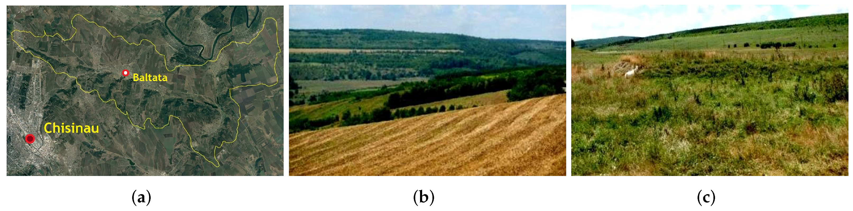
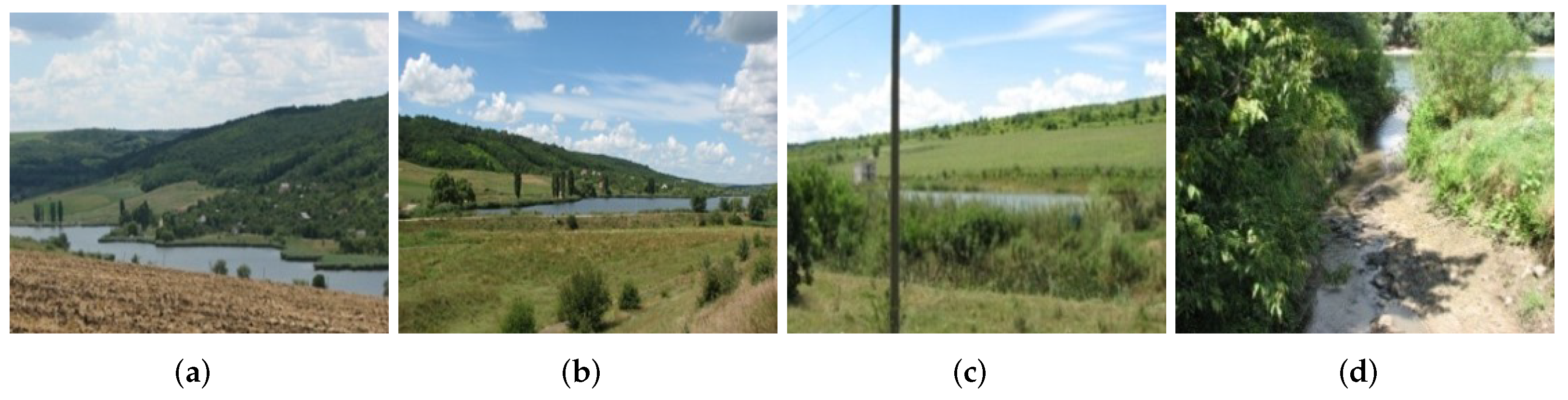
Article

Modelling Runoff within a Small River Basin under the Changing Climate: A Case Study of Using SWAT in the Bălțata River Basin (The Republic of Moldova)

1
Faculty of Natural and Agricultural Sciences, Department of Natural Sciences, Ovidius University of Constanța, 900470 Constanta, Romania
2
Eco-TIRAS International Association of River Keepers, MD-2012 Chișinău, Moldova
3
Institute of Ecology and Geography, MD-2028 Chișinău, Moldova
*
Author to whom correspondence should be addressed.
Land 2022, 11(2), 167; https://doi.org/10.3390/land11020167
Submission received: 15 December 2021 / Revised: 17 January 2022 / Accepted: 19 January 2022 / Published: 21 January 2022

Abstract

:
The article focuses on modelling surface runoff in a small river basin taking into consideration climate change projections. The runoff was modelled using the Soil and Water Assessment Tool (SWAT), while three Representative Concentration Pathways (RCP2.6, RCP4.5, and RCP8.5) were considered for modelling the future climate. Despite the identified uncertainties, all the scenarios pointed towards decreasing runoff and losing available water resources. The expected runoff of the case study basin (Bălțata River in the Republic of Moldova) will decrease under all considered scenarios. The risk of diminishing runoff will be low in the middle-term perspective and moderate in the long-term one, if considered from the yearly changes. However, there are months with a high risk of diminishing runoff, especially important for proper crop production. While in the middle-term perspective, traditional adaptation measures can be used, in the long-term one, a totally new approach should be sought.

1. Introduction

The movement and storage of water at watershed scales is a complex process affected by geologic, geomorphological, climatic, soil, land use, man-made, and other factors. The nature of the processes inherent in surface and subsurface hydrology is best investigated by hydrologic models simulating these processes over different spatial and time intervals and different physiographical conditions.
By definition, any hydrologic model is a certain simplification of a real-world water system (surface and soil waters, wetland, groundwater, estuary, etc.); such simplification aids in understanding, predicting, and managing water resources. In recent years, several conceptual hydrological simulation models have been developed and increasingly used by hydrologists and water resource managers to understand and address the extensive array of water resource problems, including those related to the watershed, streamflow, and reservoir management, as well as to human activities that affect water systems. Numerous review studies that provide comparisons of either specific components or complete hydrologic modelling packages, with varying levels of input/output data and their structure complexity, have been performed by different authors (e.g., [1,2,3,4,5,6]).
However, while hydrology as a science has a long history, V. Singh [7] attributed the birth of hydrologic modelling to the second half of the 1850s when a method for computing the time of water peak discharge was developed. Then, for over a century (until the 1960s), many ground-breaking advances were made in modelling the different components of a hydrologic cycle. These advances were based mainly on mathematical physics and laboratory or field experiments. Tracing the further evolution of hydrological modelling, the cited author emphasised the post-1960s decades when, due to the computer revolution, hydrologic modelling took a giant leap forward. Computers provided the power for performing calculations that were not available before, and as a result, a new branch of hydrology, called digital or numerical hydrology, was born. Another result was statistical or stochastic hydrology, which also requires analysing large volumes of data.
Summarizing his review of the hydrological modelling history, V. Singh [7] highlighted its several major advances and opportunities where, from the viewpoint of small river basin research, the following are of especial interest:
  • Simulation of the entire hydrology;
  • Development of research techniques that form a basis for reservoirs’ management and operation, as well as river basin simulation and hydrologic models calibrating;
  • Possibilities of two- and three-dimensional modelling due to advances in numerical mathematics;
  • Simulation of different phases of liquid flow that resulted in the simulation of water flow and sediment/pollutant transport;
  • Modelling at larger spatial scales, such as a river basin, and at small temporal scales (seconds and minutes);
  • Integration of hydrology with allied sciences, for example with climatology or river basin geomorphology; the coupling of hydrology with ecosystems gave rise to ecohydrology, while climate change issues become a part of the hydrologic analysis.
Finally, we are witnessing how computing power is exponentially increasing, and the maturing hydrology is expanding both in depth (vertically) and breadth (horizontally). Remote sensing approaches, such as satellite and drone remote sensing, came into being, which made it possible to acquire spatial data for large areas, and these huge quantities of raster and vector data are processed and statistically modelled in the Geographical Information Systems (GISs) environment.
The last point is especially important because many new research areas have emerged in the latest few decades. Thus, hydrological modelling under global environmental change, as a domain that has been receiving much attention in public fora, has arisen due to the increased frequency of hydrometeorological extremes and significant variability in the spatial and temporal distribution of precipitation. Sediment and pollutant transport in reservoirs, rivers, and other water bodies have culminated in a new field of sedimentation engineering and its prevention, especially since the 1970s with the establishment of the Environmental Protection Agency (EPA) [8].
Small rivers in hilly and plain areas usually depend on regional and local climatic and weather conditions. That is why they are extremely vulnerable to climate inter-annual variability and long-term change. At the same time, they represent a first-hand source of water for the inhabitants, especially for non-drinking purposes. This is the case of the Republic of Moldova, which mainly lies between two big rivers: Dniester and Prut. Only ∼1 million of its population lives close enough to these two rivers to rely on their water resources [9]; to them, we can add another ∼1.2 million people, which inhabit cities and towns outside this area and which have a more or less reliable central water supply. Finally, ∼1.7 million rural inhabitants (44% of the total population) have access just to sub-surface ground water and water resources contained in small rivers, both exposed to local climate variability and change. Thus, the projected availability of the small rivers’ water resources becomes extremely important for future crop production and land use planning [10]. It is important both in the Moldovan context and for other countries with regions depending on small rivers’ surface water resources in a similar manner, such as parts of Bulgaria, Romania, Ukraine, southern parts of European Russia, etc.
In order to address the above-mentioned challenges, as well as to benefit from the advantages of the existing models, our paper proposes to make an assessment of the changes of future water resources within a small river basin in their relationship with the changing climate’s parameters and specific characteristics of the active surface. Changes of water resources were evaluated using surface runoff figures, which is sensitive enough to climate parameters [11]. This assessment is required for searching for the future prospects of the adaptation measures to be implemented as a response to climate change. The assessment was performed for the Bălțata River Basin of the Republic of Moldova, which plays the role of a “lab” for environmental research in Moldova due to the availability of climate and hydrologic data from the stations located within the basin. At the same time, selecting the proper adaptation to climate change measures is particularly important for the basin because, as previous research has shown, it is among the most vulnerable to future climate change due to its proximity to the national capital [12].

2. Materials and Methods

2.1. Study Area

The Bălțata River is a small right tributary of the Dniester River, being entirely located on the territory of the Republic of Moldova. Most of the Bălțata River Basin is located within the Eurasian steppe zone, while its small northwestern part lies in the forest steppe zone (Figure 1). The basin is predominantly flat, with lowlands at the river’s mouth and an elevated plain in its upper reaches’ watershed. The altitude values vary from 16 m above sea level at the mouth to 219 m in the basin’s highest point. Nonetheless, the slope angles vary from sub-horizontal to steep ones (about 17°). Slope angles from 2° to 5° are the most common, while the true horizontal surfaces occupy less than 0.1% of the basin’s area. The western slope aspect is dominant (30%), while the eastern and southern ones are slightly rare (by 26% each); even more rare are the northern and northeastern slopes (18%).
The Bălțata River Basin belongs to the soil region of leached chernozems, with clear features of their differentiation in altitude. However, in general, the soil cover is complex and heterogeneous, presenting not only different chernozem subtypes, but forest and river alluvial soils as well. The light clays and heavy loams are dominant on the gentle (40% of the basin’s area) and low-gradient (more than 10%) slopes. There are also many ravines and landslides, which point at the strong manifestation of erosion processes.
Moldova, as a whole, and the study area, in particular, have a temperate continental climate, with mild winters with little snow and warm, often dry, summers. The main climate parameters of the Bălțata River Basin in the last climatic thirty years (1991–2020) are given in Table 1. Other climate parameters, calculated based on the modelling’s needs, are given in the corresponding sections of the article.
The main types of land use are cropland, forests, pastures and meadows, orchards, and built-up plots. About 46% of the land is used for crop production, which causes a large load on soils. Orchards and pastures occupy 13.8% and 11.4%, respectively. Only 17.4% of the basin’s area is covered by forests. Among the natural vegetation, the forest-steppe and purely steppe elements are present. Due to intensive farming with poorly implemented land protection measures, which people have been practising in the basin, more than 29% of the local soils are degraded.
As for the Bălțata River flow, due to an intensive anthropogenic load, it is completely transformed; its natural conditions have significantly changed. Almost all flow accumulates in four artificial ponds. As a result, the river channel has turned into a shallow watercourse, and water intake for serious practical needs can really be carried out only from these artificial reservoirs. The current state of the basin was one of the factors to choose it as a case study for the described research.

2.2. Methods

For runoff modelling, the ArcSWAT interface for SWAT2012 was used, which evolved from AVSWAT2000, which was developed for the earlier versions of ArcView [13]. This model is among the most widely known approaches used for basin-wide research and represents multiple decades of the development of its components [14]. The first version of SWAT appeared in the early 1990s (Version 94.2), being further enhanced and improved [15]. Due to its comprehensive nature, strong technical support, and open-access status, the SWAT model has proven to be highly flexible in addressing a wide range of water resource problems. Hundreds of SWAT-related papers have been presented at numerous scientific meetings and in dozens of articles published in peer-reviewed journals. A good review of SWAT’s extensive testing at different spatial scales was provided by Zhang et al. [6]; the widespread use of SWAT in comparison with several other leading models was demonstrated by Refsgaard et al. [3].
With quite a few input data, such as hydrological [15], geomorphological [16], basic soil, and land use categories [17], this model, described in detail by various authors [13,18,19], is an extremely effective tool for assessing water resource availability for a wide range of scales and environmental conditions across the globe (e.g., [20,21,22]). As such, SWAT has gained international acceptance as a robust interdisciplinary basin-scale modelling tool. Nevertheless, certain weaknesses encountered in some of the SWAT outputs clearly show that expanded testing of this model, initially developed and adapted to specific conditions of the USA, is needed. As Gassman et al. [14] noted, the SWAT users are to bear in mind that the modelling results should reasonably reflect the actual hydrologic processes.

2.2.1. SWAT Validation

The first experience of SWAT use in Moldova was in the early 2010s [23,24,25]. The findings have provided reliable evidence that SWAT is an effective tool for modelling Moldovan small rivers’ runoff, as well as for the assessment of anthropogenic load on their watershed.
Ideally, in our case, the SWAT validation should be carried out through a comparison of the Bălțata general flow field measurement with the SWAT modelling outputs. However, this procedure could not be applied basin-wide due to the measured data availability and artificial ponds built in its riverbed.
That is why, for the SWAT validation, the upper part of the Bălțata catchment was selected, namely the part of the basin upstream from the hydrological post where flow measurements were carried out (Figure 2). The length of this reach, conventionally called the Upper Bălțata, is 5.9 km, while its drainage area is about 54.5 sq.km.
Key procedures of SWAT validation included:
  • Creating SWAT databases;
  • Watershed delineation and defining the Hydrologic Response Units (HRUs);
  • Creation of a weather database;
  • Creation of a SWAT input database;
  • Running SWAT;
  • Analysis of the SWAT outputs.

2.2.2. Creation of the SWAT Database

Following the main purpose of SWAT validation, the research approach included its use to simulate monthly and annual water inflows into the Bălțata River mainstream and their subsequent comparison with the observed streamflow at the selected hydrological post. The study period included 5 y: from 1 January 2006 to 31 December 2010. This time interval was driven by the high reliability of hydrological observation in these years. The corresponding flow statistics are given in Table 2.
The climate of a watershed provides moisture and energy inputs that control the water balance and determine the relative importance of different components in a hydrological cycle [13]. Weather data to be used in a watershed simulation are imported once the HRU distribution has been defined. The loaded data are used to build. wgn files for the SWAT dataset (Figure 3).
The climate variables, required by SWAT, include daily precipitation, mean maximum and minimum temperatures, solar radiation, wind speed, and relative humidity. The model allows imputing these variables from observed data records or simulating from averaged monthly values. Because of practically no free access to daily weather information, to simulate the Bălțata watershed climatic conditions, the historical (2006–2010) monthly observations at the nearest Bălțata weather station were used (Table 3). Despite the fact that SWAT can generate the set of weather data for each sub-watershed, because of their relatively small size, the weather data were generated for the Upper Bălțata watershed as a whole. The standard deviations (Sds) of the climatic variables, which are additionally required for modelling, were calculated from observational data for the corresponding 30 y baseline climatic period (1981–2010).

2.2.3. Watershed Delineation and HRU Definition

The Upper Bălțata sub-basin delineation included identifying the river reaches and their sub-watersheds. The delineation was carried out in the ArcSWAT environment, using the 10 × 10 m Digital Elevation Model (DEM) built on the digitised and vectorised 1:25,000 topographical maps.
Reaches were defined as segments of the river course, which drain an area bigger than a threshold value that defines the minimum catchment area of upstream tributaries required to form a source of flow [13]. Proceeding from the Upper Bălțata watershed area (5450 ha), the threshold value was selected equal to 300 ha. According to this value and the level of relief roughness (elevation from 16 m to 219 m), 13 sub-basin outlets were automatically defined on each of the reaches upstream of Bălțata hydrological post (Figure 3). The reaches’ length ranged from 0.22 km to 6.52 km, with an average value of 1.8 km. The last outlet coincides with the post and thus reflects the entire drainage area of the selected sub-basin. Such coincidence was necessary to compare the simulated runoff from the catchment and the observed river water discharge at that point.
A Hydrologic Response Unit (HRU) is a small entity within the watershed, which has the same characteristics of the hydrologic soil type, land use, and slope, thus identifying their different combinations within the watershed. The benefit of HRUs is the increase in accuracy of the runoff prediction from the sub-watersheds [26]. Taking into account the relatively small areas of all delineated sub-watersheds, only one HRU was identified for each of them. In this case, 13 HRUs were received for the Upper Bălțata watershed above the corresponding hydrological post.
The basic characteristics required for the HRU identification were obtained from various sources. In particular, the European land use coding system CORINE was used to develop land use maps (Figure 4). The maps themselves were obtained by interpreting Landsat 5 satellite images, with their subsequent refinement using 1 m orthophoto images; furthermore, these materials were generalised and converted into a raster format. The land use of the Upper Bălțata River Basin is distributed as follows: residential areas (URBN)—499.4 ha; Orchards and vineyards (ORSD)—1073.5 ha; Agricultural land (AGRL)—3710.2 ha; broad-leaf Forests (FRSD)—658.2 ha; Water bodies (WATR)—6.5 ha.
Soil data were extracted by vectorisation of the available 1:50,000 soil maps. In particular, soils were classified according to the FAO’s Global Soil Reference Database [27] and grouped into four types: Chernozems (CH)—5252 ha; Fluvisols (FL)—237.2 ha; Gleysols (GL)—329.3 ha; Vertisols (VR)—129.3 ha.
Slope angles in the Upper Bălțata Sub-basin are on average 5.1°. Their 5 categories—less than 2°, 2° to 7°, 7° to 12°, 12° to 15°, and more than 15°—were used to cover all slope angle ranges, from sub-horizontal to steep ones; the first four categories cover 12%, 40%, 45%, and 3% of the sub-basin area, accordingly, while the last one represents a negligible figure, and therefore, it were merged with the previous class for modelling purposes.
Reclassification of land use, soil, and slope maps into SWAT formats (layers) allowed them to be overlapped, resulting in a new layer called Full HRU, which was added to the SWAT geographic database (Figure 4). The simulated runoff was calculated separately for each HRU, with its subsequent merging into the total runoff from the sub-basin.

2.2.4. Result of SWAT Validation

The results of the SWAT simulation for each year are shown in Table 4. It contains summarised information about each run of the model, including the corresponding statistics at the Upper Bălțata catchment level, and allows the preliminary assessment of the obtained estimates’ representativeness.
For each time step, SWAT calculates the amount of water that infiltrates into the soil and evaporates. The remaining water forms surface runoff that occurs whenever the rate of water application to the ground surface exceeds the rate of infiltration [19]. From this point of view, SURQ, LATQ, and GWQ determine the runoff from the HRU into the main channel, and the remaining parameters represent soil infiltration and evapotranspiration. The catchment averages are the weighted sum of each HRU’s contribution to the river flow and soil profile.
The analysis of the simulation results gave certain grounds to consider them as quite correct from a physical point of view. In particular, the total water inflow into the main channel on average exceeded the infiltration into the soil by about 5.2-times, and the average ratio of real evapotranspiration to precipitation was 0.24. Nevertheless, SWAT, as any other complex numerical model, contains a large number of input parameters and assumptions, which inevitably require their calibration. Typically, this process is aimed at a kind of model “fitting” to local conditions, thereby reducing its internal uncertainty. In practice, the calibration process boils down to finding the best fit between modelling results and coupled instrumental observations, which is achieved by changing certain parameters of the model [4,6,15].
In particular, to compare the real Bălțata River water discharge in 2006–2010 (Table 2) with the corresponding modelling results, the observed values were converted from m 3 /s to monthly and annual volumes of water runoff; in turn, the simulated runoff from the catchment to the main channel (water yields), initially expressed in millimetres (Table 4), was converted to m 3 by multiplying it by the watershed area. As we can see from Table 5, the discrepancies between observed and simulated runoff were too large to be negligible.
For example, if we express the observed annual runoff as a percentage of the simulated one, then it will be only about 8–9% of the latter. The monthly values showed a different, more complex picture: from a more than two-fold excess of the observed values over the modelled ones in March to 1–2% values during the low-water period (August-September). Although more powerful statistical tools for comparative analysis of the observed and simulated runoff is unacceptable in this case due to the relatively short series of observations, obviously, such discrepancies require a calibration of the model.
The corresponding calibration of the SWAT model for Moldova was carried out using another small river, the Cogilnic River [24]. We considered such a decision acceptable because this procedure was carried out in the framework of another project financed by the same European Fund (see the sections Funding and Acknowledgements) and by almost the same team of participants [23,24,25]. That calibration was based on monthly data due to the lack of access to daily observations.
The calibration parameters of the river runoff model are usually divided into two groups: (1) regulating river streamflow and (2) regulating its groundwater contribution [15]. The most popular parameter from the first group is the empirically developed runoff Curve Number (CN2), which describes the curve of a runoff volume [28]. This curve, based on the area’s hydrologic soil groups, land use and land cover types, and hydrologic conditions, is widely used as an efficient method for determining the approximate share of precipitation directly attributable to runoff in a particular area, especially for small catchments and hill slope plots.
The result of the calibration of Surface runoff contribution to streamflow (SURQ) by changing the CN2 is shown in Table 6. As one can see from this table, with a 10%, 20%, and 30% decrease in this parameter, the SURQ decreased accordingly. However, the resulting flow into the main channel (yield) did not change significantly, because other parameters increased proportionally. In other words, there was a kind of redistribution of precipitation between the runoff components. Even with a 30% decrease of the CN2, the total runoff decreased only within a 5% range. A similar situation was observed when manipulating the other two parameters— S O L _ A W C and E S C O .
The obtained results confirmed available evidence that the capabilities of such a powerful model as SWAT are rather limited when applied to small rivers, especially those that are subject to large man-made changes. Under these conditions, the model calibration was not able to objectively take into account all factors affecting river streamflow, thereby causing an inevitable bias in the estimates.
Thus, SWAT modelling evaluates only a certain hypothetical runoff forming in a watershed, which depends on its purely physical and geographical factors. Such runoff can be fully realised only in an environment that is “untouched” or not subject to anthropogenic transformation. These considerations lead to a natural assumption that hydrological modelling can be used for the objective quantitative assessment of an anthropogenic impact on small rivers’ flow through considering a difference between modelled and observed long-term runoff.

2.2.5. Data Preparation for the Entire River Basin

A significant man-made transformation of the Bălțata River flow was taken into account in this study. Thus, almost all the river’s flow is accumulated in four artificial ponds, three of which are located directly in the river bed and one situated on its right tributary, in the Bălăbănești area. As a result, the flow of the Bălțata River itself has turned into a shallow watercourse (Figure 5). Because of this feature, we assessed the current and potential runoff from the catchment area through modelling the potential surface runoff, including the volume of water entering the ponds.
The following fact speaks in favour of this approach. In recent years, most of the U.S. river basins have shown a decrease in runoff from 5% to 50%. This decrease persists for up to 3 y after the end of a drought, because it takes several years with average precipitation for lakes and reservoirs that feed them (or feed on them) to return to pre-arid levels1.
Since the sequence of modelling the runoff from the river watershed followed the same procedure as in the case of the SWAT validation, only the most basic intermediate steps are presented here. Thus, the division of the entire Bălțata River Basin, with a total area of 153.9 km 2 and selected threshold value of 300 ha, resulted in 27 sub-basins (Figure 6). The length of the reaches is from 0.22 km to 7.67 km (2.27 km on average); the average, maximum, and minimum areas of the sub-basins are 5.86, 26.19, and 0.23 km 2 , accordingly (Table 7).
The land use of the entire river basin is represented by settlements (URBN)—733.7 ha, arable land (AGRL)—10,103.1 ha, Pastures (PAST)—93.7 ha, perennial plantations (ORCD)—2067.9 ha, Forests (FRSD)—2323.5 ha, and Water-covered areas (WATR)—66.5 ha. All soils are grouped into four types: chernozems—14,834.4 ha; alluvial soils (fluvisols)—596.8 ha; chernozem-like soils (gleysols)—826.8 ha, and vertisols—391.4 ha. The slope angles were broken down by the degree of erosion hazard into five categories: less than 2°, from 2° to 7°, from 7° to 12°, from 12° to 15°, and more than 15°, occupying 34.3%, 31.9%, 16.6%, 15.8%, and 1.4% of the Bălțata River Basin area, respectively (Figure 7).
Reclassification of land use, soil, and slope angle maps into SWAT formats (layers) was allowed to overlap, resulting in a new layer called Full HRU, which was added to the SWAT geographic database.

3. Results and Discussion

3.1. The Runoff under the Current Climate

Climatic indicators of the Bălțata River Basin climate in 1981–2010 are summarised in Table 8. This period was chosen by the IPCC as the baseline thirty years for calculating the climate change expected in the 21st Century. The selected statistics included data on monthly mean maximum and minimum temperatures, including standard deviations from the mean (Sd) and monthly mean precipitation, which are the input parameters for SWAT runoff modelling. Other climate variables, required for modelling, were calculated by the weather generator, which is one of the tools of the SWAT model.
Results of the SWAT modelling of the Bălțata River Basin’s annual surface runoff in the current climate are shown in Figure 8 as its basic spatial distribution in this area. The runoff values are the weighted sum of each sub-basin to the river flow and a soil profile. As we can see, the maximum annual runoff (>324 mm) occurs in the extreme northwestern part of the basin and the minimum (<315 mm) in its southwestern part, south of Budești village. However, over a large part of the territory, the runoff falls within the range of 318–324 mm.
Multiplying the runoff per unit area (yield/mm) by the catchment area gives its total value in km 3 (Table 9). The minimum runoff is observed in winter (December-February) and April-May, while the highest values correspond to the period from July to September. The modelling or potential annual runoff in the Bălțata River Basin can reach 0.048 km 3 . However, given an undoubted bias in these estimates due to the above-discussed anthropogenic load on the watershed, these results should be considered with some caution. At the same time, they provide a certain basis for assessing other impacts on the runoff, for example the one caused by climate change.
In addition to modelling the potential total runoff from the basin’s area, its potential inflow into each of the four ponds was modelled. These artificial reservoirs accumulate water purely for the economic needs of the local population, first of all for irrigation of agricultural fields and household plots, as well as fish farming, recreation, etc. The simulated mean annual flow into these reservoirs currently equals from ∼0.0004 km 3 near the village Bălăbănești up to 0.017 km 3 near the village Cimișeni. Overall, more than 0.031 km 3 of water enters the ponds during the year, which amounts to about 65% of the basin’s total runoff (0.048 km 3 ), as shown in Table 8.

3.2. The Runoff under the Expected Future Climate

3.2.1. Development of the Future Climate Scenarios in the Bălțata River Basin

The modelling of possible changes in the Bălțata runoff was based on the projections of changes in local air temperature and precipitation. Assessing any climate change impacts requires high-resolution scenarios of this change. To this end, to improve regional climate models, within the framework of the World Climate Research Program, an international coordinated experiment, the so-called CORDEX2, has been carried out. As part of this global experiment, EURO-CORDEX3 has provided regional climate projections for Europe. This experiment focuses on both modelling the current climate and projecting its future changes, using fundamentally new scenarios developed by a specially created group of scientists [29]. The CORDEX results were at the base of the IPCC Fifth [30] and Sixth4 Assessment Reports.
These scenarios, called Representative Concentration Pathways (RCPs), in contrast to the previous climate changes scenarios, do not establish expected future Greenhouse Emissions (GHGs), but a time series of emissions and concentrations of a complete set of greenhouse gases, aerosols, and chemically active gases, including ozone, as well as land use and vegetation cover, which together could result in some specific (representative) characteristics of a radiative load on the climate system. The term “representative” means that each RCP scenario represents one of the variants of emissions and gas concentrations that lead to a specific radiative load. The term “trajectory” emphasises that not only long-term load levels are of interest, but also the time sequence of achieving this result.
In the 5th Report of the Intergovernmental Panel on Climate Change, four RCPs were selected as the basis for the climate change projections:
  • RCP 8.5—the pathway of a high radiative load, which will reach more than 8.5 W/m 2 by 2010 and will continue to grow for some time further. This scenario assumes stabilisation of emissions after 2100 and stabilisation of their concentrations only by 2250; the concentration of carbon dioxide ( C O 2 ) will be approximately seven-times higher than its pre-industrial level;
  • RCP 6.0 and RCP 4.5—two intermediate stabilisation pathways for which by 2100, the radiative load will stabilise at about 6 W/m 2 and 4–5 W/m 2 , accordingly, while the level of greenhouse gas concentration will gradually stabilise by 2150;
  • RCP 2.6—a stabilisation pathway for which the radiative load will reach a peak of about 3 W/m 2 by 2100, assuming that greenhouse gas emissions begin to decline after 2070.
In this work, the projection of an expected future climate in the Bălțata River Basin was based on an ensemble of 11 high-resolution regional climate models (12.5 km), which has never been achieved in previous climate projection simulations. These projections were kindly provided by the Climate Service Center at the Max Planck Institute for Meteorology (Hamburg, Germany) [31]. From this set, three RCPs (RCP2.6, RCP4.5, and RCP8.5) were selected, which represent respectively low, moderate, and high radiative loads. Such a choice of concentration options provides an estimate of the entire range of possible changes in the regional climate. The scenarios include projections of changes in mean monthly air temperatures and precipitation relative to the period 1971–2000 for the two time horizons of the assessment: 2021–2050 and 2071–2100.
The position of the Bălțata River Basin in the net of CORDEX nodes is shown in Figure 9.

3.2.2. Air Temperature Projections

The projections of future mean area temperatures in the study, developed according to CORDEX methodology, are shown in Table 10 and Figure 10.
The analysis of the results obtained showed:
  • In the case of the stabilisation of the radiative load (scenario RCP 2.6), the average annual air temperature will increase slightly: within 0.1 °C by the middle of the century and by 0.2 °C by its end. The largest increase is likely to occur along the pathway of the high radiative load (RCP 8.5). At the same time, if in the first half of the century, an increase in annual temperature will still be within the permissible interval of 2 °C, amounting to 1.6 °C, then by the end of the century, this “tolerance” will be exceeded twice, and the temperature rise will already be 4.4 °C. The pathway of intermediate stabilisation of the radiative load (RCP 4.5) begins to take adverse irreversible effects only by the late century, when the air temperature will rise 2.5 °C;
  • In contrast to the currently observed trends, the greatest, in absolute value, warming should be expected in winter, when it can amount, depending on the level of radiative load, from 0.5 °C to 2 °C by the middle of the century and from 0.8 °C to 5.1 °C by its end. A fairly high, albeit somewhat less, increase in average temperatures is also expected in the summer months and may amount to 1.5–1.7 °C by the 2050s and 4.8 °C in the last thirty years. In transitional seasons, the temperature rise will be slightly lower;
  • The effect of radiative load is clearly manifested when considering the annual course of changes in average temperatures (Figure 10). If in the first half of the century, the amplitude of changes in mean monthly temperatures is in the range from about −1 °C to 3 °C with small differences between moderate and high radiative load, then by the end of the century, the increase in mean monthly temperatures will already exceed 5 °C or more, with significant differences between the rates of greenhouse gas concentrations’ accumulation.
To assess the probable changes in maximum and minimum air temperatures, their statistical relationships with mean temperatures were used. The statistics of regression relationships between these variables, calculated for 1961–2010, are shown in Table 11.
As can be seen from the regression analysis results, there is a high and statistically significant relationship between mean temperatures and their minimum and maximum values. The correlation coefficient r of the maximum temperature with the mean temperature in all seasons, except for autumn, is about 0.97–0.98 for monthly values and 0.95 for yearly ones. Based on the determination coefficient R 2 , 95–96% of the interannual variability of the maximum temperature, except for autumn, can be explained by the variability of mean temperature. At the same time, the opposite conclusion is also true: equally, the variability of mean temperature is explained by the variability of the maximum temperature. The relationship between the minimum and mean temperature is somewhat lower; nevertheless, judging by the standard errors of the regression, it is quite sufficient for reliable statistical prediction of changes in these parameters. Note also the very high statistical significance and, consequently, the reliability of these dependencies, which is partially explained by the long duration of the observation series (50 y).
The results of the regression analysis can serve as a basis for the transition from mean air temperature projections to the projections of maximum and minimal temperatures, however with the assumption that the regression dependencies will remain the same in a new climate. The regression coefficients r 1 show the change in the dependent variables (in this case, the maximum or minimum temperature) when the predictor (mean temperature) changes by one degree. By adding T m a x and T m i n baseline values of 1971–2000 with their projected changes, one can have an idea of their expected values in the current century (Table 12).
A comparison of Table 9 and Table 11 shows that an expected absolute change in the maximum temperature will be slightly higher than similar changes in the mean temperature, while the change in the minimum temperature will be slightly lower. However, this kind of statistical analysis, which essentially presupposes a synchronous change in the mean, maximum, and minimum temperatures, is to a certain extent applicable only under conditions of a stationary climate that ensures that its mean values and variability remain unchanged over time. Undoubtedly, under conditions of man-made climate change, these statistical dependencies can be violated, and with the expansion of the scope of experiments based on regional models, as well as the possibilities of accessing them, these projections will be refined.

3.2.3. Projections of Future Precipitation

The “spottiness” and heterogeneity of precipitation, which is specific to the Moldavian part of the Dniester Basin, is caused by the heterogeneity of the underlying Earth surface [32]. It should be taken into account when assessing climate change impact on the local level. This consideration is especially important when assessing projections of future changes in precipitation. Analysis of Table 13, where the results of CORDEX modelling of expected precipitation changes are expressed in absolute and relative values, allows us to draw two main conclusions:
  • Changes in precipitation directly depend on the level of radiative load. In particular, by the middle of this century, given that the GHG emission concentration will be stabilised (scenario RCP 2.6), the annual precipitation sum in the Bălțata Basin will decrease by 5.1%; however, in the second half of the century, it will increase by 7%, primarily due to an increase in spring precipitation. Under the conditions of intermediate (RCP 4.5) or high radiative load (RCP 8.5), in the middle of century, the total annual precipitation is expected to be practically at the level of 1971–2000 (decrease by 1–2%), and in the late century, it will slightly increase, approximately by 5%. Thus, it can be expected that during the current century, changes in total annual precipitation will be around ±5%;
  • In the seasonal context, the greatest changes in precipitation are expected to occur in the summer period, when, under all the variants of the radiative load, they will decrease by 25–27% or more compared to their baseline equivalents. In other seasons, precipitation will slightly increase, especially at the moderate radiative load. Furthermore, a kind of precipitation shift in the warm period to an earlier date is expected. The smallest changes are expected in autumn precipitation.
The expected values of monthly precipitation for two horizons of their modelling can be directly judged from Figure 11.

3.2.4. Bălțata Basin Runoff in the Expected Future Climate

For SWAT modelling of possible changes in Bălțata River flow, we used air temperature and precipitation projections of the future regional climate that were discussed above. The expected values of monthly maximum and minimum temperatures and precipitation are given in Table 14. As in the case of assessing the current runoff, these values were assumed to be the same for the entire area under consideration; other climatic parameters, which are necessary for SWAT modelling, were computed by its weather generator.
The carried out modelling confirmed the currently generally accepted assumptions and previously obtained results for the Cogilnic River Basin [24], indicating the overall expected decrease in the runoff of small rivers. In particular, according to the current estimates (Table 15), a possible change in surface runoff from the Bălțata watershed, caused by future changes in the temperature and humidity conditions of the region, may occur, depending on the time horizon and radiative load, from a slight increase of 7–8% at moderate and strong radiative loads in the first half of the 21st Century to a decrease from about 8% to more than 25% at the end of the century. Positive trends in water dynamics due to global warming should not be a surprise, as they occur in different parts of the globe [33].
Seasonal projections unanimously show that from January to May, an increase of surface runoff is expected, which, in certain months, can exceed the baseline level by ∼1.5 times. For the projected period 2021–2050, the scenario related to RCP 2.6 shows different trends, compared to the other two, which highlight similar patterns in the runoff change, although the figures differ. Thus, in the first case (RCP 2.6), the period between January and June of 2021–2050 is the only one in which the runoff will increase, with peak values, in both absolute and relative terms, occurring in April. The other two models (RCP 4.5 and RCP 8.5) show a shorter increasing period (just from January to May), with peak values in January (in relative terms) and February (the highest change values in mm); here, we should add a second positive change, which is expected to occur in November (by about 22–23 mm, or ∼50%). The same difference is observed for the warm period: the RCP 2.6 scenario points to a stronger decrease of runoff (∼27–32%) with the highest to occur in August, while the other two show more moderate changes with the highest to occur in July. All three RCP scenarios agree that there will be a general decreasing trend, with almost no runoff in several months (such as, January, April and May) and with the only significant positive one in November.
Overall, the model output related to RCP 2.6 appears to be the severest scenario of future changes, in which yearly runoff will decrease by 10% in 2021–2050 and by more than 25% in 2071–2100. Regarding the other two scenarios, the one related to RCP 4.5 is more favourable, showing a higher increase in surface runoff (8.5%) in 2021–2050 and a lower decrease (−8.5%) in 2071–2100; the respective figures for RCP 8.5 are 7.4% and −20%, accordingly. Correspondingly, the volumes of water entering the basin’s water bodies will change (Table 16).
According to the gradation of risks from a runoff decrease proposed by the U.S. Department of Agriculture [34], the obtained values of a runoff change of less than 20% can be considered as a low risk, from 20% to 40% as moderate, and more than 40% as a high risk. Our findings show that just the scenario related to RCP 2.6 presents a moderate risk from a runoff decrease, which might occur in 2071–2100, while other scenarios show a low risk for the same period, and all three scenarios agree that there will be a low risk in 2021–2050, either positive (RCP 4.5 and RCP 8.5) or negative (RCP 2.6). Thus, the period 2021–2050 is suitable for more or less “classical” adaptation measures, such as using irrigation. However, their extensive use in the Bălțata River Basin is highly threatened by the Moldovan economic transition, which seems to be a common trend for Southeast Europe [35], regardless of the threats brought by global warming in this part of the continent. Moreover, we should carefully interpret the results, as in short- and medium-term perspectives, the direct influence of socio-economic and institutional factors is likely to have a more significant effect on land use and associated factors than natural ones [36]. The period 2071–2100 is going to be marked by a severe scarcity of available water, which would exert unprecedented pressure on crop production [37].

4. Conclusions

The undoubted novelty of our research lies in the fact that SWAT was used to simulate likely changes in river flow caused by global warming, while projections of climate change in the small river basin were based on using the latest regional scenarios of the future climate change in this century. However, the use of monthly information as SWAT modelling entry data can be considered as certain shortcomings, which produce uncertainties that cannot be avoided provided the limited daily data availability in the region. The modelling outputs, due to reported uncertainties, should be considered as some rough estimates only.
Despite the uncertainties, SWAT modelling is increasingly used in simulating hydrological processes in different watersheds; it is a time-saving approach, which can be successfully applied to the development of future scenarios of small rivers’ runoff transformation caused by climate change. As such, it can and should be recommended to a wide range of stakeholders, from purely scientific research to water managers and decision-makers.
Our research highlighted several important common trends that cannot be underestimated. For the period 2021–2050, a unanimous increase in surface runoff in January-May highlights the increase of water resources’ availability in this season. At the same time, in the summer period, when irrigation is strongly needed for proper crop production, a unanimously diminishing surface runoff is expected. Under these circumstances, an artificial redistribution of available water resources from winter/spring to summer months (including the use of the existing ponds, but not limited just to them) is strongly advised. It is quite obvious that if the period 2021–2050 is suitable for more or less “classical” adaptation measures, such as irrigation, then their extensive use is highly threatened not only by economic restrictions, which seem to be a common trend for Southeast Europe, but also by the rivers’ observed shallowing, primary small ones. The situation for 2071–2100 is much more severe. Winter/spring months are expected to have almost no runoff, while summer months would show a very strong negative trend.
The future research should reflect the observed dichotomy of our findings: (1) for the first projected period, more detailed hydrological models should be employed to assess more precisely the degree of soil erosion and sediment development, as well as the likely available water resources; (2) for the second projected period, completely new adaptation models should be sought because of scarce available water resources for keeping the ecological balance of the ecosystems and water supply for the satisfaction of social and economic needs, such as irrigation.

Author Contributions

Conceptualisation, R.C. and I.S.; methodology, R.C. and G.S.; software, G.S.; validation, G.S., R.C., I.S. and I.T.; writing—original draft preparation, R.C. and I.S.; writing—review and editing, I.S.; project administration, I.T.; funding acquisition, I.T. All authors have read and agreed to the published version of the manuscript.

Funding

The current work was realised in frames of the Joint Operational Black Sea Programme 2014–2020 and the Project BSB 963 “Protect-Streams-4-Sea”, with the financial assistance of the European Union. The content of this publication is the sole responsibility of the authors, and in no case should it be considered to reflect the views of the European Union.

Institutional Review Board Statement

Not applicable.

Data Availability Statement

Not applicable.

Acknowledgments

The authors would like to thank the anonymous Reviewers for their critical reading of the text and providing valuable comments, which helped improve and clarify earlier versions of this manuscript.

Conflicts of Interest

The authors declare no conflict of interest.

Notes

1
Cost of Increasing Droughts http://growingblue.com/case-studies/cost-of-increasing-droughts/ (accessed on 26 September 2016).
2
https://cordex.org/ (accessed on 30 November 2021).
3
http://www.euro-cordex.net/ (accessed on 30 November 2021).
4
https://www.ipcc.ch/reports/ (accessed on 30 November 2021).

References

  1. Beven, K. How to make advances in hydrological modelling. Hydrol. Res. 2019, 50, 1481–1494. [Google Scholar] [CrossRef] [Green Version]
  2. Daniel, E.B.; Camp, J.V.; LeBoeuf, E.J.; Penrod, J.R.; Dobbins, J.P.; Abkowitz, M.D. Watershed Modeling and its Applications: A State-of-the-Art Review. Open Hydrol. J. 2011, 9, 26–50. [Google Scholar] [CrossRef] [Green Version]
  3. Refsgaard, J.C.; Storm, B.; Clausen, T. Système Hydrologique Europeén (SHE): Review and perspectives after 30 years development in distributed physically-based hydrological modelling. Hydrol. Res. 2010, 41, 355–377. Available online: https://iwaponline.com/hr/article-pdf/41/5/355/371012/355.pdf (accessed on 30 November 2021). [CrossRef]
  4. van Liew, M.W.; Arnold, J.G.; Bosch, D.D. Problems and potential of autocalibrating a hydrologic model. Trans. ASAE 2005, 48, 1025–1040. [Google Scholar] [CrossRef] [Green Version]
  5. van Liew, M.W.; Veith, T.L.; Bosch, D.D.; Arnold, J.G. Suitability of SWAT for the Conservation Effects Assessment Project: Comparison on USDA Agricultural Research Service Watersheds. J. Hydrol. Eng. 2007, 12, 173–189. [Google Scholar] [CrossRef] [Green Version]
  6. Zhang, X.; Srinivasan, R.; van Liew, M. Multi-Site Calibration of the SWAT Model for Hydrologic Modeling. Trans. ASABE 2008, 5, 2039–2049. [Google Scholar] [CrossRef] [Green Version]
  7. Singh, V. Hydrologic modeling: Progress and future directions. Geosci. Lett. 2018, 5, 15. [Google Scholar] [CrossRef]
  8. EPA. Climate Adaptation and Erosion & Sedimentation. 2021. Available online: https://www.epa.gov/arc-x/climate-adaptation-and-erosion-sedimentation (accessed on 30 November 2021).
  9. Sîrodoev, I. Climate change and water resources. In Climate Change in Moldova: Socio-Economic Impact and Policy Options for Adaptation; 2009/2010 National Human Development Report; Oprunenco, A., Prohnițchi, V., Eds.; UNDP Moldova: Chisinau, Moldova, 2009. [Google Scholar]
  10. Wilson, T.S.; Van Schmidt, N.D.; Langridge, R. Land-Use Change and Future Water Demand in California’s Central Coast. Land 2020, 9, 322. [Google Scholar] [CrossRef]
  11. Chen, H.Y.; Huang, C.C.; Yeh, H.F. Quantifying the Relative Contribution of the Climate Change and Human Activity on Runoff in the Choshui River Alluvial Fan, Taiwan. Land 2021, 10, 825. [Google Scholar] [CrossRef]
  12. Corobov, R.; Sîrodoev, I.; Koeppel, S.; Denisov, N.; Sîrodoev, G. Assessment of climate change vulnerability at the local level: A case study on the Dniester River Basin (Moldova). Sci. World J. 2013, 2013, 173794. [Google Scholar] [CrossRef] [Green Version]
  13. Winchell, M.; Srinivasan, R.; Di Luzio, M.; Arnold, J. ArcSWAT Interface for SWAT2012: User’s Guide; Technical Report, Blackland Research Center—Texas Agricultural Experiment Station; Grassland, Soil and Water Research Laboratory—USDA Agricultural Research Service: Temple, TX, USA, 2013. [Google Scholar]
  14. Gassman, P.W.; Sadeghi, A.M.; Srinivasan, R. Applications of the SWAT Model Special Section: Overview and Insights. J. Environ. Qual. 2014, 43, 1–8. [Google Scholar] [CrossRef] [PubMed]
  15. Arnold, J.G.; Moriasi, D.N.; Gassman, P.W.; Abbaspour, K.C.; White, M.J.; Srinivasan, R.; Santhi, C.; Harmel, R.D.; van Griensven, A.; van Liew, M.W.; et al. SWAT: Model Use, Calibration, and Validation. Trans. ASABE 2012, 55, 1491–1508. [Google Scholar] [CrossRef]
  16. Raduca, C.; Boengiu, S.; Mititelu-Ionuș, O.; Enache, C. Correlation of the Relief Conditions, Hydrographic Network features and Human Interventions within the Blahnița River basin (Southwestern Romania). Carpathian J. Earth Environ. Sci. 2021, 16, 117–127. [Google Scholar] [CrossRef]
  17. Stavropoulos, S.; Zaimes, G.N.; Filippidis, E.; Diaconu, D.; Emmanouloudis, D. Mitigating Flash Floods with the Use of New Technologies: A Multi-criteria Decision Analysis to Map Flood Susceptibility for Zakynthos Island, Greece. J. Urban Reg. Anal. 2020, 12, 233–248. [Google Scholar] [CrossRef]
  18. Arnold, J.; Kiniry, J.; Srinivasan, R.; Williams, J.; Haney, E.; Neitsch, S. Soil and Water Assessment Tool, Input/Output File Documentation, Version 2012; Technical Report Technical Report 49; Texas Water Research Institute: College Station, TX, USA, 2012. [Google Scholar]
  19. Neitsch, S.; Arnold, J.; Kiniry, J.; Williams, J. Soil and Water Assessment Tool—Theoretical Documentation. Version 2009; Technical Report; Blackland Research Center—Texas Agricultural Experiment Station; Grassland, Soil and Water Research Laboratory—USDA Agricultural Research Service: Temple, TX, USA, 2011; 618p. [Google Scholar]
  20. Adeogun, A.G.; Sule, B.F.; Salami, A.W.; Daramola, M.O. Validation of SWAT Model for Prediction of Water Yield and Water Balance: Case Study of Upstream Catchment of Jebba Dam in Nigeria. Int. J. Civ. Environ. Eng. 2014, 8, 264–270. [Google Scholar]
  21. Kalogeropoulos, K.; Chalkias, C.; Pissias, E.; Karalis, S. Application of the SWAT model for the investigation of reservoirs creation. In Advances in the Research of Aquatic Environment: Volume 2; Lambrakis, N., Stournaras, G., Katsanou, K., Eds.; Springer: Berlin/Heidelberg, Germany, 2011; pp. 71–79. [Google Scholar] [CrossRef]
  22. White, E.D.; Easton, Z.M.; Fuka, D.R.; Collick, A.S.; McCartney, M.; Awulachew, S.B.; Steenhuis, T.S. A water Balance-Based Soil and Water Assessment Tool (SWAT) for Improved Performance in the Ethiopian Highlands; Conference Papers; International Water Management Institute: Addis-Ababa, Ethiopia, 2009; pp. 153–158. [Google Scholar]
  23. Corobov, R.; Syrodoev, G.; Trombitsky, I.; Galupa, D. SWAT Model in Moldova: The First Experience. In Proceeding of the International Conference Frontiers in Environmental and Water Management, Kavala, Greece, 19–21 March 2015; pp. 75–85. [Google Scholar]
  24. Corobov, R.M.; Syrodoev, G.N.; Trombitsky, I.D. Anthropogenic and Climate Change Contributions to Uncertainties in Hydrological Modeling of Small Rivers Watershed Runoff. Adv. Ecol. Environ. Res. 2016, 1, 14–34. [Google Scholar]
  25. Corobov, R.; Syrodoev, G.; Trombitsky, I.; Galupa, D. Anthropogenic factors as an element of uncertainty in hydrological modelling of water yield with SWAT. J. Eng. Sci. Technol. Rev. 2016, 9, 138–145. [Google Scholar] [CrossRef]
  26. Kavka, P. Spatial Delimitation of Small Headwater Catchments and Their Classification in Terms of Runoff Risks. Water 2021, 13, 3458. [Google Scholar] [CrossRef]
  27. IUSS Working Group WRB. World Reference Base for Soil Resources 2014, update 2015: International Soil Classification System for Naming Soils and Creating Legends for Soil Maps; Technical Report World Soil Resources Reports No. 106; Food and Agriculture Organization, FAO: Rome, Italy, 2015. [Google Scholar]
  28. Balazovicova, L.; Skodova, M. Vegetation and land use analysis for runoff estimation in small forested catchment: A case study of Tajovsky Brook in Slovakia. Carpathian J. Earth Environ. Sci. 2022, 17, 81–92. [Google Scholar] [CrossRef]
  29. Moss, R.; Edmonds, J.; Hibbard, K.; Manning, M.; Rose, S.; van Vuuren, D.; Carter, T.; Emori, S.; Kainuma, M.; Kram, T.; et al. The next generation of scenarios for climate change research and assessment. Nature 2010, 463, 747–756. [Google Scholar] [CrossRef]
  30. Core Writing Team; Pachauri, R.; Meyer, L. (Eds.) Climate Change 2014: Synthesis Report. Contribution of Working Groups I, II and III to the Fifth Assessment Report of the Intergovernmental Panel on Climate Change; IPCC: Geneva, Switzerland, 2014. [Google Scholar]
  31. Jacob, D.; Petersen, J.; Eggert, B.; Alias, A.; Christensen, O.; Bouwer, L.; Braun, A.; Colette, A.; Déqué, M.; Georgievski, G.; et al. EURO-CORDEX: New high-resolution climate change projections for European impact research. Reg. Environ. Chang. 2014, 14, 563–578. [Google Scholar] [CrossRef]
  32. Corobov, R.; Trombitsky, I.; Syrodoev, G.; Andreev, A. Climate Change Vulnerability: Moldavian Part of the Dniester River Basin; Eco-TIRAS: Chisinau, Moldova, 2014; 336p. (In Russian) [Google Scholar]
  33. Park, J.; Jung, E.; Jung, I.; Cho, J. Does Future Climate Bring Greater Streamflow Simulated by the HSPF Model to South Korea? Water 2020, 12, 1884. [Google Scholar] [CrossRef]
  34. Furniss, M.; Carlson, C. Assessing the Vulnerability of Watersheds to Climate Change; Technical Report PNW-GTR-884; United States Department of Agriculture —Forest Service—Pacific Northwest Research Station: Portland, OR, USA, 2013. [Google Scholar]
  35. Licurici, M.; Boengiu, S.; Ionuș, O. Natural and man-made induced hazards along the Danube, between Rast and Gighera settlements, with a special view on the 2006 flood. Quaest. Geogr. 2011, 30, 57–68. [Google Scholar] [CrossRef] [Green Version]
  36. Petrişor, A.I.; Sirodoev, I.; Ianoş, I. Trends in the National and Regional Transitional Dynamics of Land Cover and Use Changes in Romania. Remote Sens. 2020, 12, 230. [Google Scholar] [CrossRef] [Green Version]
  37. Andrade, C.; Fonseca, A.; Santos, J.A. Are Land Use Options in Viticulture and Oliviculture in Agreement with Bioclimatic Shifts in Portugal? Land 2021, 10, 869. [Google Scholar] [CrossRef]
Figure 1. The Bălțata catchment space image (a), its typical landscape (b), and the steppe zone (c). Note: the watershed line in Figure (a) is shown in yellow.
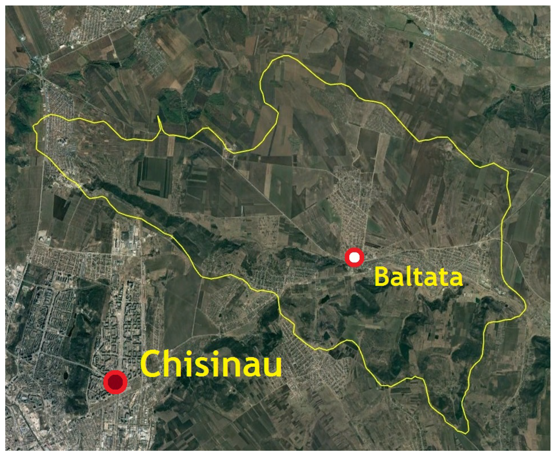
Land 11 00167 g001
Figure 2. The upper part of the Bălțata river, from its source to the hydrological post where flow observations were used for SWAT testing. Note: the watershed line is shown in yellow.
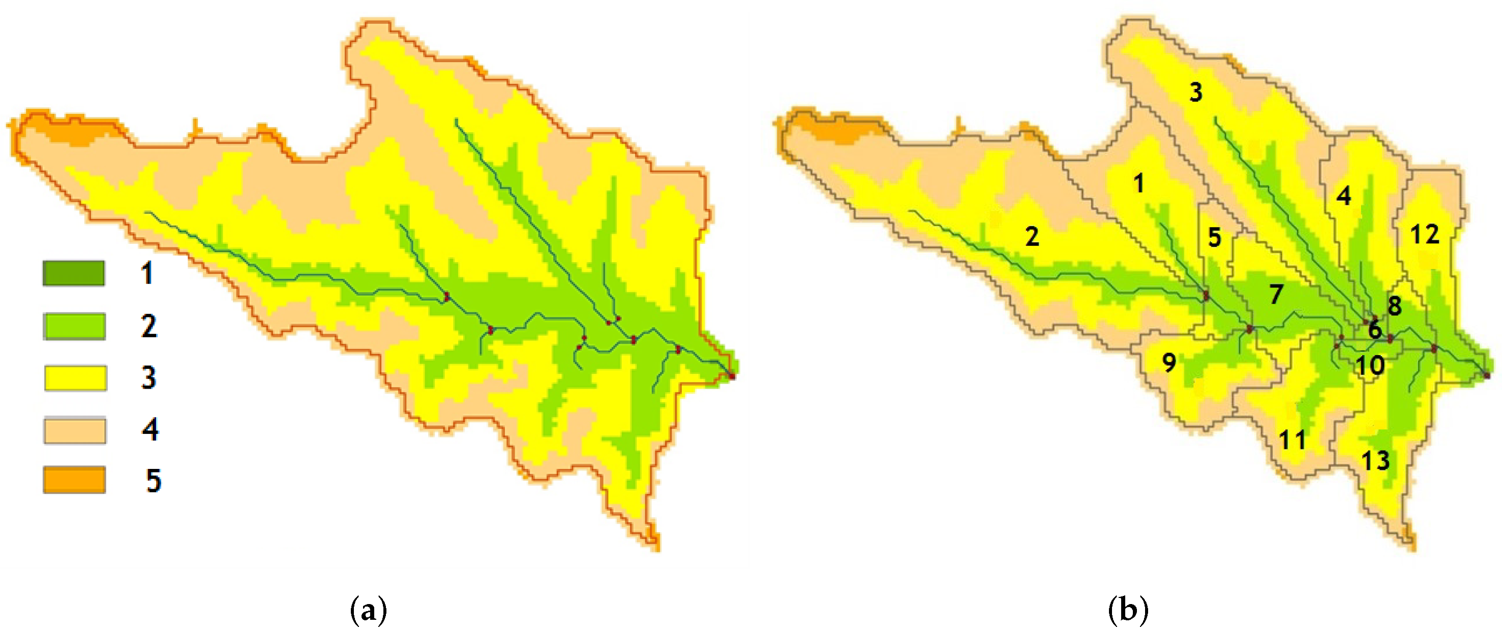
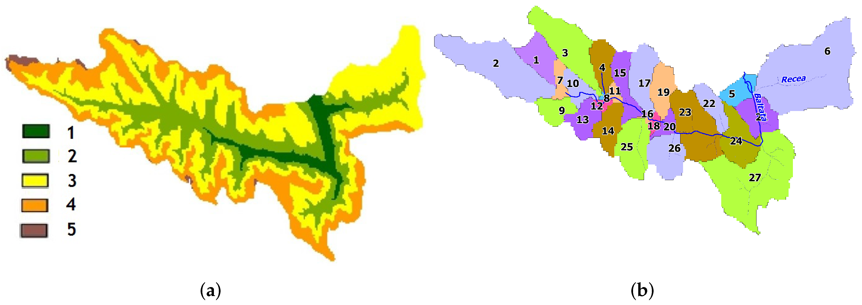
Land 11 00167 g002
Figure 3. The catchment area of the Upper Bălțata, its reaches, and outlet, defined as connection points of streams, overlaid on the digital elevation model (in m) (a) and highlighted sub-basins (b), numbered. Legend—altitude is shown in colour: 1—below 50 m; 2—50–100 m; 3—100–150 m; 4—150–200 m; 5—higher than 200 m.
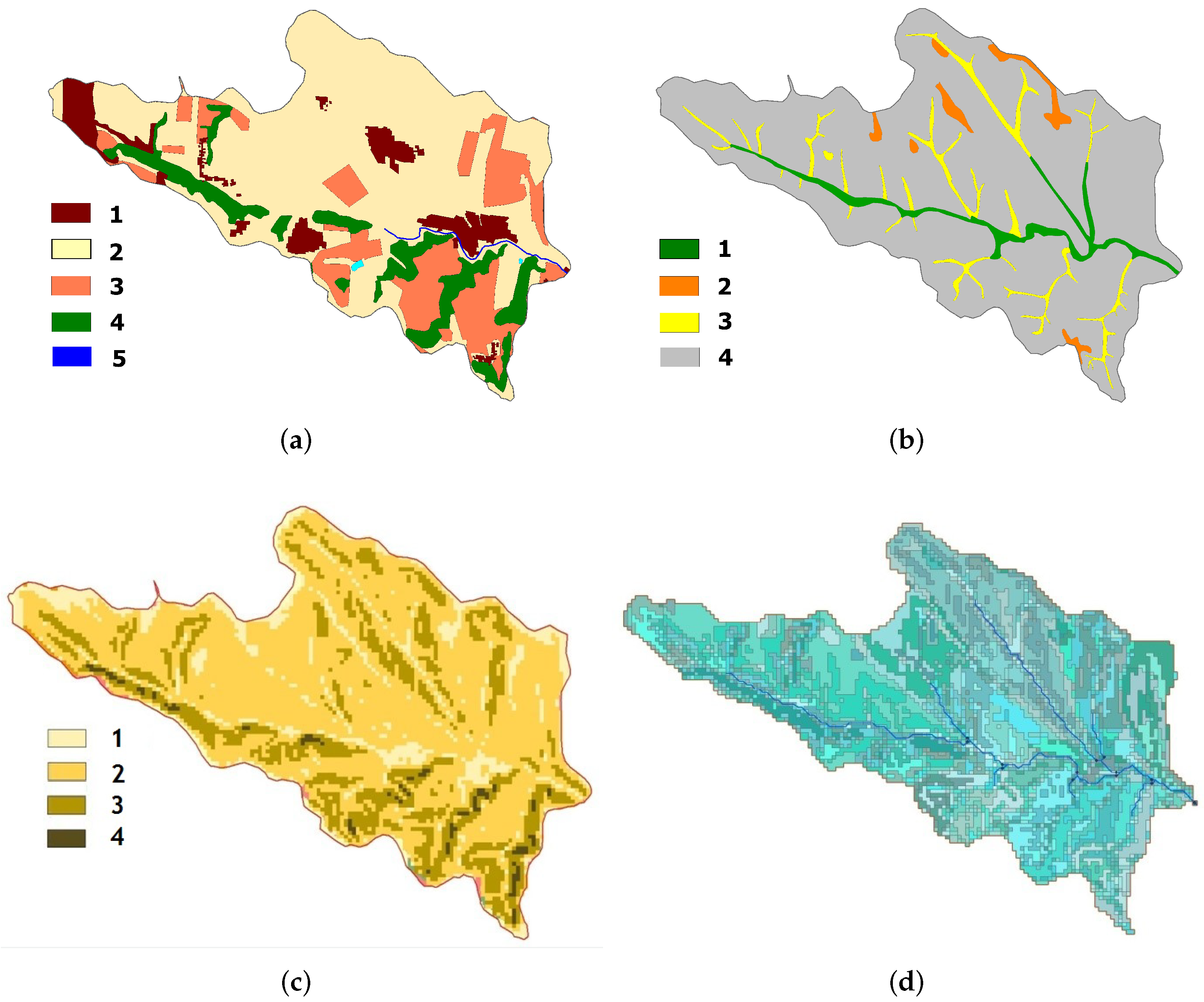
Land 11 00167 g003
Figure 4. Thematic layers for the hydrologic response units’ identification in the Upper Bălțata: (a) land use types; 1—urban fabric, 2—cropland, 3—orchards, 4—forests, 5—water; (b) soil types: 1—fluvisols, 2—vertisols, 3—gleysols, 4—chernozems; (c) slope angles: 1—less than 2°, 2—2–7°, 3—7–12°, 4—more than 12°; (d) overlapping layer (Full HRU).
Land 11 00167 g004
Figure 5. The main channel of the Bălțata River in its particular parts: a pond 2 km southeast of Bălțata village (a), a pond 1.3 km northwest of Cimișeni village (b), a pond 2 km south-ward Bălăbănești village (c), the river mouth (d).
Land 11 00167 g005
Figure 6. The Bălțata River Basin: (a) on a digital elevation model (Legend—altitude is given in colour: 1—below 50 m, 2—50–100 m, 3—100–150 m, 4—150–200 m, 5—higher than 200 m) and (b) split into sub-basins (numbered).
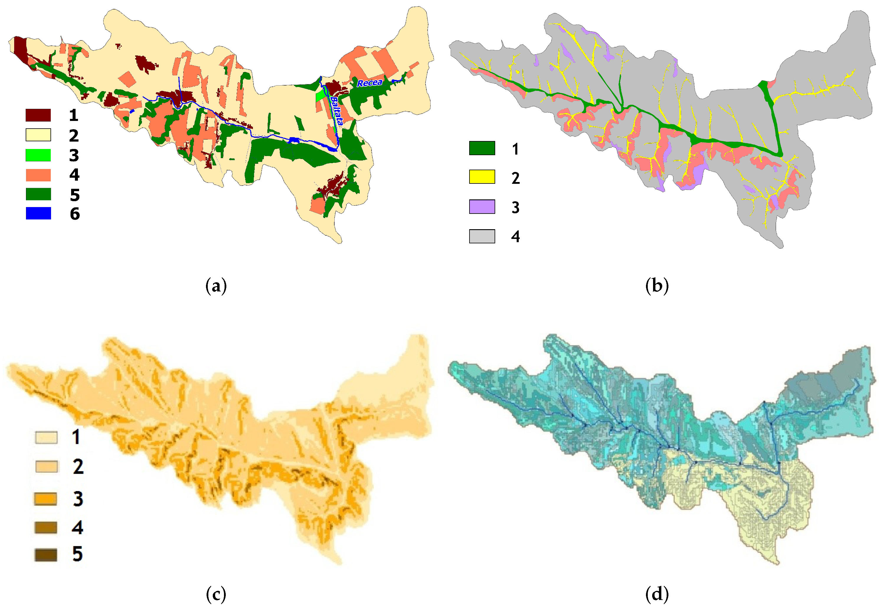
Land 11 00167 g006
Figure 7. Thematic layers for the hydrologic response units’ identification in the Bălțata River Basin: (a) land use types: 1—urban fabric, 2—cropland, 3—pastures, 4—orchards, 5—forests, 6—water; (b) Soil types: 1—fluvisols, 2—vertisols, 3—gleysols, 4—chernozems; (c) Slope angles: 1—less than 2°, 2—2°–7°, 3—7°–12°, 4—more than 12°; (d) overlapping layer (Full HRU).
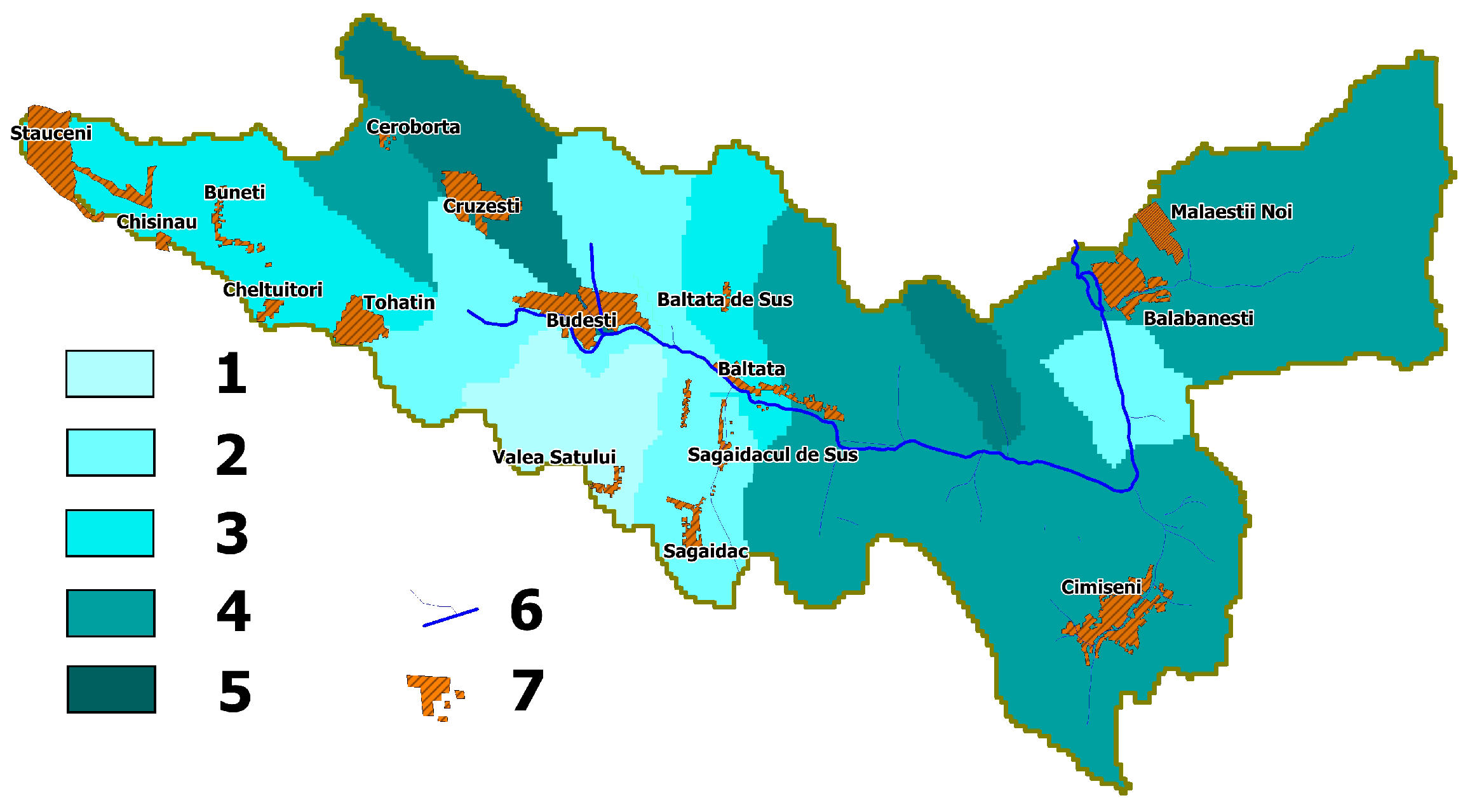
Land 11 00167 g007
Figure 8. Spatial distribution of annual surface runoff in the Bălțata River Basin under a baseline climate. Legend: 1—less than 315 mm, 2—315–318 mm, 3—318–321 mm, 4—321–324 mm, 5—more than 324 mm, 6—main river and its tributaries, 7—settlements.
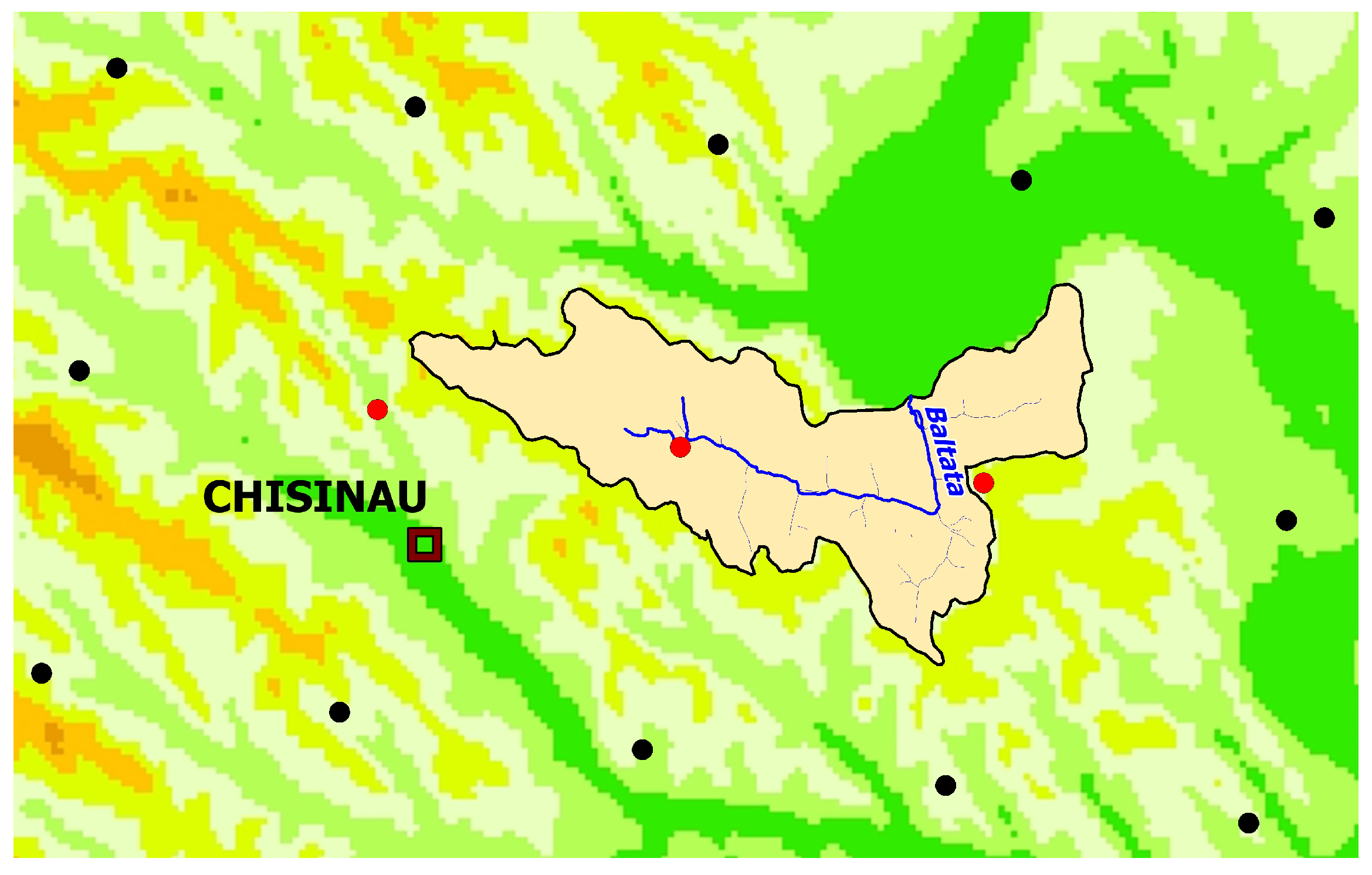
Land 11 00167 g008
Figure 9. Position of the CORDEX nodes (red and black dots) relative to the Bălțata River Basin overlaid on the digital elevation model; red dots represent the nodes, used for this study.
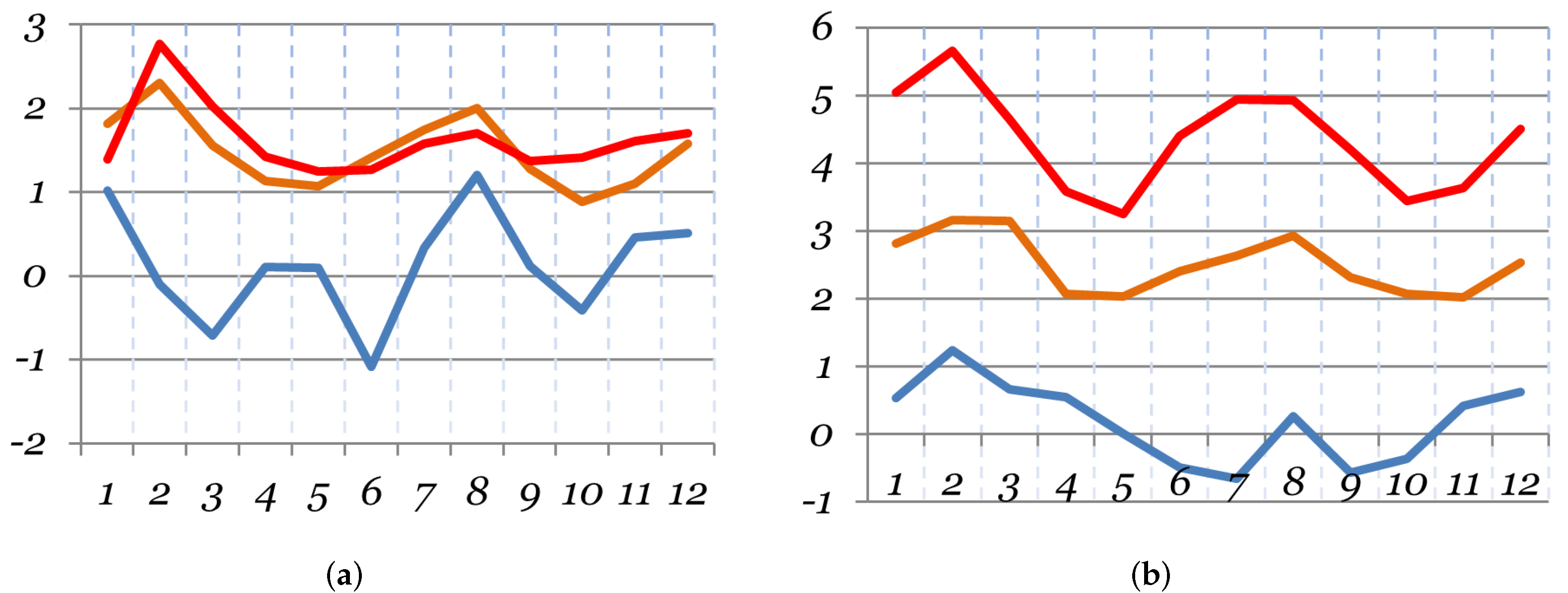
Land 11 00167 g009
Figure 10. The annual trajectory of the projections of average monthly air temperature changes (in °C) in 2021–2050 (a) and 2071–2100 (b) from their base values in 1971–2000 by Representative Concentration Pathways: RCP 2.6 (blue), RCP 4.5 (orange), and RCP 8.5 (red).
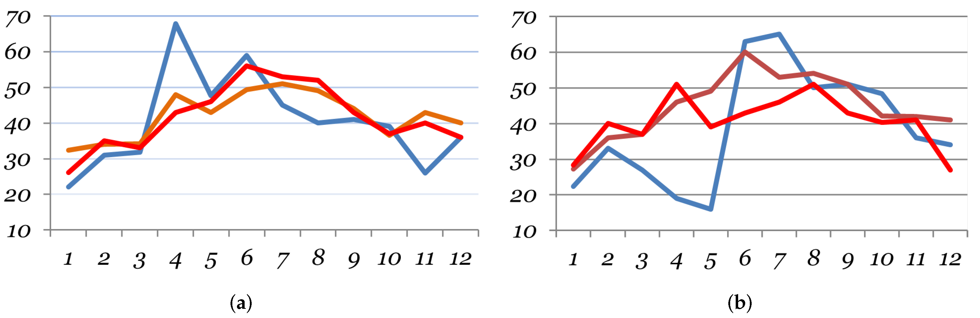
Land 11 00167 g010
Figure 11. The annual trajectory of the projections of monthly precipitation changes (in mm) in 2021–2050 (a) and 2071–2100 (b) compared to their base values in 1971–2000 by the Representative Concentration Pathways: RCP 2.6 (blue), RCP 4.5 (orange), and RCP 8.5 (red).
Land 11 00167 g011
Table 1. Seasonal and yearly mean air temperature (°C) and precipitation (mm) at Bălțata weather station in 1991–2020.
YearAir TemperaturePrecipitation
T m e a n T m a x T m i n
Winter−1.22.3−4.586
Spring10.015.94.4109
Summer20.727.214.3191
Autumn9.915.35.1115
Year10.215.24.8501
Tmean—mean temperature; Tmax—maximum temperature; Tmin—minimum temperature.
Table 2. Monthly water discharge (m 3 /s) at the Bălțata hydrological post in 2006–2010.
YearMonths
123456789101112
20060.0320.0460.0930.0490.0520.0560.0660.0510.0480.0460.0450.005
20070.0530.0540.0660.0490.0450.0370.0290.0220.0370.0470.0480.053
20080.0540.0560.0530.0550.0110.0450.0360.0250.0340.0330.0550.049
20090.0360.0340.0360.0330.0390.0280.0410.0270.0360.0370.0410.043
20100.0470.0720.0360.0400.0370.0370.0360.0330.0360.0390.0370.041
Table 3. Monthly weather observation at Bălțata weather station in 2006–2010.
YearMonthsAnnual
123456789101112
Average monthly maximum temperature, °C
2006−3.70.17.416.622.025.427.928.022.717.610.66.915.1
20078.34.512.916.426.229.432.429.822.215.56.71.917.2
20081.56.813.215.821.126.328.130.120.017.79.54.116.2
20092.35.49.018.522.729.330.328.825.216.610.42.216.7
2010−2.02.69.716.923.227.129.632.022.212.415.31.715.9
Sd3.14.03.62.22.01.71.91.92.11.42.92.61.2
Average monthly minimum temperature, °C
2006−10.6−7.7−1.54.68.913.114.415.310.15.41.7−0.74.4
2007−1.0−3.80.82.911.515.016.716.49.75.5−0.6−1.85.9
2008−4.0−1.81.36.69.513.414.714.89.25.71.3−0.95.8
2009−4.7−1.1−0.22.59.013.416.313.79.66.92.6−4.15.3
2010−7.7−2.8−1.93.910.514.817.016.99.92.85.4−5.85.3
Sd3.23.22.01.41.20.91.31.11.11.43.02.70.7
Average precipitation, mm
2006252262398074918056841542
200738453640115973226735148466
200818344437735523870261644466
200915185534729111122731672426
20106944194763100563946553775650
Sd18.817.219.621.226.945.737.242.538.225.922.518.099.1
Table 4. Results of the SWAT simulation in the Upper Bălțata watershed.
YearSWAT Output Data, mm
PRECRunoff in the Main ChannelInfiltration in SoilEvapotranspirationWATER YIELD
SURQLATQGWQLATESWETPET
2006542109.7177.540.059.03.8118.3738.8329.0
200746694.5148.630.348.53.8110.0741.5274.9
200846693.2151.130.649.03.7109.7741.1276.4
200942685.5134.425.943.83.8104.3742.7247.1
2010501101.3161.534.453.03.8114.6740.9298.9
Average48096.8154.632.250.63.8111.4741.0285.2
Abbreviations: RREC—The average amount of simulated precipitation; SURQ—Surface runoff contribution to streamflow; LATQ—Lateral flow contribution to streamflow; GWQ—Groundwater contribution to streamflow; LATE—Water percolation past the bottom of the soil profile; SW—Water amount stored in the soil profile; ET—Actual evapotranspiration; PET—Potential evapotranspiration; WATER YIELD—Water yield to streamflow.
Table 5. Comparison of the observed and simulated Upper Bălțata River runoff into its main channel.
YearMonthsYear
123456789101112
Observed runoff, t h o u . m 3
200682.9111.3249.1127.0139.3145.2176.8136.6124.4123.2116.613.41545.8
2007137.4130.6176.8127.0120.595.977.758.995.9125.9124.4142.01413.0
2008140.0135.5142.0142.629.5116.696.467.088.188.4142.6131.21319.9
200993.382.396.485.5104.572.6109.872.393.399.1106.3115.21130.5
2010121.8174.296.4103.799.196.096.488.393.3104.595.9109.81279.4
Modelling runoff, t h o u . m 3
20060.0862.2108.4822.91000.5522.9855.17025.94564.61100.2672.1384.517,919.2
20070.0644.364.8541.4796.8307.2547.46094.04256.4917.2501.1302.314,972.7
20080.0644.965.4559.9808.3293.6546.36115.84264.5913.9487.4354.115,053.8
20090.0574.634.9372.0693.9215.1413.95583.64048.3822.9428.1268.513,455.9
20100.0726.681.7660.6891.0397.0671.56527.04405.6999.4580.0336.016,276.6
The ratio of the observed to simulated flows
20060.1292.2980.1540.1390.2780.2070.0190.0270.1120.1740.0350.086
20070.2032.7270.2350.1510.3120.1420.0100.0230.1370.2480.4700.094
20080.1281.4750.1530.1290.2470.2010.0120.0220.1080.2180.3250.075
20090.1432.7660.2300.1510.3370.2650.0130.0230.1200.2480.4290.084
20100.2401.1800.1570.1110.2420.1440.0140.0210.1050.1650.3270.079
Table 6. Change in runoff from the Cogilnic River catchment with a consecutive 10% reduction in the CN2 [25].
CN2201020112012
SURQLATQGWQYieldSURQLATQGWQYieldSURQLATQGWQYield
78.8131.970.9100.9307.741.562.185.4193.143.561.984.4193.4
71.091.577.6128.8303.016.366.6101.0188.8190.066.890.1191.2
63.169.881.1144.2300.86.468.5107.2187.26.568.3106.5186.4
56.255.483.3154.7299.64.269.0108.7187.04.068.8108.2186.2
Table 7. Area of the Bălțata River sub-basins.
No.S, haNo.S, haNo.S, ha
1465.7510286.7419419.58
21577.071182.6220153.09
31009.261262.3721474.66
4382.3213366.9322341.01
5289.1714411.4823997.92
62597.6715452.7924631.80
7168.481623.4925656.10
823.4917575.9126566.19
9324.001877.76271969.92
Table 8. Average monthly air temperature and precipitation at Bălțata weather station in 1981–2010.
Climatic VariableMonths
123456789101112
Tmax, °C1.33.08.716.322.725.828.027.822.215.77.92.6
Sd3.14.03.62.22.01.71.91.92.11.42.92.6
Tmin, °C−5.2−4.6−0.94.59.513.415.214.49.84.90.5−3.7
Sd3.23.22.01.41.20.91.31.11.11.43.02.7
Precipitation, mm282530374371635645383232
Table 9. SWAT modelling of monthly runoff in the Bălțata River Basin and its accumulation in the artificial ponds in 1981–2010.
PondsMonthsRunoff
123456789101112mmkm 3
Bălțata Pond I0.052.13.71.50.093.69.19.65.83.26.20.044.940.004349
Bălțata Pond II0.094.47.52.11.66.517.817.711.75.712.60.287.890.009341
Cimișeni Pond0.146.511.23.62.610.126.727.317.58.918.80.2133.540.017197
Bălăbănești Pond0.021.42.10.70.061.65.65.13.92.64.10.027.180.000393
Runoff into ponds0.314.424.57.94.3521.859.259.738.920.441.70.4293.550.031280
Watershed0.415.127.48.94.623.162.263.040.421.644.50.5311.80.047990
Table 10. Projections of mean air temperatures’ change in the Bălțata River Basin for different Representative Concentration Pathways (RCPs) and time horizons, in °C.
SeasonBaselineProjections for RCPs and Time Horizons
RCP 2.6RCP 4.5RC P8.5
1971–20002021–20502071–21002021–20502071–21002021–20502071–2100
Winter−2.00.50.81.92.82.05.1
Spring9.4−0.20.41.22.41.63.8
Summer19.70.2−0.31.72.71.54.8
Autumn9.10.1−0.21.12.11.53.8
Year9.10.10.21.52.51.64.4
Table 11. Simple linear regression analysis of the relationships between monthly maximum and minimum air temperatures vs. mean air temperature at Bălțata weather station in 1961–2010.
SeasonMean Maximum TemperatureMean Minimum Temperature
R 2 r r 0 r 1 sd R 2 r r 0 r 1 sd
Winter95.20.9763.421.0110.4492.90.964−3.280.9250.49
Spring96.20.9812.251.3600.3571.50.845−1.460.6030.49
Summer94.80.9741.131.2570.3170.00.8411.460.6250.43
Autumn78.90.8884.151.1260.6163.80.799−3.140.8320.65
Year89.90.9475.830.9220.3573.00.854−0.500.5370.37
R2—coefficient of determination; r—correlation coefficient; r0—intersection; r1—regression coefficient; sd—standard error. Statistical significance of all models, expressed as a p-value, is less than 0.001.
Table 12. Projections of changes of maximum and minimum air temperatures (°C) relative to 1971–2000 by season.
SeasonBaselineRCP 2.6RCP 4.5RCP 8.5
2021–20502071–21002021–20502071–21002021–20502071–2100
Maximum temperature, °C
Winter2.10.50.92.13.12.25.5
Spring15.3−0.20.41.83.42.25.2
Summer26.40.2−0.22.03.31.75.5
Autumn14.90.20.01.22.31.64.1
Year14.70.20.31.83.11.95.2
Minimum temperature, °C
Winter−4.60.50.92.13.12.15.2
Spring4.4−0.10.20.91.61.12.5
Summer14.00.1−0.11.42.31.23.9
Autumn4.80.10.01.02.01.43.4
Year4.60.10.21.32.11.43.5
Table 13. Projections of precipitation change in absolute (mm) and relative (%) figures in the Bălțata River Basin compared to 1971–2000 by season.
SeasonBaselineRCP 2.6RCP 4.5RCP 8.5
1971–20002021–20502071–21002021–20502071–21002021–20502071–2100
mmmm%mm%mm%mm%mm%mm%
Winter8544.744.72124.71922.41216.61011.8
Spring1173021.93025.585.81512.854.38.514.6
Summer193−49−25.4−15−7.8−44−22.8−26−13.5−32−16.6−53−27.5
August118−12−10.2175.765.11714.421.765.1
Year512−26−5.1367.0−7−1.4265.1−12−2.3254.9
Table 14. Projection of monthly air temperature and precipitation in the Bălțata River Basin.
Time HorizonRCPMonthsYear
123456789101112
Maximum temperature, °C
2021–2050RCP 2.61.72.36.916.322.324.127.428.322.115.010.13.215.0
RCP 4.52.55.09.917.723.527.229.229.323.716.311.14.216.6
RCP 8.52.15.510.518.023.727.029.028.923.916.911.94.316.8
2071–2100RCP 2.61.33.88.716.922.124.826.227.121.215.010.03.315.0
RCP 4.53.55.912.118.924.728.530.330.525.217.612.65.117.9
RCP 8.55.68.714.020.826.331.033.133.027.819.015.27.020.1
Minimum temperature, °C
2021–2050RCP 2.6−4.8−4.8−1.64.79.612.715.014.89.64.20.6−2.84.8
RCP 4.5−4.0−2.40.05.410.214.116.015.310.35.51.2−1.85.8
RCP 8.5−4.4−2.00.45.610.314.015.915.110.36.01.7−1.65.9
2071–2100RCP 2.6−5.3−3.5−0.65.09.613.014.414.19.34.30.5−2.74.8
RCP 4.5−2.9−1.61.26.010.814.616.615.910.86.62.1−0.86.6
RCP 8.5−0.60.92.37.011.515.818.217.211.97.93.71.18.1
Precipitation, mm
2021–2050RCP 2.6223132684859454041392636487
RCP 4.5323434484349514944374340505
RCP 8.5263533434656535243374036500
2071–2100RCP 2.6223327191663655051483634465
RCP 4.5273637464960535451424241538
RCP 8.5284037513943465143404127487
Table 15. Modelling projections of changes in the Bălțata watershed in absolute (mm) and relative values (%) compared to 1981–2010.
MonthBaselineRCP2.6RCP4.5RCP8.5
1981–20102021–20502071–21002021–20502071–21002021–20502071–2100
mmmm%mm%mm%mm%mm%mm%
January0.40.246.3−0.4−1000.7158.5−0.4−1000.6136.6−0.4−100
February15.12.617.0−10.2−67.57.650.1−8.8−58.17.348.1−9.5−62.9
March27.41.24.2−9.4−34.46.021.8−4.4−15.95.821.2−8.0−29.2
April8.913.5152.1−8.9−99.95.663.4−8.8−98.65.258.9−8.9−99.8
May4.66.8148.5−4.6−99.81.736.5−4.6−99.61.532.2−4.6−99.8
June23.14.620.0−22.1−95.8−2.1−9.0−21.4−92.5−2.8−11.9−22.0−95.3
July62.2−17.0−27.4−53.6−86.2−6.3−10.1−47.4−76.2−6.8−10.9−51.7−83.1
August63.0−20.2−32.0−43.1−68.4−4.8−7.7−36.4−57.7−5.2−8.2−41.1−65.2
September40.4−8.6−21.2−21.8−53.9−1.7−4.2−14.8−36.6−1.8−4.5−19.7−48.8
October21.6−6.1−28.3−7.2−33.1−3.2−14.9−1.2−5.3−3.3−15.4−5.4−25.0
November44.5−9.0−20.297.8219.923.152.0115.7260.122.550.6104.1234.1
December0.5−0.1−12.54.49170.0−2.15.711960.0−2.14.8991.7
Year311.8−32.0−10.3−79.2−25.426.58.5−26.6−8.523.07.4−62.4−20.0
Table 16. Modelling projections of changes in the Bălțata watershed runoff into artificial ponds in absolute (mm) and relative expression (%) compared to 1981–2010.
PondBaselineRCP2.6RCP4.5RCP8.5
1981–20102021–20502071–21002021–20502071–21002021–20502071–2100
mmmm%mm%mm%mm%mm%mm%
Bălțata Pond I44.94−4.6−10.3−11.4−25.43.88.5−3.8−8.53.37.4−9.0−20.0
Bălțata Pond II87.89−9.1−10.3−22.3−25.47.58.5−7.5−8.56.57.4−17.6−20.0
Cimișeni Pond133.54−13.8−10.3−33.9−25.411.48.5−11.5−8.59.97.4−26.7−20.0
Bălăbănești Pond27.18−2.8−10.3−6.9−25.42.38.5−2.3−8.52.07.4−5.4−20.0
Runoff into ponds293.55−30.2−10.3−74.6−25.424.98.5−24.9−8.521.77.4−58.7−20.0
Publisher’s Note: MDPI stays neutral with regard to jurisdictional claims in published maps and institutional affiliations.

