

Spatial-Temporal Characteristics and Influencing Factors of Particulate Matter: Geodetector Approach

Abstract
:1. Introduction
2. Literature Review
2.1. Main Causes of Respirable Particulate Matter
2.2. Influencing Factors of Particulate Matter Distribution
2.3. Summary
3. Materials and Methods
3.1. Research Implementation Process
3.2. Study Area and Materials
3.3. Methods
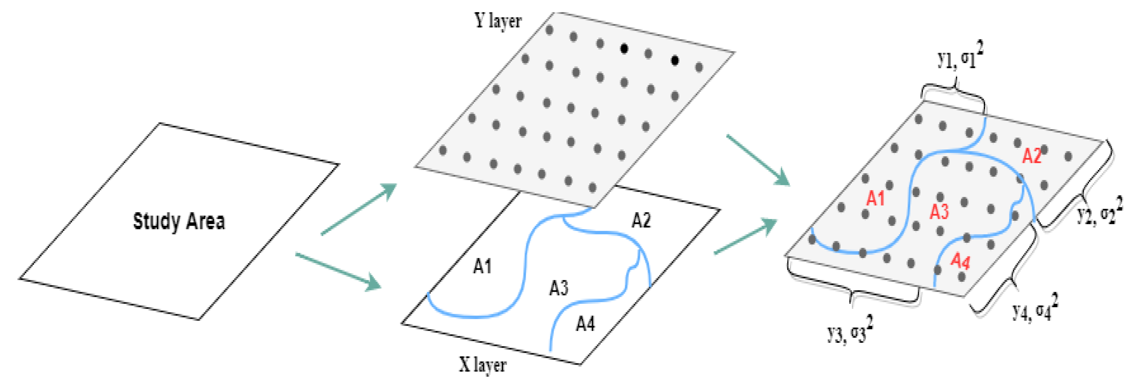
3.3.1. LISA Analysis
3.3.2. Geodetector
4. Results
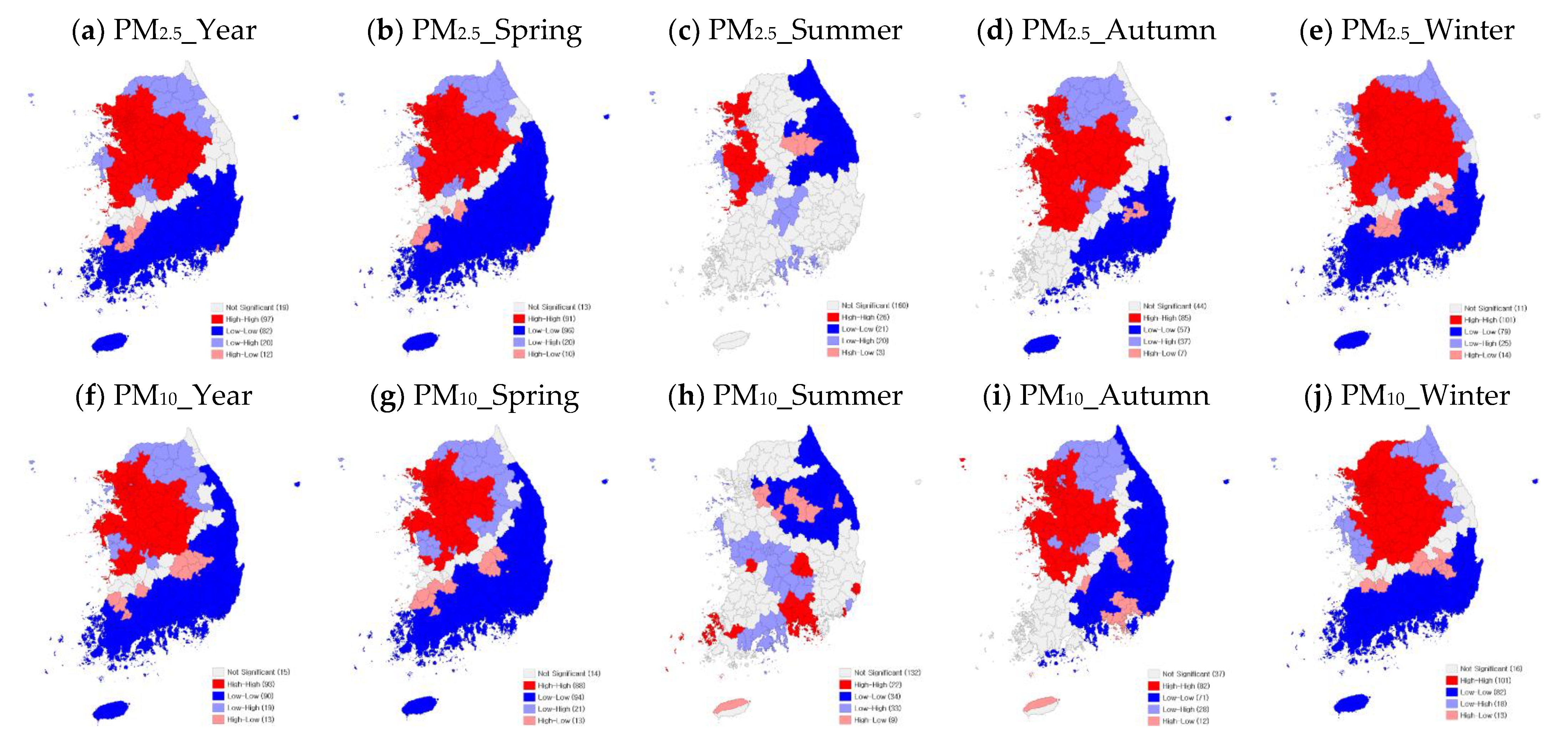
4.1. LISA Results
4.2. Geodetector Results
4.2.1. Factor Detector
4.2.2. Risk Detector
4.2.3. Interaction Detector
5. Conclusions
Author Contributions
Funding
Data Availability Statement
Conflicts of Interest
Appendix A. Natural Break Classify
 |
 |
 |
Appendix B. The Risk Detection of the Influencing Factors to PM10 & PM2.5
 |
 |
Appendix C. The Results of the Interaction Detection for the Influencing Factors of Urban PM10 in 2019
| XP1 | XP2 | XP3 | XP4 | XP5 | XP6 | XS1 | XS2 | XS3 | XS4 | XL1 | XL2 | XL3 | XL4 | XL5 | XL6 | XL7 | XL8 | ||||
| XP1 | 0.2183 | ||||||||||||||||||||
| XP2 | 0.2553 | 0.1695 | |||||||||||||||||||
| XP3 | 0.2917 | 0.2611 | 0.1031 | ||||||||||||||||||
| XP4 | 0.3540 | 0.3552 | 0.2169 | 0.0835 | |||||||||||||||||
| XP5 | 0.4059 | 0.3794 | 0.2162 | 0.1115 | 0.0772 | ||||||||||||||||
| XP6 | 0.3069 | 0.3393 | 0.2441 | 0.3214 | 0.3556 | 0.1728 | |||||||||||||||
| XS1 | 0.3643 | 0.3083 | 0.3264 | 0.2964 | 0.2648 | 0.3330 | 0.1100 | ||||||||||||||
| XS2 | 0.3424 | 0.3117 | 0.2527 | 0.2972 | 0.2502 | 0.3175 | 0.2868 | 0.1094 | |||||||||||||
| XS3 | 0.2789 | 0.3070 | 0.1310 | 0.1836 | 0.1619 | 0.2258 | 0.1791 | 0.1499 | 0.0119 | ||||||||||||
| XS4 | 0.2586 | 0.2139 | 0.1959 | 0.2648 | 0.2608 | 0.2039 | 0.2783 | 0.2759 | 0.1668 | 0.1265 | |||||||||||
| XL1 | 0.2867 | 0.2468 | 0.1630 | 0.2878 | 0.2540 | 0.1944 | 0.2480 | 0.2760 | 0.1884 | 0.2172 | 0.1416 | ||||||||||
| XL2 | 0.3025 | 0.3059 | 0.2453 | 0.3069 | 0.3144 | 0.2701 | 0.3385 | 0.3134 | 0.2899 | 0.2418 | 0.2293 | 0.2242 | |||||||||
| XL3 | 0.3011 | 0.2526 | 0.1907 | 0.1347 | 0.1239 | 0.2650 | 0.1747 | 0.1777 | 0.0788 | 0.2162 | 0.2219 | 0.2845 | 0.0680 | ||||||||
| XL4 | 0.4696 | 0.3903 | 0.4395 | 0.4055 | 0.3732 | 0.4571 | 0.3675 | 0.4025 | 0.3561 | 0.4754 | 0.3961 | 0.3975 | 0.3375 | 0.2905 | |||||||
| XL5 | 0.2962 | 0.2384 | 0.1431 | 0.1964 | 0.1713 | 0.2191 | 0.1695 | 0.2113 | 0.0681 | 0.2201 | 0.1908 | 0.2866 | 0.1146 | 0.3646 | 0.0383 | ||||||
| XL6 | 0.3326 | 0.2793 | 0.1788 | 0.2401 | 0.1512 | 0.2749 | 0.1886 | 0.1637 | 0.0686 | 0.2865 | 0.2667 | 0.3219 | 0.1267 | 0.3967 | 0.1276 | 0.0253 | |||||
| XL7 | 0.3785 | 0.3692 | 0.2860 | 0.2217 | 0.1993 | 0.3930 | 0.2966 | 0.2603 | 0.1730 | 0.3087 | 0.2956 | 0.4012 | 0.2001 | 0.4148 | 0.2081 | 0.3331 | 0.1150 | ||||
| XL8 | 0.3885 | 0.3409 | 0.3009 | 0.2919 | 0.2577 | 0.3055 | 0.2485 | 0.2581 | 0.1555 | 0.3160 | 0.3064 | 0.3243 | 0.1704 | 0.4272 | 0.1792 | 0.1516 | 0.3200 | 0.0682 | |||
| XE1 | 0.4809 | 0.5172 | 0.3713 | 0.4106 | 0.3999 | 0.4555 | 0.3699 | 0.3952 | 0.2947 | 0.4822 | 0.3847 | 0.4559 | 0.2173 | 0.5075 | 0.2831 | 0.2850 | 0.4063 | 0.3567 | |||
| XE2 | 0.5419 | 0.5011 | 0.4649 | 0.4905 | 0.5022 | 0.4949 | 0.5968 | 0.5566 | 0.5576 | 0.5070 | 0.5173 | 0.5309 | 0.4215 | 0.5870 | 0.5106 | 0.4862 | 0.5292 | 0.5421 | |||
| XE3 | 0.4896 | 0.4654 | 0.3629 | 0.4806 | 0.4950 | 0.4540 | 0.3487 | 0.3908 | 0.2184 | 0.4292 | 0.3758 | 0.5031 | 0.2031 | 0.4577 | 0.2497 | 0.2743 | 0.4162 | 0.3290 | |||
| XE4 | 0.5225 | 0.5183 | 0.4100 | 0.4419 | 0.3532 | 0.4935 | 0.4296 | 0.4469 | 0.3486 | 0.4968 | 0.4791 | 0.4987 | 0.3037 | 0.5668 | 0.4181 | 0.4387 | 0.4246 | 0.4192 | |||
| XE5 | 0.3997 | 0.4545 | 0.4797 | 0.5421 | 0.5128 | 0.4602 | 0.5775 | 0.5226 | 0.4721 | 0.4883 | 0.4600 | 0.4481 | 0.3849 | 0.5436 | 0.4334 | 0.4688 | 0.5180 | 0.5625 | |||
| XE6 | 0.4280 | 0.3897 | 0.2633 | 0.4143 | 0.3768 | 0.3346 | 0.4189 | 0.3818 | 0.3369 | 0.3526 | 0.3000 | 0.4313 | 0.2848 | 0.4910 | 0.2780 | 0.4120 | 0.4319 | 0.4565 | |||
| XE7 | 0.2702 | 0.2315 | 0.1742 | 0.1748 | 0.1635 | 0.2482 | 0.2008 | 0.2019 | 0.1022 | 0.1988 | 0.2110 | 0.2725 | 0.1539 | 0.3426 | 0.1245 | 0.1184 | 0.2214 | 0.1514 | |||
| XT1 | 0.2556 | 0.2486 | 0.3114 | 0.3401 | 0.3662 | 0.3386 | 0.3593 | 0.3319 | 0.2793 | 0.2880 | 0.2769 | 0.3198 | 0.3203 | 0.4009 | 0.2788 | 0.3327 | 0.3508 | 0.3722 | |||
| XT2 | 0.2900 | 0.3018 | 0.2421 | 0.2985 | 0.2966 | 0.2554 | 0.3212 | 0.3140 | 0.2266 | 0.2333 | 0.2114 | 0.2757 | 0.2552 | 0.3750 | 0.2396 | 0.3169 | 0.3338 | 0.3087 | |||
| XT3 | 0.3306 | 0.2889 | 0.1789 | 0.2673 | 0.2606 | 0.2211 | 0.2161 | 0.3330 | 0.1861 | 0.1851 | 0.1806 | 0.2744 | 0.1896 | 0.3491 | 0.1489 | 0.2059 | 0.3017 | 0.2618 | |||
| XT4 | 0.2776 | 0.2539 | 0.2012 | 0.3318 | 0.3373 | 0.2836 | 0.3407 | 0.3342 | 0.2118 | 0.2160 | 0.1989 | 0.2521 | 0.2479 | 0.3983 | 0.2106 | 0.2178 | 0.3727 | 0.2443 | |||
| XT5 | 0.3064 | 0.2974 | 0.3243 | 0.3366 | 0.3610 | 0.3456 | 0.3615 | 0.3743 | 0.3214 | 0.3048 | 0.2735 | 0.3330 | 0.3311 | 0.4525 | 0.2947 | 0.3134 | 0.3730 | 0.3816 | |||
| XG1 | 0.3470 | 0.3312 | 0.3113 | 0.2697 | 0.2351 | 0.3825 | 0.2420 | 0.2731 | 0.1256 | 0.2444 | 0.2161 | 0.2868 | 0.1695 | 0.3760 | 0.1489 | 0.2235 | 0.2894 | 0.2764 | |||
| XG2 | 0.2897 | 0.2709 | 0.2479 | 0.3842 | 0.3802 | 0.2393 | 0.2845 | 0.3434 | 0.2989 | 0.2306 | 0.2165 | 0.2600 | 0.2651 | 0.4586 | 0.2816 | 0.2828 | 0.3799 | 0.3277 | |||
| XG3 | 0.3195 | 0.3519 | 0.2737 | 0.3821 | 0.3821 | 0.3062 | 0.3691 | 0.3574 | 0.3522 | 0.2558 | 0.2584 | 0.3574 | 0.2693 | 0.4828 | 0.2492 | 0.3470 | 0.4155 | 0.4043 | |||
| XG4 | 0.3146 | 0.2782 | 0.2707 | 0.3129 | 0.2989 | 0.2949 | 0.3149 | 0.2921 | 0.1880 | 0.2873 | 0.2290 | 0.2823 | 0.2467 | 0.4572 | 0.1977 | 0.3276 | 0.3243 | 0.4047 | |||
| XG5 | 0.2610 | 0.2568 | 0.3033 | 0.3490 | 0.3931 | 0.3246 | 0.3749 | 0.3419 | 0.3185 | 0.2655 | 0.3047 | 0.3055 | 0.3061 | 0.4736 | 0.2792 | 0.3321 | 0.3693 | 0.3918 | |||
| XE1 | XE2 | XE3 | XE4 | XE5 | XE6 | XE7 | XT1 | XT2 | XT3 | XT4 | XT5 | XG1 | XG2 | XG3 | XG4 | XG5 | |||||
| XE1 | 0.1436 | ||||||||||||||||||||
| XE2 | 0.6857 | 0.3759 | |||||||||||||||||||
| XE3 | 0.5667 | 0.7550 | 0.1317 | ||||||||||||||||||
| XE4 | 0.5821 | 0.5618 | 0.6428 | 0.2355 | |||||||||||||||||
| XE5 | 0.7535 | 0.5499 | 0.6714 | 0.5527 | 0.3428 | ||||||||||||||||
| XE6 | 0.5239 | 0.5567 | 0.5451 | 0.5200 | 0.5934 | 0.1993 | |||||||||||||||
| XE7 | 0.2266 | 0.4238 | 0.2203 | 0.3288 | 0.3962 | 0.2566 | 0.0856 | ||||||||||||||
| XT1 | 0.5078 | 0.5188 | 0.5280 | 0.5004 | 0.4287 | 0.3804 | 0.2675 | 0.2199 | |||||||||||||
| XT2 | 0.3849 | 0.5239 | 0.3924 | 0.4593 | 0.4471 | 0.3209 | 0.2503 | 0.2909 | 0.1920 | ||||||||||||
| XT3 | 0.3517 | 0.4961 | 0.3551 | 0.4597 | 0.4704 | 0.3141 | 0.1928 | 0.3299 | 0.2724 | 0.1269 | |||||||||||
| XT4 | 0.4524 | 0.5336 | 0.4109 | 0.4013 | 0.4499 | 0.3242 | 0.2144 | 0.2557 | 0.2515 | 0.2627 | 0.1517 | ||||||||||
| XT5 | 0.5164 | 0.5243 | 0.5242 | 0.5180 | 0.4103 | 0.4170 | 0.2802 | 0.2602 | 0.3216 | 0.3422 | 0.2802 | 0.2314 | |||||||||
| XG1 | 0.3813 | 0.4967 | 0.4637 | 0.3708 | 0.5254 | 0.3717 | 0.1718 | 0.3733 | 0.2702 | 0.2149 | 0.2496 | 0.3463 | 0.0917 | ||||||||
| XG2 | 0.4739 | 0.5002 | 0.4499 | 0.5008 | 0.4612 | 0.4016 | 0.2407 | 0.2811 | 0.2934 | 0.2693 | 0.2683 | 0.2971 | 0.2760 | 0.1829 | |||||||
| XG3 | 0.5235 | 0.4759 | 0.5156 | 0.4998 | 0.4870 | 0.3984 | 0.2827 | 0.3184 | 0.2636 | 0.2862 | 0.3269 | 0.3422 | 0.3906 | 0.3372 | 0.2181 | ||||||
| XG4 | 0.4401 | 0.4858 | 0.4677 | 0.4920 | 0.4027 | 0.3389 | 0.2345 | 0.3267 | 0.2439 | 0.2621 | 0.2516 | 0.3458 | 0.2673 | 0.2871 | 0.2662 | 0.1627 | |||||
| XG5 | 0.4883 | 0.5352 | 0.4851 | 0.5317 | 0.3827 | 0.4351 | 0.2779 | 0.2879 | 0.3215 | 0.3248 | 0.2547 | 0.2890 | 0.3889 | 0.2867 | 0.3157 | 0.2840 | 0.2250 | ||||
Appendix D. The Results of the Interaction Detection for the Influencing Factors of Urban PM2.5 in 2019
| XP1 | XP2 | XP3 | XP4 | XP5 | XP6 | XS1 | XS2 | XS3 | XS4 | XL1 | XL2 | XL3 | XL4 | XL5 | XL6 | XL7 | XL8 | |
| XP1 | 0.0950 | |||||||||||||||||
| XP2 | 0.1232 | 0.0724 | ||||||||||||||||
| XP3 | 0.1836 | 0.1825 | 0.0402 | |||||||||||||||
| XP4 | 0.2222 | 0.2396 | 0.1493 | 0.0379 | ||||||||||||||
| XP5 | 0.2910 | 0.2525 | 0.1345 | 0.0450 | 0.0280 | |||||||||||||
| XP6 | 0.1617 | 0.2154 | 0.1590 | 0.2368 | 0.2842 | 0.0917 | ||||||||||||
| XS1 | 0.2171 | 0.1971 | 0.2363 | 0.2307 | 0.1773 | 0.2078 | 0.0569 | |||||||||||
| XS2 | 0.2484 | 0.2047 | 0.1885 | 0.2598 | 0.2358 | 0.2195 | 0.2336 | 0.1026 | ||||||||||
| XS3 | 0.2119 | 0.2222 | 0.0790 | 0.1429 | 0.1247 | 0.1887 | 0.1151 | 0.1546 | 0.0063 | |||||||||
| XS4 | 0.1223 | 0.1060 | 0.1360 | 0.1860 | 0.1921 | 0.1125 | 0.2012 | 0.2208 | 0.0993 | 0.0592 | ||||||||
| XL1 | 0.2122 | 0.1685 | 0.0681 | 0.1419 | 0.1237 | 0.0986 | 0.1532 | 0.1936 | 0.1414 | 0.1584 | 0.0525 | |||||||
| XL2 | 0.1610 | 0.1754 | 0.1342 | 0.1745 | 0.1689 | 0.1737 | 0.2011 | 0.2234 | 0.2029 | 0.1368 | 0.1264 | 0.1082 | ||||||
| XL3 | 0.1997 | 0.1729 | 0.1679 | 0.1317 | 0.1139 | 0.2115 | 0.1570 | 0.2045 | 0.1013 | 0.2062 | 0.1690 | 0.2182 | 0.0832 | |||||
| XL4 | 0.3122 | 0.2667 | 0.2752 | 0.2762 | 0.2464 | 0.3077 | 0.2430 | 0.2957 | 0.2627 | 0.3399 | 0.2336 | 0.2512 | 0.2770 | 0.1710 | ||||
| XL5 | 0.1525 | 0.1449 | 0.0577 | 0.1438 | 0.0964 | 0.1304 | 0.1160 | 0.1862 | 0.0452 | 0.1291 | 0.1029 | 0.1601 | 0.1307 | 0.2534 | 0.0106 | |||
| XL6 | 0.2552 | 0.1953 | 0.1365 | 0.1842 | 0.1197 | 0.2164 | 0.1428 | 0.1927 | 0.0750 | 0.2455 | 0.2017 | 0.2328 | 0.1690 | 0.2990 | 0.1047 | 0.0322 | ||
| XL7 | 0.2607 | 0.2382 | 0.2109 | 0.1803 | 0.1406 | 0.3285 | 0.2102 | 0.2205 | 0.1463 | 0.2874 | 0.2018 | 0.2697 | 0.1976 | 0.2852 | 0.1619 | 0.2954 | 0.0866 | |
| XL8 | 0.2760 | 0.2469 | 0.2137 | 0.2414 | 0.1946 | 0.2679 | 0.1759 | 0.2332 | 0.1612 | 0.2509 | 0.2419 | 0.2183 | 0.1898 | 0.3121 | 0.1320 | 0.1202 | 0.2751 | 0.0603 |
| XE1 | 0.3693 | 0.4244 | 0.2705 | 0.3673 | 0.3680 | 0.3291 | 0.2708 | 0.3895 | 0.2513 | 0.4092 | 0.2861 | 0.3153 | 0.2228 | 0.4122 | 0.2174 | 0.3231 | 0.3834 | 0.3202 |
| XE2 | 0.4417 | 0.3545 | 0.3110 | 0.3463 | 0.3419 | 0.3725 | 0.4435 | 0.4184 | 0.4621 | 0.3714 | 0.3226 | 0.3016 | 0.2984 | 0.4430 | 0.4272 | 0.3660 | 0.4325 | 0.4121 |
| XE3 | 0.4360 | 0.4328 | 0.3556 | 0.4429 | 0.4317 | 0.4542 | 0.3066 | 0.4343 | 0.2511 | 0.3889 | 0.3376 | 0.4614 | 0.2643 | 0.4100 | 0.2791 | 0.2866 | 0.3999 | 0.3382 |
| XE4 | 0.4257 | 0.4379 | 0.3224 | 0.3618 | 0.2759 | 0.4338 | 0.3462 | 0.3798 | 0.3028 | 0.4096 | 0.3926 | 0.3840 | 0.2779 | 0.4454 | 0.3425 | 0.3562 | 0.3239 | 0.3569 |
| XE5 | 0.2856 | 0.3094 | 0.3732 | 0.4292 | 0.3425 | 0.3565 | 0.4104 | 0.4051 | 0.3392 | 0.3626 | 0.3463 | 0.3183 | 0.2953 | 0.4112 | 0.3287 | 0.3674 | 0.3929 | 0.4498 |
| XE6 | 0.3480 | 0.3010 | 0.1770 | 0.3334 | 0.2636 | 0.2553 | 0.3722 | 0.3239 | 0.3030 | 0.2530 | 0.2014 | 0.3277 | 0.2131 | 0.4042 | 0.2130 | 0.3229 | 0.3583 | 0.3918 |
| XE7 | 0.1528 | 0.1331 | 0.1064 | 0.1153 | 0.1037 | 0.1642 | 0.1319 | 0.1692 | 0.0840 | 0.1244 | 0.1179 | 0.1572 | 0.1587 | 0.2189 | 0.0852 | 0.1103 | 0.1789 | 0.1305 |
| XT1 | 0.1199 | 0.1150 | 0.2065 | 0.1970 | 0.2477 | 0.1826 | 0.2184 | 0.2223 | 0.1915 | 0.1671 | 0.1643 | 0.1829 | 0.2343 | 0.2215 | 0.1236 | 0.2444 | 0.2473 | 0.2470 |
| XT2 | 0.1556 | 0.1708 | 0.1068 | 0.1666 | 0.1465 | 0.1522 | 0.1765 | 0.2329 | 0.1266 | 0.1122 | 0.0924 | 0.1460 | 0.1759 | 0.2259 | 0.1139 | 0.2405 | 0.1999 | 0.2271 |
| XT3 | 0.1785 | 0.1785 | 0.0741 | 0.1304 | 0.1326 | 0.1243 | 0.1104 | 0.2400 | 0.1215 | 0.1160 | 0.0757 | 0.1568 | 0.1462 | 0.2031 | 0.0733 | 0.1344 | 0.1984 | 0.1812 |
| XT4 | 0.1548 | 0.1433 | 0.1142 | 0.2358 | 0.2159 | 0.1926 | 0.2504 | 0.2511 | 0.1214 | 0.1335 | 0.1027 | 0.1300 | 0.1912 | 0.2125 | 0.1113 | 0.1781 | 0.2875 | 0.1676 |
| XT5 | 0.1416 | 0.1403 | 0.1926 | 0.2067 | 0.2358 | 0.1808 | 0.2061 | 0.2485 | 0.2310 | 0.1556 | 0.1548 | 0.1746 | 0.2329 | 0.2693 | 0.1252 | 0.2182 | 0.2626 | 0.2391 |
| XG1 | 0.2816 | 0.2239 | 0.2182 | 0.2667 | 0.1470 | 0.3009 | 0.2279 | 0.2239 | 0.0800 | 0.2176 | 0.1264 | 0.1755 | 0.1602 | 0.2599 | 0.1129 | 0.1740 | 0.2520 | 0.2341 |
| XG2 | 0.1717 | 0.1595 | 0.1803 | 0.2347 | 0.2263 | 0.1450 | 0.1783 | 0.2222 | 0.2412 | 0.1347 | 0.1328 | 0.1339 | 0.2298 | 0.2845 | 0.1927 | 0.2298 | 0.2705 | 0.2502 |
| XG3 | 0.1786 | 0.2059 | 0.1626 | 0.2018 | 0.2428 | 0.1759 | 0.2128 | 0.2553 | 0.2810 | 0.1239 | 0.1238 | 0.1919 | 0.1764 | 0.3088 | 0.1578 | 0.2226 | 0.3001 | 0.2510 |
| XG4 | 0.1775 | 0.1744 | 0.1753 | 0.2446 | 0.1879 | 0.2050 | 0.2072 | 0.2260 | 0.1355 | 0.1882 | 0.1303 | 0.2077 | 0.2072 | 0.3044 | 0.0883 | 0.2677 | 0.2457 | 0.2985 |
| XG5 | 0.1364 | 0.1344 | 0.2042 | 0.2140 | 0.2605 | 0.1907 | 0.2270 | 0.2475 | 0.2391 | 0.1413 | 0.1977 | 0.1763 | 0.2113 | 0.3105 | 0.1506 | 0.2520 | 0.2369 | 0.2631 |
| XE1 | XE2 | XE3 | XE4 | XE5 | XE6 | XE7 | XT1 | XT2 | XT3 | XT4 | XT5 | XG1 | XG2 | XG3 | XG4 | XG5 | ||
| XE1 | 0.1082 | |||||||||||||||||
| XE2 | 0.6685 | 0.2076 | ||||||||||||||||
| XE3 | 0.6613 | 0.6968 | 0.1612 | |||||||||||||||
| XE4 | 0.5092 | 0.4490 | 0.6105 | 0.1727 | ||||||||||||||
| XE5 | 0.6753 | 0.4798 | 0.5879 | 0.4645 | 0.2083 | |||||||||||||
| XE6 | 0.4726 | 0.4793 | 0.4928 | 0.4486 | 0.4983 | 0.1237 | ||||||||||||
| XE7 | 0.1833 | 0.2711 | 0.2283 | 0.2773 | 0.2720 | 0.1789 | 0.0686 | |||||||||||
| XT1 | 0.4262 | 0.4114 | 0.4461 | 0.4132 | 0.3039 | 0.2959 | 0.1408 | 0.0854 | ||||||||||
| XT2 | 0.2490 | 0.3594 | 0.3361 | 0.3716 | 0.3046 | 0.2115 | 0.1368 | 0.1308 | 0.0721 | |||||||||
| XT3 | 0.2499 | 0.2839 | 0.3178 | 0.3588 | 0.3303 | 0.2399 | 0.1071 | 0.1781 | 0.1217 | 0.0493 | ||||||||
| XT4 | 0.3273 | 0.3705 | 0.3716 | 0.3874 | 0.3090 | 0.2509 | 0.1271 | 0.1110 | 0.1162 | 0.1507 | 0.0683 | |||||||
| XT5 | 0.4013 | 0.4025 | 0.4414 | 0.4102 | 0.2807 | 0.3318 | 0.1404 | 0.1192 | 0.1603 | 0.1838 | 0.1166 | 0.0863 | ||||||
| XG1 | 0.3229 | 0.3283 | 0.4113 | 0.3190 | 0.4217 | 0.2966 | 0.1253 | 0.2981 | 0.1678 | 0.1156 | 0.1850 | 0.2702 | 0.0591 | |||||
| XG2 | 0.3748 | 0.3559 | 0.4751 | 0.4040 | 0.3475 | 0.2921 | 0.1498 | 0.1588 | 0.1753 | 0.1659 | 0.1788 | 0.1651 | 0.2104 | 0.0980 | ||||
| XG3 | 0.4062 | 0.3056 | 0.4466 | 0.4202 | 0.3314 | 0.3107 | 0.1497 | 0.1588 | 0.1164 | 0.1577 | 0.2025 | 0.1694 | 0.2624 | 0.1815 | 0.0844 | |||
| XG4 | 0.3508 | 0.3102 | 0.3874 | 0.4143 | 0.3163 | 0.2823 | 0.1375 | 0.1668 | 0.1237 | 0.1463 | 0.1385 | 0.1740 | 0.1829 | 0.2001 | 0.1619 | 0.0680 | ||
| XG5 | 0.3972 | 0.3884 | 0.4335 | 0.4241 | 0.2556 | 0.3525 | 0.1592 | 0.1596 | 0.1754 | 0.2073 | 0.1353 | 0.1373 | 0.2884 | 0.1654 | 0.1451 | 0.1709 | 0.1029 | |
References
- Ministry of Environment. Guidelines for Implementation of Emergency Reduction Measures for High Concentration Fine Dust; Ministry of Environment: Sejong City, Republic of Korea, 2019.
- Jeon, B. Meteorological characteristics of the wintertime high PM 10 concentration episodes in Busan. J. Environ. Sci. Int. 2012, 21, 815–824. [Google Scholar] [CrossRef] [Green Version]
- Lee, H.; Jeong, Y.; Kim, S.; Lee, W. Atmospheric circulation patterns associated with particulate matter over South Korea and their future projection. J. Clim. Chang. Res. 2018, 9, 423–433. [Google Scholar] [CrossRef]
- Yu, G.; Lee, B.; Park, S.; Jung, S.; Jo, M.; Lim, Y.; Kim, S. A case study of severe PM2.5 event in the Gwangju urban area during February 2014. J. Korean Soc. Atmos. Environ. 2019, 35, 195–213. [Google Scholar] [CrossRef]
- Kim, G.H. Domestic and foreign fine dust management policies. Air Clean. Technol. 2018, 31, 1–13. [Google Scholar]
- Zhang, F.; Xu, N.; Wang, L.; Tan, Q. The Effect of Air Pollution on the Healthy Growth of Cities: An Empirical Study of the Beijing-Tianjin-Hebei Region. Appl. Sci. 2020, 10, 3699. [Google Scholar] [CrossRef]
- WHO. WHO Releases Country Estimates on Air Pollution Exposure and Health Impact. 2016. Available online: https://www.who.int/en/news-room/detail/27-09-2016-who-releases-country-estimates-on-airpollution-exposure-and-health-impact (accessed on 22 April 2022).
- Park, M.; Kim, S.; Song, S.; Kwon, H.; Choi, S. Size Distributions of airborne particulate matter associated ions and their pollution sources in Ulsan. Korea. J. Korean Soc. Environ. Anal. 2019, 22, 1–9. [Google Scholar]
- Kim, J.; Youn, D.; Kim, Y.; Shin, W. A study on characteristics and countermeasures of fine dust discharge sources in Cheongju. J. Assoc. Korean Geogr. 2019, 8, 399–415. [Google Scholar]
- Liu, Y.; Wu, J.; Yu, D. Characterizing spatiotemporal patterns of air pollution in China: A multiscale landscape approach. Ecol. Indic. 2017, 76, 344–356. [Google Scholar] [CrossRef] [Green Version]
- Luo, J.; Du, P.; Samat, A.; Xia, J.; Che, M.; Xue, Z. Spatiotemporal pattern of PM2.5 concentrations in mainland China and analysis of its influencing factors using geographically weighted regression. Sci. Rep. 2017, 7, 1–14. [Google Scholar] [CrossRef] [Green Version]
- Mun, H.S.; Song, B.G.; Seo, K.H.; Kim, T.H.; Park, K.H. Analysis of PM2.5 Distribution Contribution using GIS Spatial Interpolation-Focused on Changwon-si Urban Area. J. Korean Assoc. Geogr. Inf. Stud. 2020, 23, 1–20. [Google Scholar]
- Kang, H. An analysis of the causes of fine dust in Korea considering spatial correlation. Environ. Resour. Econ. Rev. 2019, 28, 327–354. [Google Scholar]
- Park, S.; Lee, Y. Regional model of EKC for air pollution: Evidence from the Republic of Korea. Energy Policy 2011, 39, 5840–5849. [Google Scholar] [CrossRef]
- Lou, C.R.; Liu, H.Y.; Li, Y.F.; Li, Y.L. Socioeconomic drivers of PM2.5 in the accumulation phase of air pollution episodes in the Yangtze River Delta of China. Int. J. Environ. Res. Public Health 2016, 13, 928. [Google Scholar] [CrossRef] [PubMed] [Green Version]
- Wang, S.; Gao, S.; Li, S.; Feng, K. Strategizing the relation between urbanization and air pollution: Empirical evidence from global countries. J. Clean. Prod. 2020, 243, 118615. [Google Scholar] [CrossRef]
- Clark, L.P.; Millet, D.B.; Marshall, J.D. Air quality and urban form in US urban areas: Evidence from regulatory monitors. Environ. Sci. Technol. 2011, 45, 7028–7035. [Google Scholar] [CrossRef]
- Fang, C.; Liu, H.; Li, G.; Sun, D.; Miao, Z. Estimating the impact of urbanization on air quality in China using spatial regression models. Sustainability 2015, 7, 15570–15592. [Google Scholar] [CrossRef] [Green Version]
- Li, M.; Jung, J. Assessing the Development Level of Urbanization on the Impact of Air Quality Improvement: A Case Study of Provinces and Municipalities Region, China. J. Environ. Policy Adm. 2021, 29, 77–111. [Google Scholar] [CrossRef]
- Choi, S. Demographic change and social problems in South Korea: Based on population/demographic structure and determinants of population change. Econ. Soc. 2015, 106, 14–40. [Google Scholar]
- Choi, Y.; Kim, J.; Lim, U. An analysis on the spatial patterns of heat wave vulnerable areas and adaptive capacity vulnerable areas in Seoul. J. Korea Plan. Assoc. 2018, 53, 87–107. [Google Scholar]
- Yang, D.; Ye, C.; Wang, X.; Lu, D.; Xu, J.; Yang, H. Global distribution and evolvement of urbanization and PM2.5 (1998–2015). Atmos. Environ. 2018, 182, 171–178. [Google Scholar] [CrossRef]
- Ji, X.; Yao, Y.; Long, X. What causes PM2.5 pollution? Cross-economy empirical analysis from socioeconomic perspective. Energy Policy 2018, 119, 458–472. [Google Scholar] [CrossRef]
- Oh, K.S.; Koo, J.H.; Cho, C.J. The effects of urban spatial elements on local air pollution. J. Korea Plan. Assoc. 2005, 40, 159–170. [Google Scholar]
- Kim, S.; Lee, K.; Ahn, K. The effects of compact city characteristics on transportation energy consumption and air quality. Korea Plan. Assoc. 2009, 44, 231–246. [Google Scholar]
- Bereitschaftb, B.; Debbaged, K. Urban form, air pollution, and CO2 emissions in large US metropolitan areas. Prof. Geogr. 2013, 65, 612–635. [Google Scholar] [CrossRef]
- Song, K.; Nam, J. An Analysis on the Effects of Compact City Characteristics on Transportation Energy Consumption. J. Korea Plan. Assoc. 2009, 44, 193–206. [Google Scholar]
- Kang, J.E.; Yoon, D.; Bae, H.J. Evaluating the effect of compact urban form on air quality in Korea. Environ. Plan. B Urban Anal. City Sci. 2019, 46, 179–200. [Google Scholar] [CrossRef]
- Hur, Y.; Kang, M. The Effects of Urban Spatial Structure and Meteorological Factors on the High Concentration of Fine Dust Pollution. J. Korea Plan. Assoc. 2022, 57, 145–160. [Google Scholar] [CrossRef]
- Han, L.; Zhou, W.; Li, W.; Li, L. Impact of urbanization level on urban air quality: A case of fine particles (PM2.5) in Chinese cities. Environ. Pollut. 2014, 194, 163–170. [Google Scholar] [CrossRef]
- Oh, H.; Lee, S.; Choi, D.; Kwak, K. Comparison of the vertical PM2.5 distributions according to atmospheric stability using a drone during open burning events. J. Korean Soc. Atmos. Environ. 2020, 36, 108–118. [Google Scholar] [CrossRef]
- Oh, K.; Chung, H. The influence of urban development density on air pollution. J. Korea Plan. Assoc. 2007, 42, 197–210. [Google Scholar]
- Jung, J.; Kwon, O.Y. Statistical Model Analysis of Urban Spatial Structures and Greenhouse Gas (GHG)-Air Pollution (AP) Integrated Emissions in Seoul. J. Environ. Sci. Int. 2015, 24, 303–316. [Google Scholar] [CrossRef]
- Lee, Y.S.; Shon, D.W. An Analysis of the Relationships between the Characteristics of Urban Physical Environment and Air Pollution in Seoul. J. Urban Des. Inst. Korea 2015, 16, 5–19. [Google Scholar]
- Park, J.K.; Choi, Y.-J.; Jung, W.-S. Understanding on regional characteristics of particular matter in Seoul-distribution of concentration in borough spatial area and relation with the number of registered vehicles. J. Environ. Sci. Int. 2017, 26, 55–65. [Google Scholar] [CrossRef]
- Jeong, J.C. A spatial distribution analysis and time series change of PM10 in Seoul city. J. Korean Assoc. Geogr. Inf. Stud. 2014, 17, 61–69. [Google Scholar] [CrossRef] [Green Version]
- Kim, D.; Lim, U. An Empirical Analysis of Spatial Concentration of Producer Services in Seoul. Korea Plan. Assoc. 2010, 45, 217–227. [Google Scholar]
- Yeom, J.; Kang, S.; Jung, P.; Jung, J. Spatial Scope of the Regional Hazard Mitigation Plan. J. Korean Soc. Hazard Mitig. 2020, 20, 61–70. [Google Scholar] [CrossRef] [Green Version]
- Ju, S.; Noh, J.; Kim, C.; Heo, J. Local spatial autocorrelation analysis of 3 disease prevalence: A case study of Korea. J. Health Inform. Stat. 2017, 42, 301–308. [Google Scholar] [CrossRef] [Green Version]
- Wang, J.-F.; Zhang, T.-L.; Fu, B.-J. A measure of spatial stratified heterogeneity. Ecol. Indic. 2016, 67, 250–256. [Google Scholar] [CrossRef]
- Anselina, L. Local indicators of spatial association—LISA. Geogr. Anal. 1995, 27, 93–115. [Google Scholar] [CrossRef]
- Wang, J.F.; Li, X.H.; Christakos, G.; Liao, Y.L.; Zhang, T.; Gu, X.; Zheng, X.Y. Geographical detectors-based health risk assessment and its application in the neural tube defects study of the Heshun Region, China. Int. J. Geogr. Inf. Sci. 2010, 24, 107–127. [Google Scholar] [CrossRef]
- Zhang, X.; Lin, Y.; Cheng, C.; Li, J. Determinant powers of socioeconomic factors and their interactive impacts on particulate matter pollution in North China. Int. J. Environ. Res. Public Health 2021, 18, 6261. [Google Scholar] [CrossRef] [PubMed]
- Wang, J.; Xu, C. Geodetector: Principle and prospective. Acta Geogr. Sin. 2017, 72, 116–134. [Google Scholar]
- Zhou, D.; Tian, Y.; Jiang, G. Spatio-temporal investigation of the interactive relationship between urbanization and ecosystem services: Case study of the Jingjinji urban agglomeration, China. Ecol. Indic. 2018, 95, 152–164. [Google Scholar] [CrossRef]
- Ding, Y.; Zhang, M.; Qian, X.; Li, C.; Chen, S.; Wang, W. Using the geographical detector technique to explore the impact of socioeconomic factors on PM2.5 concentrations in China. J. Clean. Prod. 2019, 211, 1480–1490. [Google Scholar] [CrossRef]
- Yang, J.; Liu, P.; Song, H.; Miao, C.; Wang, F.; Xing, Y.; Wang, W.; Liu, X.; Zhao, M. Effects of Anthropogenic Emissions from Different Sectors on PM2.5 Concentrations in Chinese Cities. Int. J. Environ. Res. Public Health 2021, 18, 10869. [Google Scholar] [CrossRef]
- Yu, B.; Lu, X.; Fan, X.; Fan, P.; Zuo, L.; Yang, Y.; Wang, L. Spatial distribution, pollution level, and health risk of Pb in the finer dust of residential areas: A case study of Xi’an, northwest China. Environ. Geochem. Health 2021, 44, 3541–3554. [Google Scholar] [CrossRef]
- Hu, Z.; Rao, K.R. Particulate air pollution and chronic ischemic heart disease in the eastern United States: A county level ecological study using satellite aerosol data. Environ. Health 2009, 8, 1–10. [Google Scholar] [CrossRef] [Green Version]
- Kim, D.; Choi, M.; Choi, Y. Improvement of Permit and Management for Air Pollutants Emission Facilities in Gyeonggi-do; Gyeonggi Research Institute: Suwon, Republic of Korea, 2021; pp. 1–107. [Google Scholar]
- Nowak, D.J.; Mchale, P.J.; Ibarra, M.; Crane, D.; Stevens, J.C.; Luley, C.J. Modeling the effects of urban vegetation on air pollution. In Air Pollution Modeling and Its Application XII; Springer: Boston, MA, USA, 1998; pp. 399–407. [Google Scholar]
- Cavanagh, J.A.E.; Zawar-Reza, P.; Wilson, J.G. Spatial attenuation of ambient particulate matter air pollution within an urbanised native forest patch. Urban For. Urban Green. 2009, 8, 21–30. [Google Scholar] [CrossRef]
- Choi, T.Y.; Moon, H.G.; Kang, D.I.; Cha, J.G. Analysis of the seasonal concentration differences of particulate matter according to land cover of Seoul-Focusing on forest and urbanized area. J. Environ. Impact Assess. 2018, 27, 635–646. [Google Scholar]
- Zhou, D.; Lin, Z.; Liu, L.; Qi, J. Spatial-temporal characteristics of urban air pollution in 337 Chinese cities and their influencing factors. Environ. Sci. Pollut. Res. 2021, 28, 36234–36258. [Google Scholar] [CrossRef]


| Large Category | Detail Variable | Reference |
|---|---|---|
| Dependent Variable | PM10 seasonal, annual average concentration | Air Korea |
| PM2.5 seasonal, annual average concentration | Air Korea | |
| Population (6) | Population density | Statistics Korea |
| Dependency ratio | Statistics Korea | |
| Medical expenses for patients with malignant neoplasms of the bronchi and lung | Statistics Korea | |
| Primary industry worker ratio | Statistics Korea | |
| Secondary industry worker ratio | Statistics Korea | |
| Tertiary industry worker ratio | Statistics Korea | |
| Social and Welfare (4) | Percentage of health and social service businesses | Statistics Korea |
| Number of hospital beds per thousand population | Statistics Korea | |
| Number of hospital doctors per thousand population | Statistics Korea | |
| Percentage of the population within the living area park area | National Geographic Information Institute | |
| Land Use (8) | Land use compression | National Geographic Information Institute |
| Land use complexity | National Geographic Information Institute | |
| Compact space structure * | Statistics Korea | |
| Green ratio | Ministry of Environment | |
| River ratio | National Geographic Information Institute | |
| Commercial area ratio | Statistics Korea | |
| Industrial area ratio | Statistics Korea | |
| Residential area ratio | Statistics Korea | |
| Environment (7) | Incineration rate of domestic waste treatment methods | Ministry of Environment |
| Number of workplaces that emit air pollutants * | Ministry of the Interior and Safety | |
| Emissions from agricultural activities | CAPSS | |
| Emissions from industrial activities | CAPSS | |
| Emissions from waste | CAPSS | |
| Emissions from vehicles | CAPSS | |
| NDVI (Normalized Difference Vegetation Index) | Landsat8 | |
| Transportation (5) | Number of vehicle registrations | Statistics Korea |
| Road ratio | Statistics Korea | |
| Job-housing balance ratio * | Korea Transport Database | |
| Pedestrian road ratio | Statistics Korea | |
| Total vehicle mileage per year | Statistics Korea | |
| Economic Governance (5) | Environmental budget per capita * | Ministry of the Interior and Safety |
| Ratio of social welfare budget in general account | Statistics Korea | |
| GRDP | Statistics Korea | |
| Financial independence of local government | Statistics Korea | |
| Number of businesses | Statistics Korea |
| Detector | Illustration |
|---|---|
| Factor Detector | Uses the q value to assess the impact of demographic, socioeconomic, environmental, and land use factors on the spatial pattern of particulate matter (PM10/PM2.5) emissions. High q value means the influencing factor has a stronger contribution to the occurrence of particulate matter emissions. |
| Risk Detector | Compares the differences in average particulate matter (PM10/PM2.5) emission rates between subregions generated by demographic, socioeconomic, environmental, and land use factors. It uses T-test to identify whether the average PM10/PM2.5 emission rates among different subregions are significantly different. Greater differences mean greater impact to particulate matter (PM10/PM2.5) emissions within the subregion. |
| Interaction Detector | Uses the q value to compare the combined contribution of individual influencing factors to particulate matter (PM10/PM2.5) emissions. It assesses whether the two influencing factors weaken or enhance each another, or whether they independently influence the development of the particulate matter (PM10/PM2.5). |
| Large Category | Factor | PM10 | PM2.5 | |||
|---|---|---|---|---|---|---|
| q | Rank | q | Rank | |||
| Population | XP1 | Population density | 0.2183 *** | 9 | 0.0950 ** | 12 |
| XP2 | Dependency ratio | 0.1695 *** | 15 | 0.0724 | 19 | |
| XP3 | Medical expenses for patients with malignant neoplasms of the bronchi and lung | 0.1031 *** | 26 | 0.0402 | 30 | |
| XP4 | Primary industry worker ratio | 0.0835 *** | 29 | 0.0379 *** | 31 | |
| XP5 | Secondary industry worker ratio | 0.0772 *** | 30 | 0.0280 | 33 | |
| XP6 | Tertiary industry worker ratio | 0.1728 *** | 14 | 0.0917 *** | 13 | |
| Social and Welfare | XS1 | Percentage of health and social service businesses | 0.1100 *** | 24 | 0.0569 *** | 27 |
| XS2 | Number of hospital beds per thousand population | 0.1094 *** | 25 | 0.1026 *** | 10 | |
| XS3 | Number of hospital doctors per thousand population | 0.0119 | 35 | 0.0063 | 35 | |
| XS4 | Percentage of the population within the living area park area | 0.1265 *** | 22 | 0.0592 *** | 25 | |
| Land Use | XL1 | Land use compression | 0.1416 | 19 | 0.0525 | 28 |
| XL2 | Land use complexity | 0.2242 *** | 7 | 0.1082 * | 8 | |
| XL3 | Compact space structure * | 0.0680 | 32 | 0.0832 | 18 | |
| XL4 | Green ratio | 0.2905 *** | 3 | 0.1710 *** | 4 | |
| XL5 | River ratio | 0.0383 | 33 | 0.0106 | 34 | |
| XL6 | Commercial area ratio | 0.0253 | 34 | 0.0322 | 32 | |
| XL7 | Industrial area ratio | 0.1150 | 23 | 0.0866 * | 14 | |
| XL8 | Residential area ratio | 0.0682 | 31 | 0.0603 ** | 24 | |
| Environment | XE1 | Incineration rate of domestic waste treatment methods | 0.1436 *** | 18 | 0.1082 *** | 7 |
| XE2 | Number of workplaces that emit air pollutants * | 0.3759 *** | 1 | 0.2076 *** | 2 | |
| XE3 | Emissions from agricultural activities | 0.1317 *** | 20 | 0.1612 *** | 5 | |
| XE4 | Emissions from industrial activities | 0.2355 | 4 | 0.1727 | 3 | |
| XE5 | Emissions from waste | 0.3428 *** | 2 | 0.2083 *** | 1 | |
| XE6 | Emissions from vehicles | 0.1993 | 11 | 0.1237 | 6 | |
| XE7 | NDVI | 0.0856 | 28 | 0.0686 | 21 | |
| Transportation | XT1 | Number of vehicle registrations | 0.2199 *** | 8 | 0.0854 ** | 16 |
| XT2 | Road ratio | 0.1920 | 12 | 0.0721 | 20 | |
| XT3 | Job-housing balance ratio * | 0.1269 | 21 | 0.0493 | 29 | |
| XT4 | Pedestrian road ratio | 0.1517 *** | 17 | 0.0683 *** | 22 | |
| XT5 | Total vehicle mileage per year | 0.2314*** | 5 | 0.0863 ** | 15 | |
| Economic Governance | XG1 | Environmental budget per capita * | 0.0917 *** | 27 | 0.0591 *** | 26 |
| XG2 | Ratio of social welfare budget in general account | 0.1829 *** | 13 | 0.0980 *** | 11 | |
| XG3 | GRDP | 0.2181 *** | 10 | 0.0844 | 17 | |
| XG4 | Financial independence of local government | 0.1627 *** | 16 | 0.0680 | 23 | |
| XG5 | Number of businesses | 0.2250 *** | 6 | 0.1029 ** | 9 | |
| Large Category | Factor | Relation | |
|---|---|---|---|
| Population | XP1 | Population density | + |
| XP2 | Dependency ratio | + | |
| XP3 | Medical expenses for patients with malignant neoplasms of the bronchi and lung | − | |
| XP4 | Primary industry worker ratio | + | |
| XP5 | Secondary industry worker ratio | − | |
| XP6 | Tertiary industry worker ratio | −/+ | |
| Social and Welfare | XS1 | Percentage of health and social service businesses | +/− |
| XS2 | Number of hospital beds per thousand population | +/− | |
| XS3 | Number of hospital doctors per thousand population | +/− | |
| XS4 | Percentage of the population within the living area park area | + | |
| Land Use | XL1 | Land use compression | + |
| XL2 | Land use complexity | + | |
| XL3 | Compact space structure | −/+ | |
| XL4 | Green ratio | − | |
| XL5 | River ratio | ± | |
| XL6 | Commercial area ratio | −/+ | |
| XL7 | Industrial area ratio | + | |
| XL8 | Residential area ratio | ± | |
| Environment | XE1 | Incineration rate of domestic waste treatment methods | ± |
| XE2 | Number of workplaces that emit air pollutants | + | |
| XE3 | Emissions from agricultural activities | ± | |
| XE4 | Emissions from industrial activities | ± | |
| XE5 | Emissions from waste | + | |
| XE6 | Emissions from vehicles | ± | |
| XE7 | NDVI | − | |
| Transportation | XT1 | Number of vehicle registrations | ± |
| XT2 | Road ratio | +/− | |
| XT3 | Job−housing balance ratio | + | |
| XT4 | Pedestrian road ratio | − | |
| XT5 | Total vehicle mileage per year | ± | |
| Economic Governance | XG1 | Environmental budget per capita | − |
| XG2 | Ratio of social welfare budget in general account | +/− | |
| XG3 | GRDP | + | |
| XG4 | Financial independence of local government | + | |
| XG5 | Number of businesses | + | |
| Interaction | Description |
|---|---|
| Enhance | if q (X1 X2) > q (X1) or q (X2) |
| Enhance, bivariate | if q (X1 X2) > q (X1) and q (X2) |
| Enhance, nonlinear | if q (X1 X2) > q (X1) + q (X2) |
| Weaken | if q (X1 X2) < q (X1) + q (X2) |
| Weaken, univariate | if q (X1 X2) < q (X1) or q (X2) |
| Weaken, nonlinear | if q (X1 X2) < q (X1) and q (X2) |
| Independent | if q (X1 X2) = q (X1) + q (X2) |
Publisher’s Note: MDPI stays neutral with regard to jurisdictional claims in published maps and institutional affiliations. |
© 2022 by the authors. Licensee MDPI, Basel, Switzerland. This article is an open access article distributed under the terms and conditions of the Creative Commons Attribution (CC BY) license (https://creativecommons.org/licenses/by/4.0/).
Share and Cite
Mun, H.; Li, M.; Jung, J. Spatial-Temporal Characteristics and Influencing Factors of Particulate Matter: Geodetector Approach. Land 2022, 11, 2336. https://doi.org/10.3390/land11122336
Mun H, Li M, Jung J. Spatial-Temporal Characteristics and Influencing Factors of Particulate Matter: Geodetector Approach. Land. 2022; 11(12):2336. https://doi.org/10.3390/land11122336
Chicago/Turabian StyleMun, Hansol, Mengying Li, and Juchul Jung. 2022. "Spatial-Temporal Characteristics and Influencing Factors of Particulate Matter: Geodetector Approach" Land 11, no. 12: 2336. https://doi.org/10.3390/land11122336