Article

Housing Price Prediction Using Machine Learning Algorithms in COVID-19 Times

by
Raul-Tomas Mora-Garcia
*,
Maria-Francisca Cespedes-Lopez
and
V. Raul Perez-Sanchez
Building Sciences and Urbanism Department, University of Alicante, 03690 San Vicente del Raspeig, Spain
*
Author to whom correspondence should be addressed.
Land 2022, 11(11), 2100; https://doi.org/10.3390/land11112100
Submission received: 17 October 2022 / Revised: 8 November 2022 / Accepted: 14 November 2022 / Published: 21 November 2022

Abstract

:
Machine learning algorithms are being used for multiple real-life applications and in research. As a consequence of digital technology, large structured and georeferenced datasets are now more widely available, facilitating the use of these algorithms to analyze and identify patterns, as well as to make predictions that help users in decision making. This research aims to identify the best machine learning algorithms to predict house prices, and to quantify the impact of the COVID-19 pandemic on house prices in a Spanish city. The methodology addresses the phases of data preparation, feature engineering, hyperparameter training and optimization, model evaluation and selection, and finally model interpretation. Ensemble learning algorithms based on boosting (Gradient Boosting Regressor, Extreme Gradient Boosting, and Light Gradient Boosting Machine) and bagging (random forest and extra-trees regressor) are used and compared with a linear regression model. A case study is developed with georeferenced microdata of the real estate market in Alicante (Spain), before and after the pandemic declaration derived from COVID-19, together with information from other complementary sources such as the cadastre, socio-demographic and economic indicators, and satellite images. The results show that machine learning algorithms perform better than traditional linear models because they are better adapted to the nonlinearities of complex data such as real estate market data. Algorithms based on bagging show overfitting problems (random forest and extra-trees regressor) and those based on boosting have better performance and lower overfitting. This research contributes to the literature on the Spanish real estate market by being one of the first studies to use machine learning and microdata to explore the incidence of the COVID-19 pandemic on house prices.

1. Introduction

Machine learning algorithms (hereafter ML) are increasingly being used for the mass appraisal of real estate and in automated valuation models. In mass appraisals, standardized procedures are used, in which data from real estate offers are collected and used to make value estimates on large groups of properties, thus guaranteeing that appraisals are carried out in a standardized and impartial way [1,2,3]. The advantage of using these systems is that a large number of valuations can be performed at a low cost per valuation and in a short period of time [2]. Mass valuations using automated systems are commonly used in the collection of recurring annual taxes, but can also be used for sporadic real estate taxes (property transfer taxes, capital gains tax, and inheritance and gifts taxes), banking (loans, mortgage risk), real estate portfolio estimation, real estate marketers, among others [2]. For a mass appraisal model to be uniform and accurate in estimating real estate prices, it will be necessary for the data to be correct, complete and up-to-date [3]. There is a large literature where ML algorithms are used in mass appraisal [4].
In recent years, machine learning methods have been applied to the estimation of house prices, making these methodological technologies relatively new. Antipov et al. [5] used the random forest (RF) technique with machine learning for the appraisal of 2695 properties located in St. Petersburg (Russia) and implemented algorithms such as the classification and regression tree (CART), the chi-squared automatic interaction detector (CHAID) and k-nearest neighbors (K-NN), among others. The results showed this technique to be highly effective. Some other advantages shown by this technique are that it allows for appraisal even with faulty data, outliers, categorical variables, and high heteroscedasticity in the data.
There are many approaches to applying machine learning algorithms to the mass appraisal of real estate [6], a summary is shown in Figure 1. In the first approach, the predictive behavior of the classical regression models (mainly the hedonic price models—HPMs) is compared against the ML models through the use of different types of algorithms based on decision trees, logistic regression, Bayesian algorithms, etc. The results show that HPMs are less accurate when predicting house prices when compared to machine learning algorithms. The following authors have used this strategy [5,7,8,9,10,11,12,13,14,15,16,17,18]. Regarding the second approach, the authors study the ML algorithms that best predict the price of real estate, see, for example, [6,19,20,21,22,23,24].
After a literature review, no consensus has been reached on which machine learning algorithm or algorithms are more suitable for predicting house prices. There is some consensus that machine learning algorithms have better performance than traditional linear models. On the other hand, in the Spanish context, there is little literature analyzing the effect of the COVID-19 pandemic on house prices, especially in local studies and with microdata. Moreover, authors such as Renigier-Biłozor et al. [25] suggest the need to implement new (automated) technologies to complement traditional solutions in the real estate valuation domain.
For this reason, two objectives are proposed in this research. The first objective is to identify the best machine learning algorithms to predict house prices in a case study. The second objective is to quantify the effect of the pandemic on house prices in the city of Alicante (Spain), before and after the pandemic.
This study analyzed the performance of several ensemble learning algorithms in the prediction of house prices using large datasets. Ensemble learning algorithms based on boosting (Gradient Boosting Regressor—GBR, Extreme Gradient Boosting—XGBM and Light Gradient Boosting Machine—LGBM) and bagging (random forest—RF and extra-trees regressor—ETR) were used and compared with a linear regression model. A case study was developed using pooled cross-sectional data consisting of georeferenced microdata on the real estate market in the city of Alicante in Spain. The data was taken from real estate listings offered before and after the COVID-19 pandemic and thus the short- and long-term effects on prices can be studied.
This document has been organized as follows: Section 1 presents a literature review regarding the use of ML in the prediction of house prices. Section 2 outlines the materials and the methods, detailing the sources that were used and the database generated. Section 3 describes the results of the training and validation process for the machine learning models, as well as their interpretation. Section 4 details the discussion and finally, a summary of the conclusions obtained is presented in Section 5.

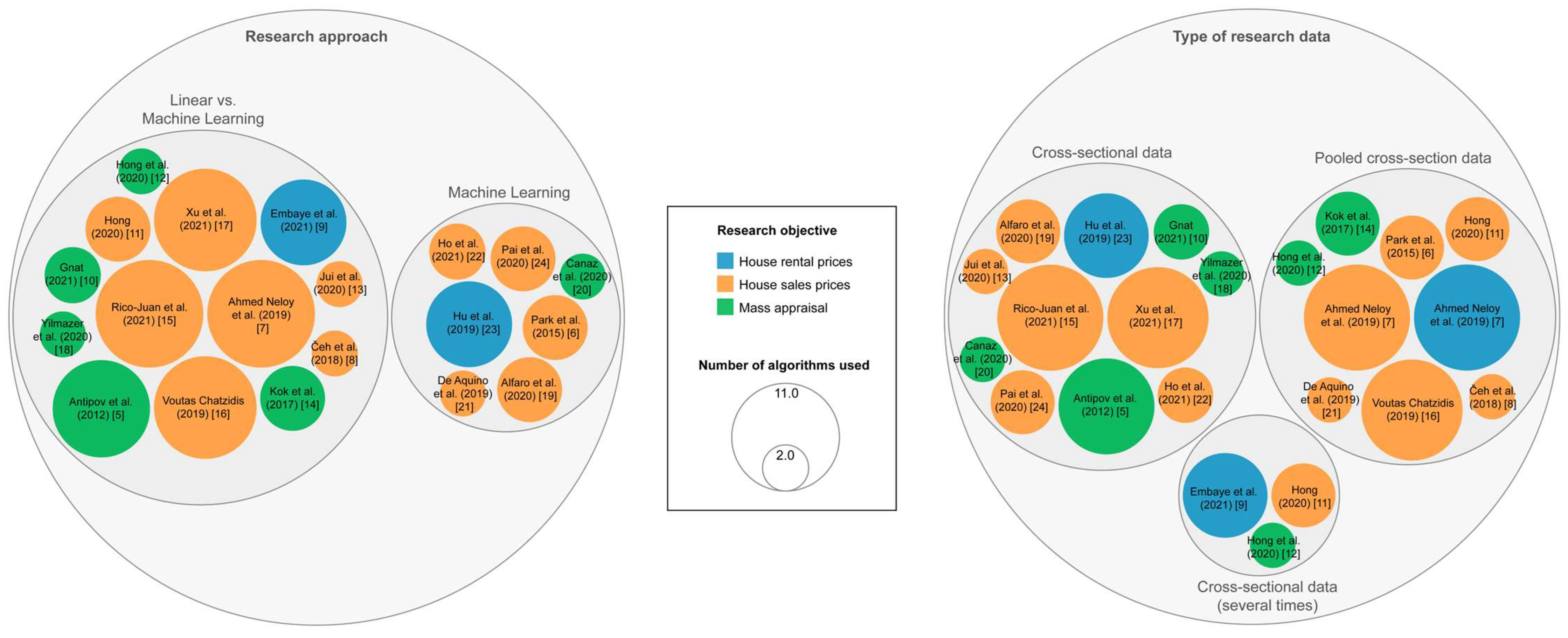
1.1. House Prices and Machine Learning

Park et al. [6] researched what ML models were most accurate in determining house prices. To this end, they used a sample of 5359 row houses in Virginia. They used two techniques; the first was to resolve a classification problem through the RF technique, and the second was to use a regression using the naïve Bayesian algorithm. The results showed that the RIPPER algorithm improved the prediction of prices significantly.
In response to the classification problem in terms of determining whether house prices would increase or decrease, Banerjee et al. [26] analyzed several machine learning algorithms. To this end, they used a dataset published on the website Kaggle.com and used different machine learning techniques such as support vector machines (SVM), neural networks (NN), and the RF technique. The results show that the RF technique was the most accurate and at the same time had the most overfitting. In contrast, the SVM technique was the most consistent and was, therefore, the most reliable.
With regard to real estate appraisals, Kok et al. [14] analyzed the performance of several machine learning techniques. They examined 84,305 observations from the states of California, Florida, and Texas, during the period from 2011 to 2016, and compared different learning techniques such as the ordinary least squares regression (OLS), RF, GBR, and XGBM techniques. The results showed that, in general terms, XGBM was the algorithm that worked best.
Čeh et al. [8] compared the RF algorithm against the hedonic price model with the purpose of analyzing which technique would obtain better predictions. The authors used a sample of 7407 properties during the period between 2008 and 2013 in Ljubljana (Slovenia). The results showed that the RF model had a better predictive performance.
In a competition organized by Kaggle.com, in which participants had to propose an algorithm for the prediction of house prices, Fan et al. [27] used predictive algorithms based on regressions such as RF, SVM (several kernels), XGBM, ridge and LASSO linear regression. The data were provided by Ames Housing in Iowa, with records from 2006 to 2010. The results showed that ridge, LASSO, and XGBM had a lower prediction error.
Hu et al. [23] analyzed predictive performance through supervised learning algorithms for housing rental prices in Shenzhen (China). The authors used RF, ETR, GBR, SVR, multi-layer perceptron neural network (MLP-NN), and k-NN algorithms. The results showed that the RF and ETR algorithms had a better predictive performance.
To predict apartment rental prices in Dhaka (Bangladesh), Ahmed Neloy et al. [7] compared several algorithms. They selected various algorithms: MLP-NN, RF, SVM, decision tree (DT), LASSO, ridge, and elastic net. The results showed that the RF algorithms had a lower mean square error.
Voutas Chatzidis [16] used different regression-based machine algorithms to predict house prices in the Netherlands. The author used LGBM, XGBM, CatBoost, and RF algorithms, with CatBoost obtaining the best results with an accuracy rate of 90%.
In a study that looked at the whole of Spain, Alfaro-Navarro et al. [19] proposed a new methodology to carry out the automated prediction of house prices. A different model was generated for each municipality and a sample of 790,631 properties for the 433 municipalities analyzed was achieved. The models were carried out using bagging, boosting, and random forest algorithms. The results show that the bagging and random forest algorithms were slightly better.
Hong [11] compared the predictive behavior of the HPM versus machine learning using three algorithms (XGBM, LGBM, CatBoost) to predict the transaction price of apartments in Seoul. To this end, the author used a sample of 620,617 observations for the period between 2009 and 2019. The results showed that ML algorithms had more predictive power than OLS. Moreover, it was noted that the CatBoost algorithm was superior in terms of predicting price even when outliers were involved. Furthermore, the ensemble model, consisting of the three algorithms, was found to have a higher accuracy than the individual algorithms.
To predict the transaction price of apartments in Gangnam (South Korea), Hong et al. [12] compared the predictive behavior of HPM against machine learning through the use of the RF technique. To this end, the authors used a sample consisting of 16,601 apartments for the period between 2006 and 2017. The results showed that the RF technique was superior in terms of predicting price.

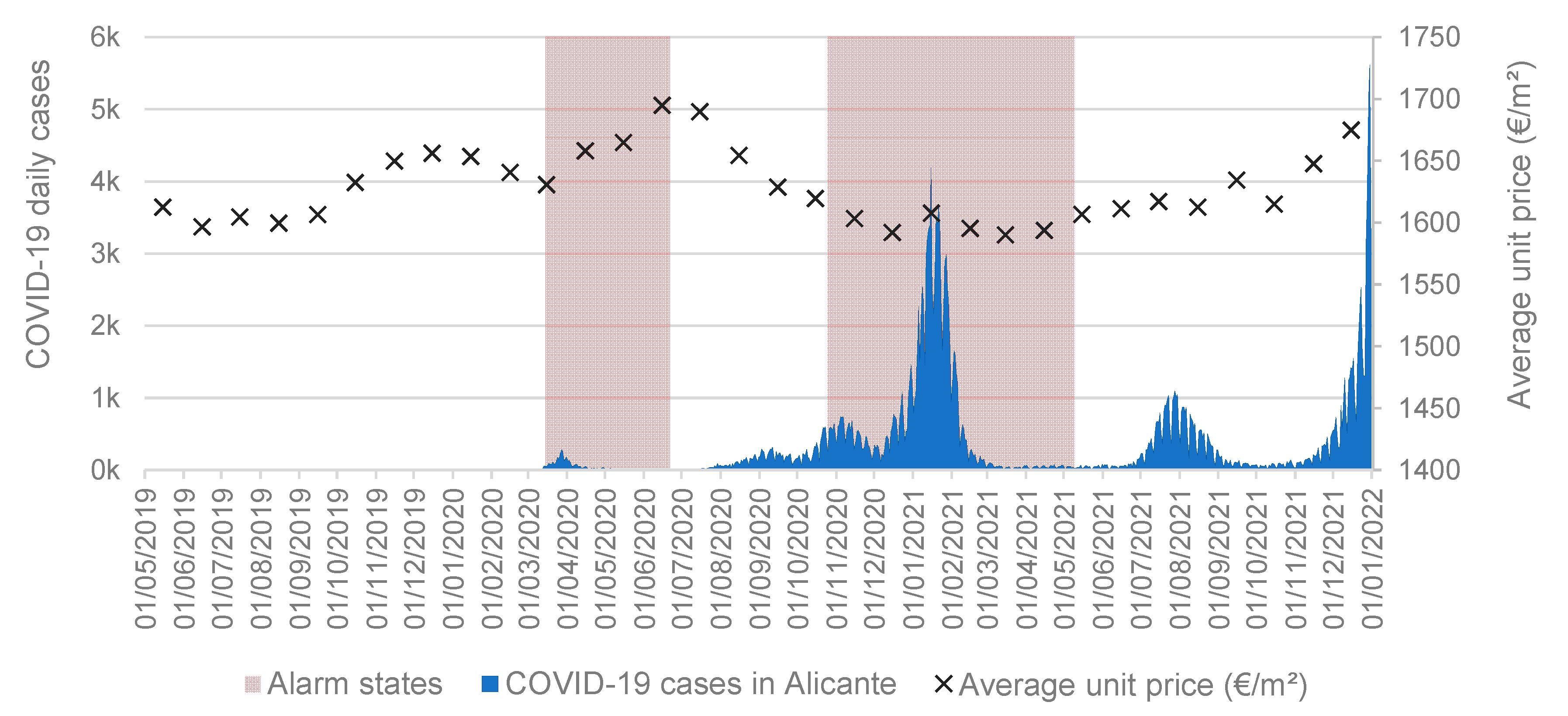
1.2. House Prices and COVID-19

The pandemic caused by COVID-19 has had a major impact in all countries, affecting all areas [28]. The real estate market has been affected over the years by various economic, environmental and health factors. This new pandemic has also had effects on the housing market.
Mohammed et al. [29] conducted a review of recent literature about the consequences of COVID-19 on the housing market, observing both negative and positive impacts on house prices, supply and demand. In some cases, there was an increase in the price and supply of housing with higher amenities or located in suburban areas. On the other hand, in other areas, house prices, supply and demand decreased for different reasons. In addition, other negative effects were identified, such as difficulties in mortgage return maintenance and the delay of new construction due to health restrictions.
Other studies have analyzed the effects of the pandemic in different regions of the world, such as the United States [30,31,32], the Eurozone [33], Spain [34], Poland [35], China [36,37,38], Australia [39] and Turkey [40,41]. The main conclusion that can be drawn from them is that the price varied differently from region to region and that consumer preferences shifted towards less densely populated areas in the periphery.
In the United States, COVID-19 caused high-income households to seek single-family homes with larger floor areas, leading to a decrease in the price of multifamily housing [32]. Other authors [30,31] observed that house prices fluctuated differently in different regions and that housing demand increased in the periphery with lower population density and in smaller cities far from urban centers with high population density.
In the Eurozone, Battistini et al. [33] described that initially there was a reduction in real estate activity as a consequence of mobility restrictions, but that it did not affect the upward trend in prices (third and fourth quarter of 2020) because of the political and fiscal measures adopted by the governments.
In Spain, Alves Álvarez et al. [34] indicated that real estate market activity was intensely reduced in the first months after the pandemic declaration, with activity recovering as restrictions were lifted. House prices showed a generalized slowdown by regions, being higher in areas of the Mediterranean coast and islands, mainly due to the reduction of foreign buyers.

2. Materials and Methods

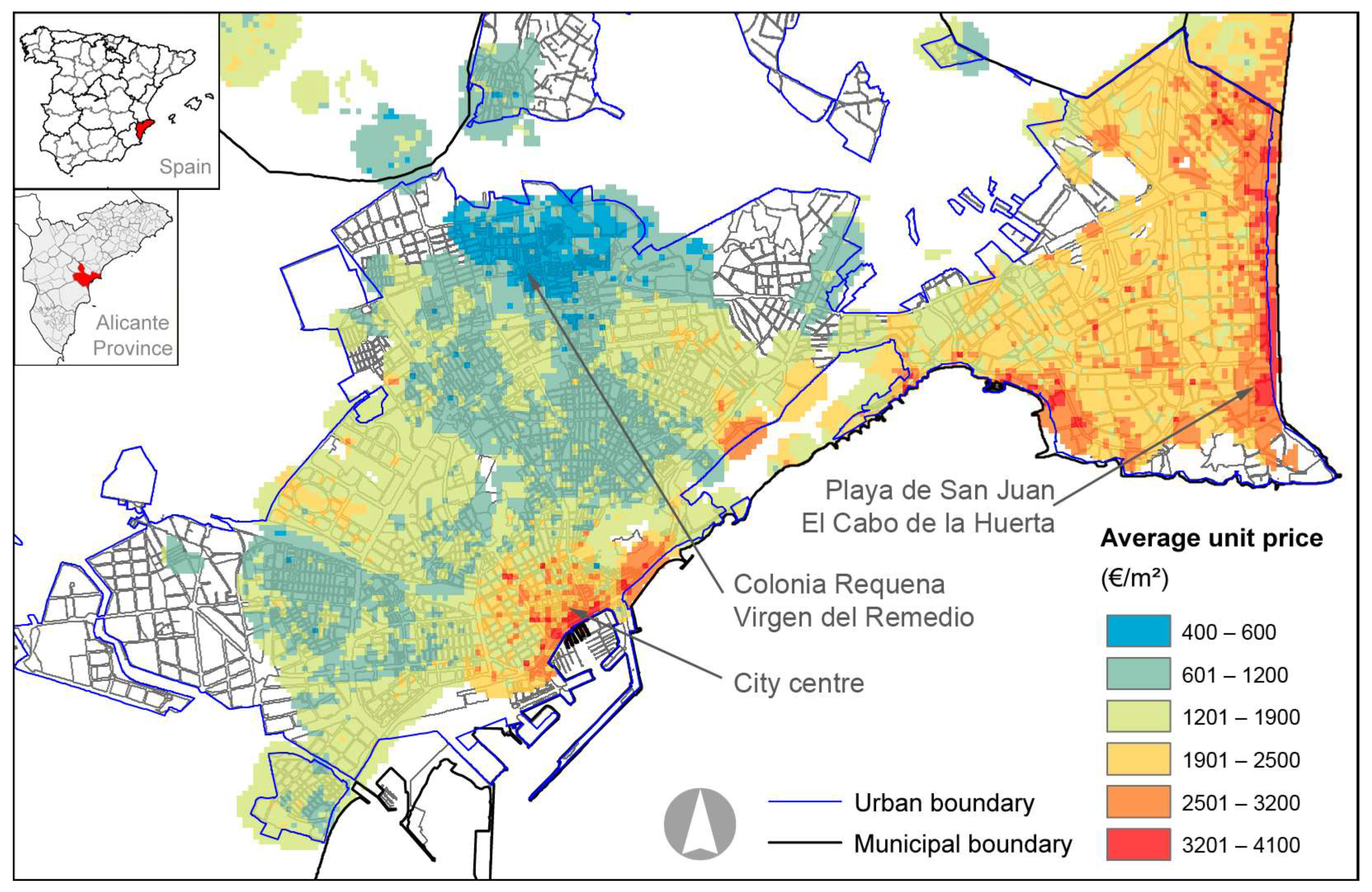
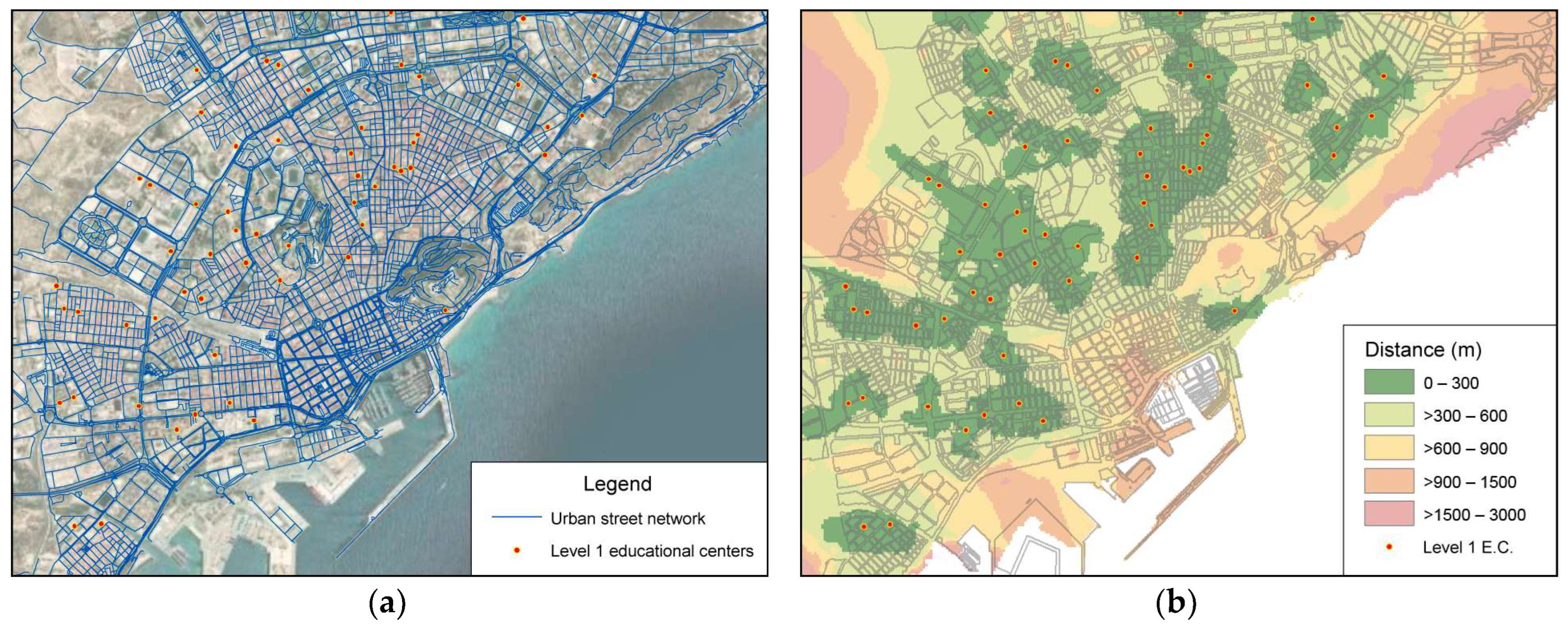
2.1. Study Area, Information Sources, and Database

The focus of this study was the city of Alicante (Valencian Community), the capital of the province, which is home to 18% of the total population of the province of Alicante. Alicante is considered one of the biggest municipalities in Spain as it ranks eleventh in terms of population [42]. Alicante is a port city on the Mediterranean coast and forms a conurbation with other neighboring municipalities. The city of Alicante is of great importance in the Spanish real estate market, since in 2021 it ranked seventh in terms of the number of real estate transactions (1% of total transactions nationwide), the main Spanish drivers being Madrid (6.6%), Barcelona (2.5%) and Valencia (1.8%) [43].
There is a large spatial difference in the distribution of house prices (Figure 2) in the city of Alicante. The area with the highest prices is located in the northeast of the municipality, in the areas of Playa de San Juan and El Cabo de la Huerta, which sit along the widest coastline of the municipality. The properties with the lowest prices are located in the north of the city, where the neighborhoods of Virgen del Remedio and Colonia Requena, among others, can be found.
The pandemic evolution derived from COVID-19 manifested itself differently in the province of Alicante compared to the national context. For each case detected in the Alicante province, 25 cases were identified in the national context. Figure 3 shows the evolution of reported cases of COVID-19 to the Red RENAVE [44] in the province of Alicante (left vertical axis), and the average monthly multifamily housing unit prices in the city of Alicante (right vertical axis). In the last quarter of 2019, there was an upward trend in prices, shifting to a downward trend during the first quarter of 2020. During the second quarter of 2020, coinciding with the first alarm state, there was an upward trend in prices, reaching a peak in June 2020. In the third and fourth quarters of 2020, there was a decline in the average house price, with a 6.1% reduction in December 2020 compared to June 2020. It is from May 2021, coinciding with the end of the second alarm state, when a slight upward trend in prices began.
In Spain, there are no official sources with open and public data on transaction prices, so it is common in these cases to use price lists from real estate portals. Several authors suggest that real estate asking prices can be an adequate substitute for transaction prices [45,46,47,48]. For this reason, it should be taken into account that the results of this research are based on asking prices, so they may not necessarily reflect the behavior of transaction prices.
The information regarding the listing prices was taken from a real estate website, with the asking prices and features of both properties and buildings being collected. Data about the listing prices, the features of the property (type, floor area, number of bedrooms, bathrooms, etc.), the features of the building (elevator, parking space, swimming pool, etc.), and spatial location (geographic coordinates) were collected.
From May 2019 to December 2021, around 49,875 different multifamily properties offered for sale were collected from a real estate portal. Each month, a search was carried out to identify whether there were new listing prices that had not been identified in previous months, to verify whether the existing properties were still for sale or whether the price had changed, and to omit the properties that were no longer found. By doing this, it was possible to document, for each property, the period that it was offered on the market as well as the changes in price over time (monthly changes).
The information given by those advertising properties was sometimes incomplete or incorrect, which led to data inconsistencies that needed to be reviewed. Unlikely values were identified in several of the quantitative features, such as the size of the property, the number of bedrooms, and the prices. To identify the values, a univariate outlier analysis was carried out and those properties with values greater or less than six standard deviations in all quantitative characteristics (area, number of bedrooms, and number of bathrooms/toilets) were discarded. Once the database had been revised, those cases in which data was missing for some relevant features were excluded; this included properties with no price given, properties without location coordinates, and properties that did not have their floor area and number of bedrooms or bathrooms/toilets listed. After the process of data cleansing had been completed, 2506 properties were discarded, leaving 47,369 different properties for the sample.
As it is common for identical properties to be marketed in the same building, a second data cleansing process was carried out, which consisted of identifying and eliminating datasets for properties that had identical features. This was done with the purpose of avoiding data leakage between different subsets of data used in the subsequent analyses (training/validation/test). In this process, 7426 properties were discarded from the sample, leaving a final sample that consisted of 39,943 different properties, which is 80.1% of the initial sample.
The information provided by the real estate portal was georeferenced in a geographic information system in order to create new features in the dataset. Kok et al. [14] consider it to be particularly important to include information about the local neighborhood that complements the usual features used in house price estimates. Other sources of information were used to create these new features, such as the Spanish National Statistics Institute (INE), the General Directorate of Cadastre (DGC), the National Geographic Institute (IGN), the Regional Ministry of Education, Culture and Sport (CECD), the Valencian Cartographic Institute (ICV), and the U.S. Geological Survey (USGS).
Using the mapping of the census tract [49] and the census of the population by municipality [42] obtained from the Spanish National Statistics Institute, population data regarding the dependency ratio, the aging ratio, and the percentage of foreign population corresponding to the year 2020 were extracted. Using the Atlas of Household Income Distribution [50], an experimental statistic prepared by the INE, data regarding the net income per household at the census tract level for the year 2019 (latest published statistic) were extracted. All these features were calculated with data at the census tract level, in order to ensure that all properties in the same census tract would have the same values.
Using the alphanumeric and vector information from the General Directorate for Cadastre [51], and following the methodology developed by [52] for the processing of cadastral data, a raster map was created, which detailed the average age of the environment surrounding the properties and gave a ratio of the built-up area in the vicinity of each building (150 m around the building).
To calculate the distances, the transport network prepared by the Spanish National Geographic Institute [53], the location of the educational centers of the Regional Ministry of Education, Culture and Sport [54], and the mapping of green areas obtained from the Valencian Cartographic Institute [55], were all used. With this spatial information, the distances between properties and public services (namely the distances from the educational centers, green areas, and the coast) were calculated. The distances were calculated by network, that is, using the distance between the origin and destination through a pre-established layout of streets and crossroads, which simulates the reality of the urban network (see Figure 4) [56]. The Network Analyst extension of ArcMap 10.3 was used, calculating the distance by network from each property to each point of interest. The network was modeled with street sections and the nodes or intersections, also simulating the presence of bridges or tunnels. Distances between an origin (or a destination) and the network were calculated as the minimum distance from the origin/destination to the network.
To calculate the normalized difference vegetation index (NDVI), the multispectral satellite images from the USGS [57] were used. Images provided by the satellite Landsat 8 in 2020 with path 199 and row 033 and low cloud cover (<20%) were selected. These images corresponded to three different dates in an entire year and were selected to observe any variations between seasons (March, July, December). With the three rasters, and through the use of map algebra, a raster with average values for an area of influence measuring 150 m was calculated. Each property was assigned an NDVI value using a spatial overlap analysis.
The Raster Calculator and Focal Statistics tools of the Spatial Analyst extension of ArcMap 10.3 were used to calculate the NDVI (feature D_NDVI_150m) (see Figure 5). The NDVI was calculated with the Raster Calculator and the rasters of the red and near-infrared bands of the three selected days of the year 2020, then the average of the three rasters was calculated. Using the Focal Statistics analysis, the average in an area of influence of 150 m (circle neighborhood) was calculated for each pixel. Using the Extract Raster Values to Point tool, the average NDVI value in the surrounding area was assigned to each property.
Finally, to model the effect of time, a feature was created with different categories that identified whether a particular property was being marketed in a given quarter. The process of data appending for the temporal data is detailed in Figure 6, which shows that a property can appear many times in a temporal dataset, depending on the quarter in which it was marketed. This new pooled cross-sectional dataset was formed by 94,024 records, corresponding to 39,943 different properties offered between May 2019 and December 2021.
Table 1 presents the 28 features constructed from the data obtained for this research, which are arranged according to five categories: Dwelling characteristics (A), Building characteristics (B), Location characteristics (C), Neighborhood characteristics (D), and Temporal characteristics (E). The unit with which each variable has been measured is also indicated, as well as a brief description of the same.
The selection of the features used was based on the literature review of other research, the availability of data and the previous experience of other research conducted in the Alicante real estate market [58,59,60,61].
In addition to the features mentioned, the data obtained from the real estate web portal allowed for the creation of other features (floor, balcony availability, sports facilities, marketer, etc.). However, these features were not included in Table 1 and were not used in the research, since they were discarded in the feature engineering phase for having little variability or a large number of missing values.

2.2. Descriptive Statistics
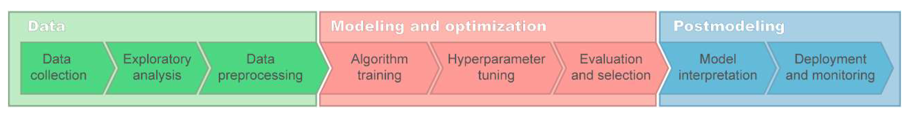
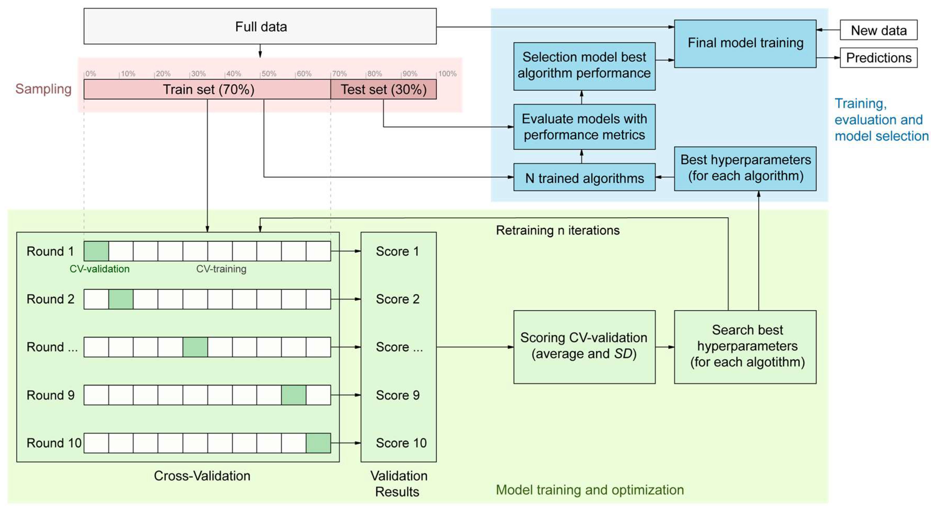
Table 2 shows the descriptive statistics for all features used in the analysis.
Figure 7 shows the distribution of the unit price (€/m²) for each of the quarters analyzed. As can be noted, the price distribution over the quarters was very uniform, with variations only being small. Specifically, the number of properties offered with prices exceeding 1700 €/m² reduced over time, with there having been more properties in the 900–1100 €/m² price range in the last quarter of the analyzed series.
Figure 8 shows the distribution of the unit price according to whether the properties had an elevator. It can be noted that when an elevator is available, price distribution is displaced and extends further in areas with higher prices than in the sample without elevators. In the case of properties without elevators, prices are more concentrated and are found in lower-priced areas.

2.3. Methodology

In this study, 5 machine learning algorithms were used to develop a house price prediction model for a case study with the city of Alicante. To this end, all the steps expected in the usual machine learning workflow were addressed (Figure 9): data preparation, feature engineering, hyperparameter training and optimization, model evaluation and selection, and, finally, model interpretation.
The Python (3.7.11) programming language was used and the pandas (1.3.2) and numpy (1.19.5) libraries were used for data processing. To implement the ML algorithms, machine learning libraries scikit-learn (0.23.2) with scikit-optimize (0.8.1) and pycaret (2.3.2), as well as the lightgbm (3.2.1) and xgboost (1.4.2) libraries, were used. To create the graphs, the matplotlib (3.4.2), seaborn (0.11.2), and yellowbrick (1.3. post1) libraries were used. The interpretation of the model was implemented with scikit-learn (0.23.2) and eli5 (0.11.0). Table 3 details the 6 algorithms used, indicating the origin of the library.
Data collection was carried out using web scraping through a specific program developed by the authors. The structured information was stored in a database that could be exported to other exchange formats. The previous exploratory analysis of the data allowed for the preprocessing phase. During the preprocessing phase, outliers were identified, data were cleaned, missing data were treated and unrepresentative categorical variables were pooled together, as described in Section 2.1. Finally, the dependent variable (house prices) was transformed into the natural logarithm. The logarithmic transformation reduced problems of heteroscedasticity and improved the goodness-of-fit of the data [45,62,63]. Moreover, the transformation facilitated the interpretation of the coefficients since they show the percentage of variation in the dependent variable that would be obtained for each one-unit increase in the explanatory variable [62].
In the feature engineering phase, the correlations between features were analyzed and some features were eliminated due to their high correlation. For this analysis of the collinearity of the features, the variance inflation factor (VIF) was used, regarding which many authors have suggested that there are collinearity problems if a VIF is higher than 10 [64,65]. Some features were also discarded for having low variance and others were discarded for having a high percentage of missing values. It was not necessary to carry out a process for the creation or extraction of new features.
For the development of the training and evaluation phases for the models, it was necessary to divide the dataset (Figure 10). All divisions were carried out with the purpose of separating datasets according to a group identifier (“GroupShuffleSplit” from the scikit-learn library), with the property identifier being the attribute used to establish the groups. In this way, the different prices for the property could only be assigned to a single dataset division, thus avoiding data leakage between the training and test sets.
Two divisions were made with the full dataset, one division was for training and the search for hyperparameters (70%) and the other was for carrying out tests (30%).
In the model training phase, different potential algorithms were used to estimate their predictive power. To evaluate the performance of the models, several error metrics (mean absolute error—MAE, mean square error—MSE, root mean squared error—RMSE) and goodness-of-fit (R² score) were used. This training phase was repeated for each combination of hyperparameters created in the following optimization phase.
Hyperparameter optimization was done with the intention of improving the goodness-of-fit of the models and minimizing prediction errors. Through the selection of algorithms, the incidence of their hyperparameters was evaluated and they were adjusted by means of cross-validation techniques on the training set. In the training set, a strategy using k-fold cross-validation based on non-overlapping groups (“GroupKFold” from the scikit-learn library) with 10 folds was used, allowing a performance metric of the trained model to be obtained [66]. The cross-validation process consisted of extracting a subset of data formed by k-1 folds that was used to train the model (CV-training), and the subset formed by the excluded fold was used to estimate the performance (CV-validation). The process was repeated k times and excluded a different fold each time, quantifying the performance in all the k rounds. The average value of the scores obtained for all of the rounds and the standard deviation were used as metrics to identify the best hyperparameters and classify the algorithms according to their performance (Figure 10). The search for hyperparameters was carried out using two different algorithms; a random search and a Bayesian search. In these training and optimization phases, it was particularly important to separate the rows according to the group in order to avoid data leakage between the CV-validation and CV-training sets.
For the model evaluation process, the test datasets, and the algorithms and the hyperparameters obtained in the previous phase were used. Performance metrics and graphical techniques for prediction visualization, such as residual plots, were used to evaluate prediction errors. Moreover, the possible existence of overfitting was studied through the use of the learning curves obtained by cross-validation. The model selection process was carried out using the performance metrics (error and goodness-of-fit) obtained from the test dataset with the purpose of identifying the algorithm that performed best in predicting the dependent variable.
For the model interpretation process, tools were used to identify the most important features through the use of global approaches; namely, the permutation importance and the partial dependence plot (PDP).
For the deployment of the final model, once the most suitable algorithms and hyperparameters had been chosen, the algorithms were trained using all available data, and performance metrics were extracted.
The workflow would conclude with the deployment of the model and its monitoring. In this phase, it would be usual to develop a web platform to put the model into production, allowing predictions to be made from initial data, monitoring the model over time.

3. Results

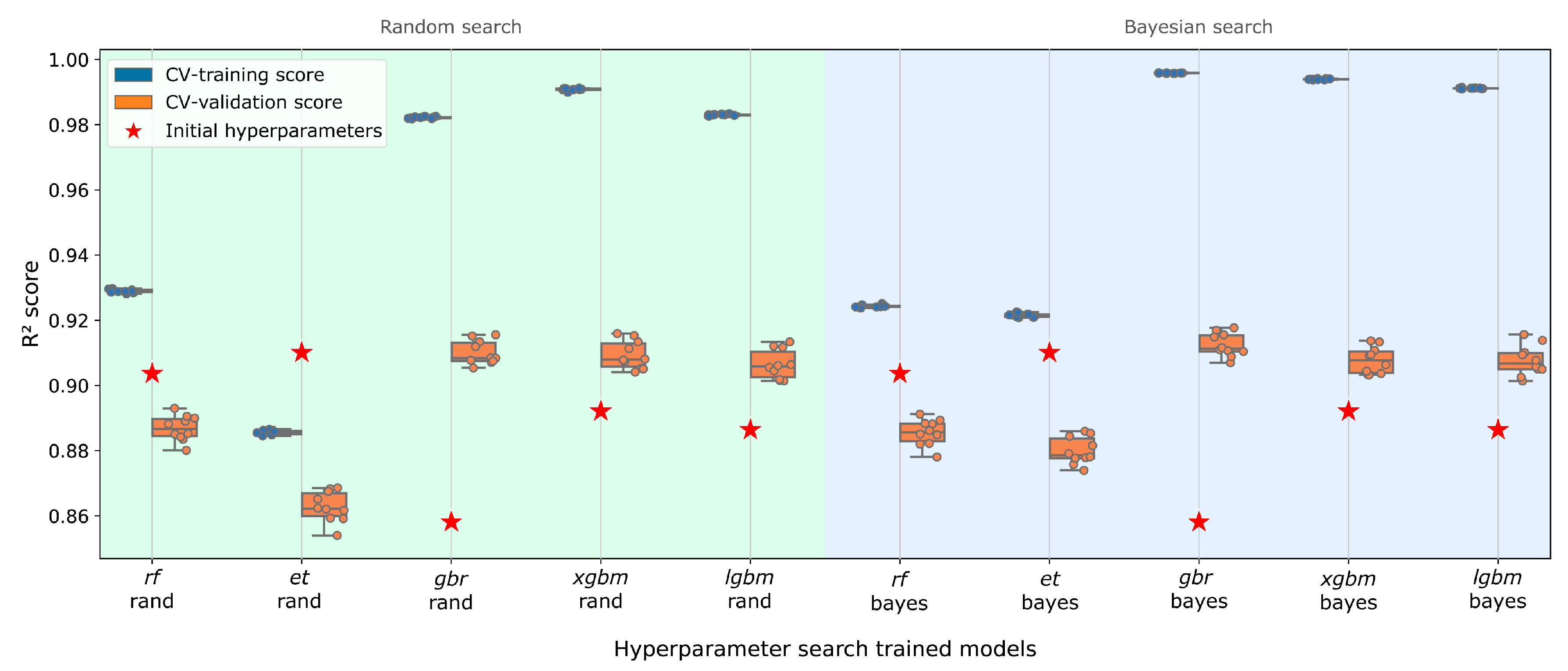
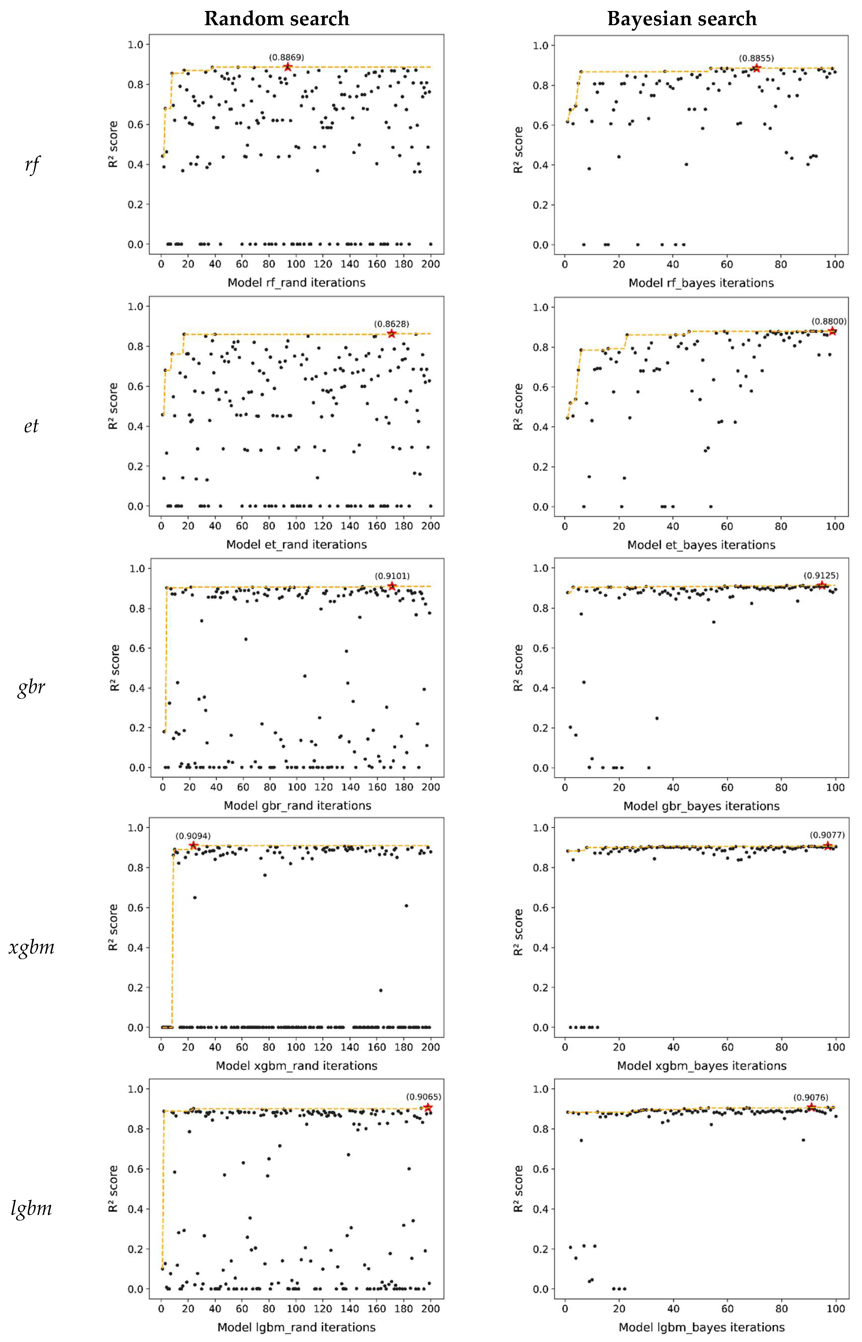
3.1. Model Training and Optimization

In the feature engineering phase, correlated features that caused multicollinearity were identified and were eliminated from the dataset accordingly. The number of bedrooms (A_bedrooms) shows a high positive correlation with the properties’ floor area. The garden feature (B_garden) is positively correlated with having a pool. The aging ratio (D_elderly) is correlated with the dependency ratio, with the latter remaining in the model. The floor area ratio (D_FAR) is positively correlated with the NDVI, the X and Y coordinates, and having a pool, and is negatively correlated with the average age of the neighborhood. Finally, regarding distances, the distance to level 2 educational centers (D_d_educ2_km) is positively correlated with the distance to level 1 educational centers and the distance to the coast (D_d_coast_km) is positively correlated with coordinate x. For the other features, the VIF was calculated and there were no values over 3.2.
Once the dataset and the training pipeline had been prepared, the models were trained with the hyperparameters preconfigured in the algorithms. Each algorithm was then trained using a randomized search (with 200 iterations) and a Bayesian search (with 100 iterations). Table 4 shows the results from the training and optimization of the ML algorithms together with the results of an ordinary least squares regression model that was used as a baseline to be exceeded. Figure 11 shows a box diagram of all the algorithms and the two types of hyperparameter searches, showing the CV-training, CV-validation, and initial model performance values.
The best hyperparameter search results were achieved with the gbr, xgbm and lgbm algorithms, especially with the gbr algorithm since it has gone from being the worst in terms of performance to being the best, with an improvement in R² score of 6.3%. The rf and et algorithms showed no improvement with regard to the performance obtained with the initial preconfigured hyperparameters.
Figure 12 shows the learning curves for the hyperparameter search. The first conclusion that can be made is that a Bayesian hyperparameter search obtains better results than a random search in fewer iterations. In a random search, many inefficient hyperparameter combinations are generated.

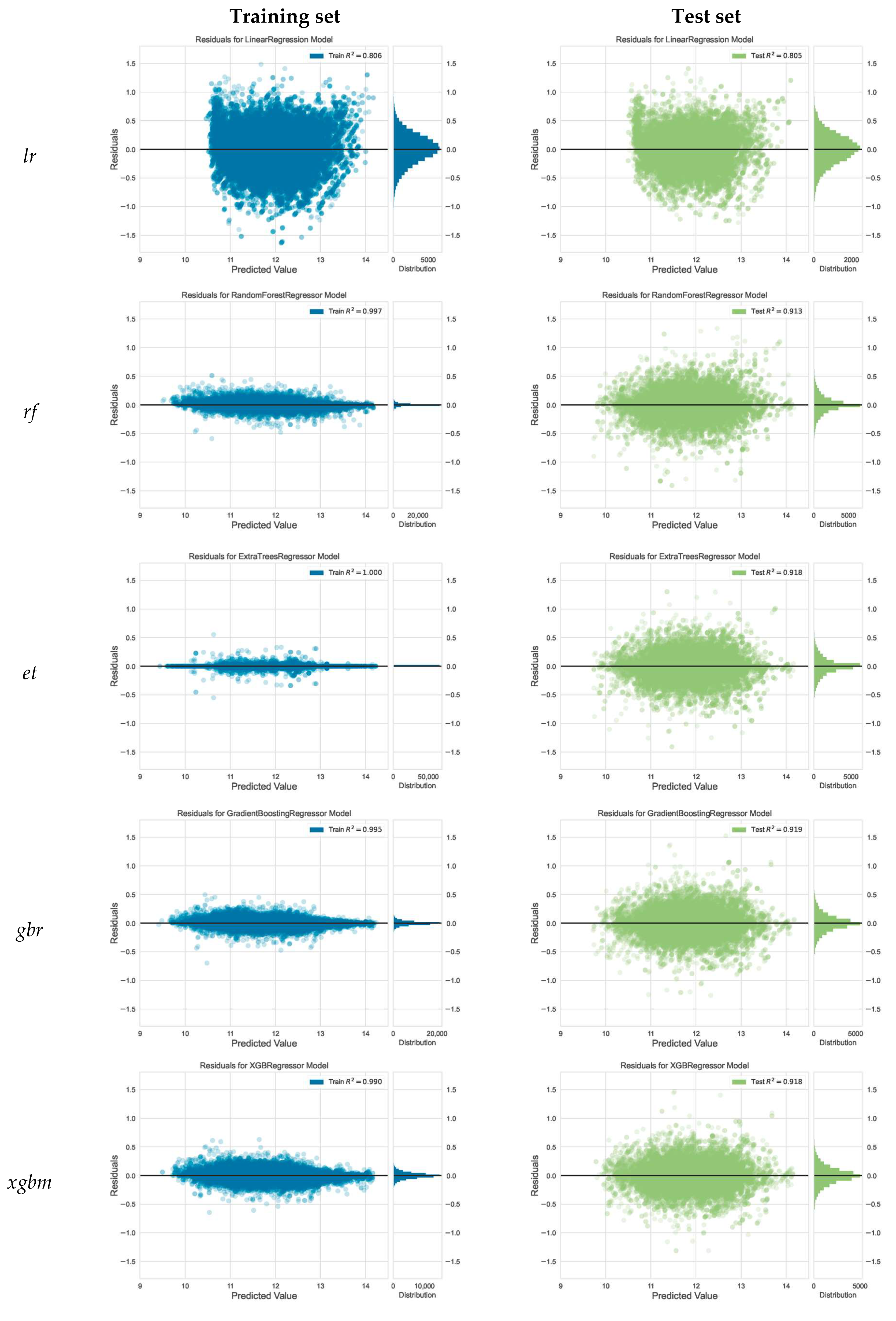
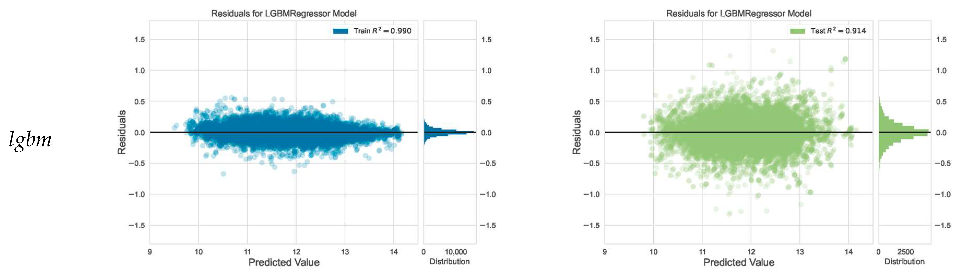
3.2. Model Evaluation and Selection

Using the trained models with the best hyperparameters, performance metrics were extracted for the training and test sets (Table 5). The values in the CV-validation column correspond with the performance metrics from the best models (see Table 4) and are replicated in this table for information and comparison purposes only. The overfitting column was calculated as the percentage difference between the test set and the training set. Figure 13 shows the residual plots from the trained algorithms and divides the training and test sets.
The results show that the rf and et algorithms are those with the most overfitting (close to 9%), while the xgbm algorithm has the least overfitting, with there being a difference of +7.9% between the test set and the training set. This can also be seen in the residual graphs for the rf and et algorithms (Figure 13), in which the point cloud for the training set errors is particularly concentrated on the 0 standard deviations line, while the point cloud for the test set errors is more dispersed. The results are stable and consistent since the difference between the performances (R² score) of the test sets and those obtained in the cross validation (CV-validation) are very low, between 0.00–0.01.
Figure 14 shows the learning curves for the algorithms and the time taken for their training for different sample sizes. For the rf and et models, an almost perfect overfitting can be noted in the training set, which does not vary with the increase of the sample size, thus indicating an excessive overfitting of these algorithms. With the xgbm and lgbm algorithms it can be observed that, as the size of the dataset increases (higher complexity), the accuracy in the training set decreases, thus reducing overfitting. These results suggest that the algorithms based on bagging tend to overfit the training data more than algorithms based on boosting.
Regarding the time taken in training according to the size of the dataset, it can be observed that the xgbm and lgbm algorithms are the quickest; and gbr is the fastest for small datasets. The rf and et algorithms can result in being prohibitive as the size of the dataset increases.
To evaluate the final performance of the models, the algorithms were trained again with the best hyperparameters using the entire dataset (training and test) and their new performances were calculated. The results are shown in Table 6.
At this stage, it is possible to select the most efficient algorithm, or algorithms, to predict the house prices in the city of Alicante. A simple option would be to choose the algorithm with the best performance in the test dataset (Table 5), without considering other aspects. In this case, the gbr algorithm would be chosen as it also obtained the best performance in the cross-validation process. However, the choice is not that simple as other aspects must be considered, such as:
  • The difference in performance between the algorithms (in this case being minimal, varying between 0.9135 and 0.9192 (R² score));
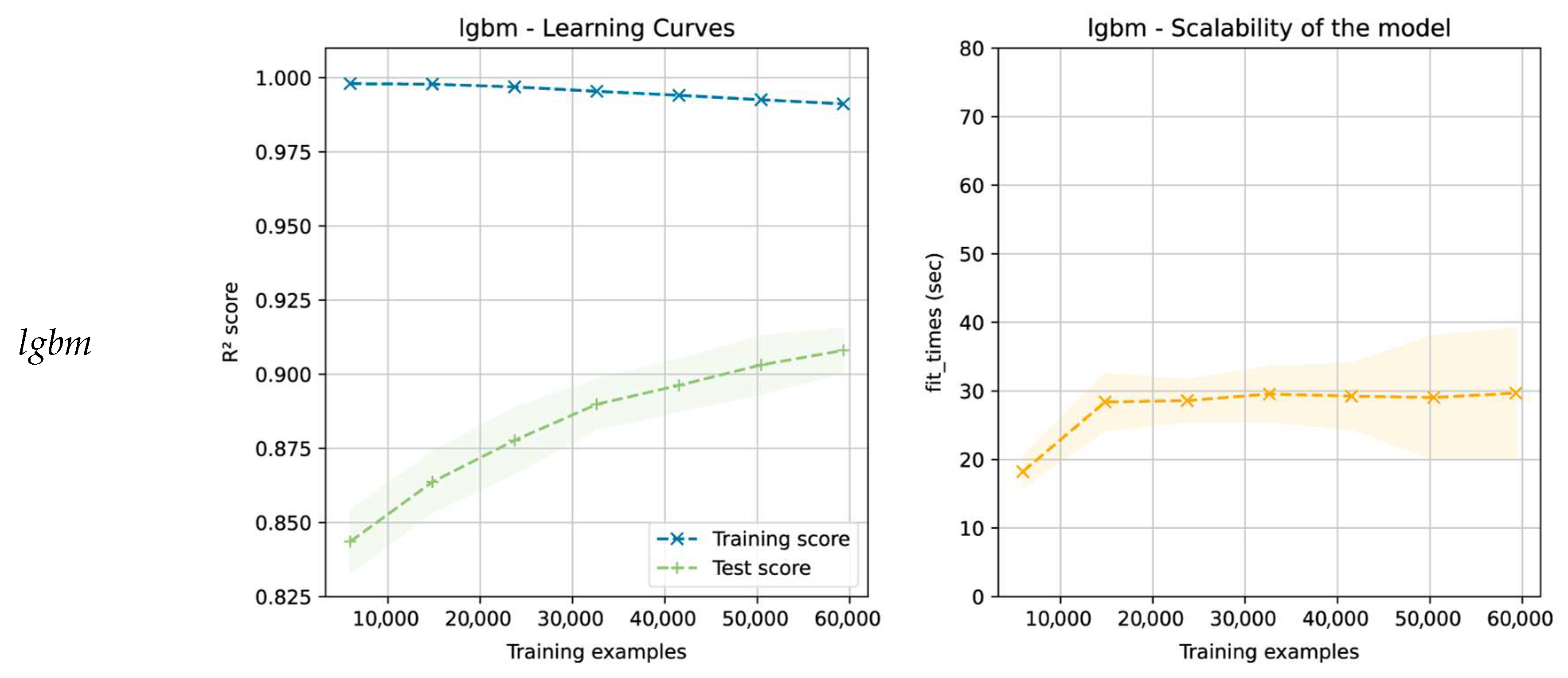
  • The need to select an algorithm that has no overfitting problems and generalizes well with unseen data (in this case, the xgbm and lgbm algorithms may be good candidates);
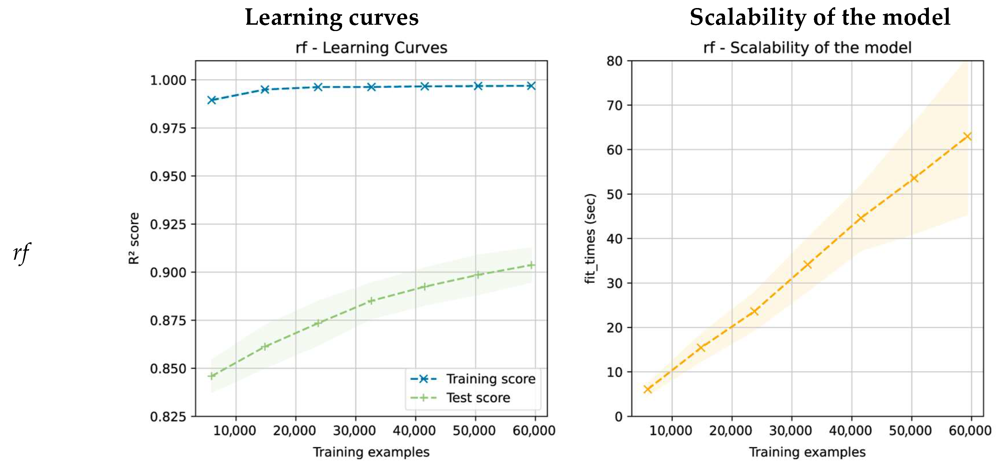
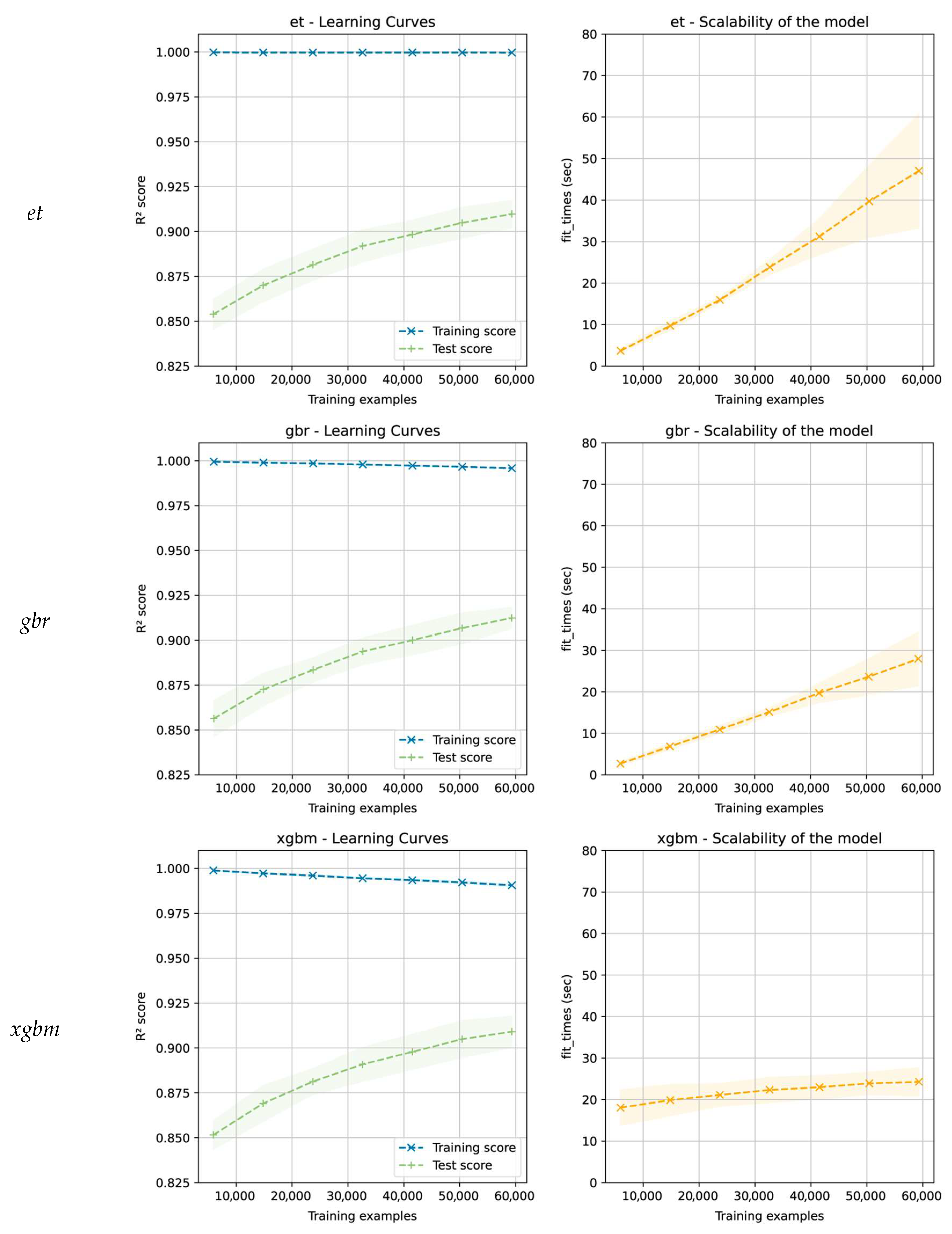
  • The need to choose an algorithm with low prediction variability in the cross-validation process (low variance) (the gbr algorithm has had the lowest variability);
  • The need to consider the necessary times for the training and optimization of the hyperparameters and whether they adapt to the project deadlines (in this case, the xgbm and lgbm algorithms are the best options);
  • The need to consider the file sizes of the models required for deployment (in this case, the lgbm algorithm generates the smallest file and the rf and et algorithms generate the largest (77 to 112 times larger than the lgbm algorithm)).
The performance, existence of overfitting, and training time will vary depending on the combination of hyperparameters used, so it is difficult to generalize the best algorithm. For this reason, it is necessary to test a set of algorithms with different combinations of hyperparameters and evaluate their results.

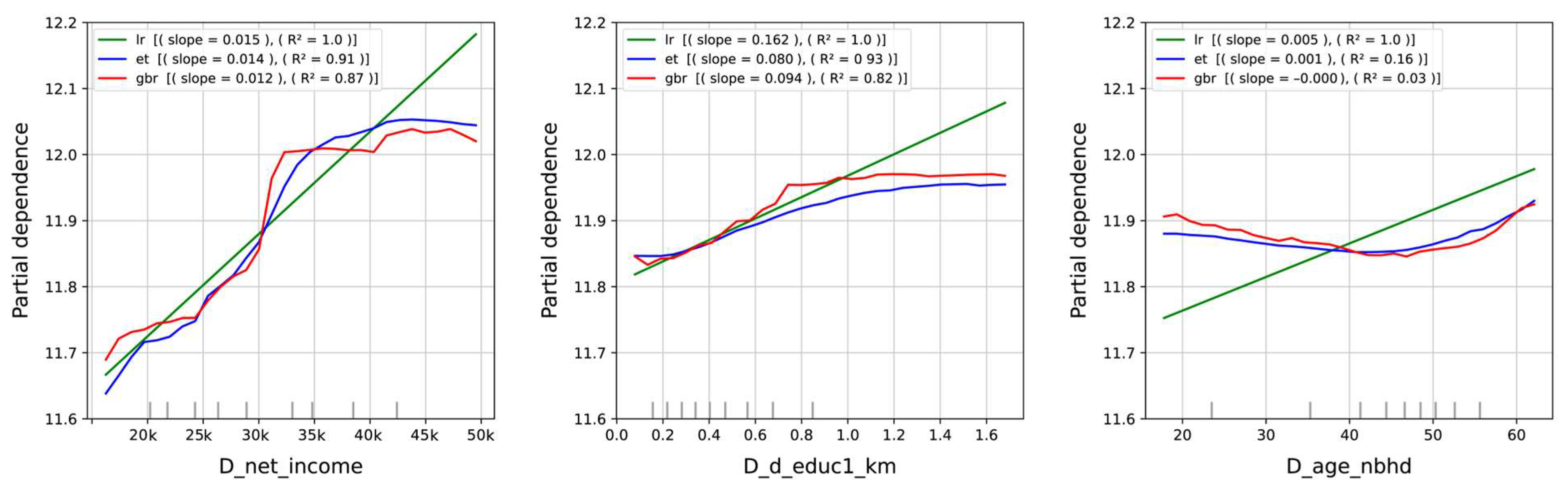
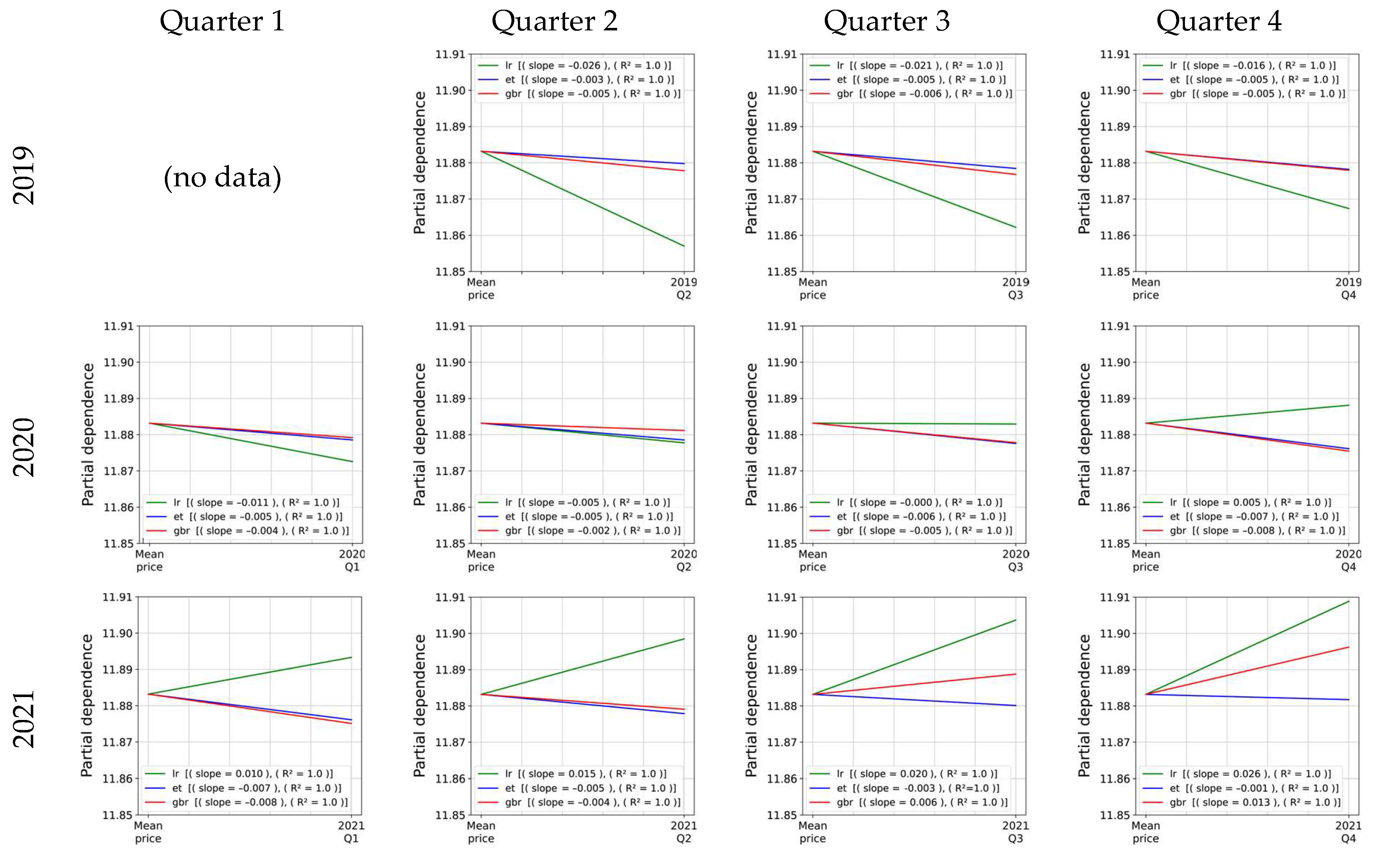
3.3. Model Interpretation

There is a wide collection of libraries dedicated to the interpretation of ML algorithms [67]. In this case, two global strategies were used; the relative importance of features by means of permutation and partial dependence plots.
The large majority of ML algorithms are able to calculate a measure of relative importance of features and identify those that are more relevant for the prediction of the dependent variable. These metrics used in the algorithms do not allow for their comparison since they are calculated with different strategies. In linear regression, the importance of the features is determined by the standardized regression coefficients, which are obtained after standardizing the original features introduced into the model.
A strategy called permutation importance, which was implemented in the ELI5 library [68,69], was used to calculate the importance of a feature when it was not in the model using performance metrics.
Using this strategy has several advantages: (1) the strategy is agnostic and is, therefore, independent from the model, meaning it can be used with any algorithm; (2) the metric obtained is easy to interpret and allows for the comparison of results between different algorithms. In this case, the R² was used, which is interpreted as the reduction in the percentage of variance that would occur in the model by removing the corresponding feature; and (3) it is much more computationally lightweight than other strategies (see [70,71]) since it does not require more models with other feature combinations to be trained.
The permutation importance process is as follows: (1) for each feature, the dataset values are shuffled (introducing random noise) in order to maintain the statistics of each feature (mean, SD, min, max); (2) the predictions are extracted using the trained model and the dataset that was shuffled in the previous step; (3) the decrease in performance (R²) is calculated with regard to the performance obtained before shuffling the data; and (4) the shuffling process is repeated as many times as necessary and for each of the features.
Figure 15 shows the most important features for the prediction of house prices using the permutation importance when applied to two algorithms based on different strategies, et and gbr. The location features (C_coor_X_km and C_coor_Y_km) are relevant in both algorithms. The most important features of the properties are the floor area, the number of bathrooms, and the availability of an elevator (A_area_m2, A_bathrooms and B_elevator). Regarding the neighborhood features, the most relevant are the net household income, the distance from the property to level 1 educational centers, and the average age of the neighbourhood (D_net_income, D_d_educ1_km and D_age_nbhd).
Through the use of partial dependence plots (PDP), it is possible to visualize the marginal effect that a feature (or two) has on the predicted result of a machine learning model [72]. This type of graph can show whether the relationship between a dependent variable and an independent variable is linear, monotonic, or more complex [73]. This technique implies that the feature for which the PDP is calculated is not correlated with other model features since, in the case of high correlation, the interpretation of the PDP may be erroneous [73]. Care must be taken also in the interpretation of the graphs in the extreme areas where there are few observations.
For the purpose of comparison, the partial dependence plots for the lr, et and gbr algorithms are provided and show the feature to be analyzed on the horizontal axis and the house price (in natural logarithm) on the vertical axis. Serving as complementary information, and being used only for illustrative purposes, the slope of the lines with the best fit for each partial dependence estimate and the coefficient of determination of the fit are provided. In the case of linear regression, these graphs are shown as a linear relationship, that is, as an average rate of change. The greater the magnitude of the slope, the steeper the line and the greater the rate of change. Regarding the interior marks on the axes, they represent the distribution of the sample in deciles (represented in gray). In order to avoid misinterpretations of the extreme ends of the data distribution, the sample has been trimmed by 5% (2.5% at each extreme).
Figure 16 summarizes the PDP graphs for the location features (C_coor_X_km and C_coor_Y_km). It can be noted that house prices are higher when the property is located further east and are lower when it is located further north. The et and gbr algorithms show more complex relationships than the lr algorithm but do have the same trend (Figure 16a). It can also be noted that the trend in the Y coordinate is not uniform in all the data distribution since the lr model overestimates the effect in observations below the 30th percentile and above the 90th percentile.
For a better understanding of the relationships between these two features, a two-way directional partial dependence plots can be used. By combining the X and Y coordinates in the graph, a continuous map showing the average value of a house depending on its location can be displayed (Figure 16b). The graph does not trim the areas with no data, meaning that its interpretation should be done with caution.
The partial dependence plots for the most important property features are shown in Figure 17. Floor area and the availability of an elevator show the same trend in all three algorithms. Regarding floor area, it must be considered that the graph is cut off at 210 m², which leaves larger properties in that 2.5% of extreme cases that can distort the representation. Regarding bathrooms, it can be noted that the lr model does not predict correctly when there are more than two complete bathrooms. In this case, the et and gbr algorithms interpret that having more than two bathrooms does not affect the price (slope close to zero).
Regarding the three most important features of the neighborhood (Figure 18), it can be noted that linearity is broken in some areas of the data distribution. In the case of net household income, with values over 35 k euros, the positive slope with respect to the price is broken and has an almost null slope. A similar situation occurs with the distance to level 1 educational centers as once the distance exceeds 1000 m, the slope tends to zero. In the case of age, two different slopes can be noted; a negative slope for properties that are 0–45 years old, and a positive slope for older properties.
The temporal feature is shown in Figure 19, where each graph represents the partial dependence concerning the average price of the entire dataset [73]. By using the logarithmic transformation of the independent variable (price), the slopes of the straight lines can be interpreted as the percentage variation in price when classifying a certain category of the temporal feature (quarters), keeping the rest of the independent features constant.
It can be noted that the linear regression overestimates the impact of temporal feature, while et underestimates it. When observing the gbr lines, it can be identified that between the second quarter of 2019 and the second quarter of 2020 prices were below average, and there was an increase in prices from the third quarter of 2020 (with respect to the average price).
To complement the results of the ML models used in the research, a table with the regression coefficients and the statistics of the least squares regression model, with in-dependent results for the training and test set, is included in Appendix A (Table A1).

4. Discussion

All the machine learning algorithms performed better than the linear model based on ordinary least squares. One of the main problems of the linear models is adopting this linearity for the entire distribution of the data. This issue is partially resolved through the use of ML algorithms, since they are able to model nonlinear behaviors in heterogeneous data, such as those of the real estate market. Authors such as [11,14,15,23] have also arrived at this same conclusion. The results in Section 3.3 show examples of features with nonlinear relationships with house prices such as location (see the Y-coordinate in Figure 16a), number of bathrooms (Figure 17), and some neighborhood features (Figure 18).
The ensemble learning algorithms based on boosting (gbr, xgbm and lgbm) have shown the best behavior in various aspects, since they perform well and overfitting affects them less than other algorithms such as rf and et. The fastest algorithms are xgbm and lgbm, especially with large datasets, which may be an important factor in the training and hyperparameter optimization phases, especially for ML project developments being carried out in the business sector. The ensemble algorithms based on bagging (rf and et) have also proven to perform well; however, more overfitting is shown in the training data, which may reduce the generalization to unseen data. Overfitting is due to a higher complexity of the model, which may suffer from a higher variance in the predictions [14]. The literature review shows that there is a preference for the random forest algorithm over other types, however, in the majority of cases the existence of overfitting is not analyzed. Other authors do not limit themselves to the random forest algorithm and explore the performance of other algorithms with good results such as extra-trees regressor, Gradient Boosting Regressor, Extreme Gradient Boosting, Light Gradient Boosting Machine, and CatBoost [11,14,19,23].
Regarding the interpretation of the model, global strategies were used to identify the features that are the most relevant in the prediction of house prices. The metrics based on permutation importance have many advantages and allow for the comparison of different algorithms, favoring decision making in the selection of the features and algorithms to be used. Moreover, the partial dependence plots allow us to describe the behavior of the features and how they affect the price prediction, and also allow us to identify interactions and (non) linearities between features. Although the partial dependence plots have a more qualitative interpretation (trends, patterns, (non) linearity, and direction), they can also be interpreted quantitatively with certain precautions and limitations, just as in the traditional linear models. This phase of interpretation of the models is fundamental for the evaluation of how the algorithms behave and whether their predictions are consistent or whether there is some type of training error or error in the data itself.
In the interpretation of the models in this case study, it is identified that the most important features for the prediction of house prices are floor area, the number of bathrooms, and the availability of an elevator. These results are in line with those obtained in other studies carried out in the province of Alicante [58,59]; however, there may be some significant variations depending on the different regions and the time period analyzed [74]. It is also worth noting that location is a determining factor, especially in a coastal municipality like the one in this study [15]. The models were able to identify the areas with higher prices (Playa de San Juan and El Cabo de la Huerta) and the areas with lower prices located to the northwest of the municipality (see Figure 2). The net household income feature is an excellent predictor of a house price since it determines the consumer’s purchasing power; an issue that other authors have identified in their research [15,74].
The effects of the pandemic on the housing market in the city of Alicante were localized and of transitory duration. The impact on prices was not as important or lasting as what happened in the financial crisis of 2008. The months following the pandemic declaration caused some uncertainty and paralysis in the market, motivated by the health restrictions and the uncertainty of future economic and labor evolution. This paralysis in the real estate market caused a drop in prices due to owners’ need to sell, accompanied by a reduction in real estate offers and a standstill in the number of transactions. The first negative effects on prices materialized in the third quarter of 2020. The results show that prices reached the largest discount in the fourth quarter of 2020 and the first quarter of 2021. It was in the third quarter of 2021 that the price recovery started; practically within a year and a half, the market reached prices above those existing before the pandemic, the same duration as estimated by Allen-Coghlan et al. [75] for the Irish market.
In Spain, as in other southern European countries, there is late emancipation from the family home. This phenomenon is explained as a consequence of different factors, such as the limitations of the housing market [76,77], the employment situation [78], low incomes and high prices in rents [79], the difficulty of access to financing [80] and public policies [81]. Authors such as Hromada et al. [82] indicate that the crisis caused by COVID-19 has worsened this situation, as a result of the lack of employment for low-income professionals.
Another issue to highlight is the rise in energy prices, which in recent years has been increasing and has caused homeowners to be unable to meet basic energy supply needs due to an insufficient level of income. According to the European Commission [83], in 2018, 9.1% of the Spanish population reported that they could not keep their home adequately warm, while the EU average was 7.3%. Mastropietro et al. [84] highlight that during the COVID-19 pandemic, energy poverty worsened worldwide. The causes were the massive destruction of jobs and the increase in the energy needs of homes, as a consequence of the measures adopted by governments to confine the population.
Currently, countries have articulated different policies aimed at intervening in the housing market and making it more accessible. These policies can have an impact on the supply side or the demand side. In the first case, this is done by providing greater legal security to homeowners and introducing tax benefits to increase their profitability. In the second case, through direct subsidies or tax deductions to reduce the burden of renting (or buying a house) on the income of low-income households. Several authors [85,86] find advantages and disadvantages in both cases. They indicate that supply-side interventions are only effective if the predominant market type is rental. In contrast, demand-side interventions are effective in the short term and require efficient designs with significant public investments.

5. Conclusions

The real estate industry is incorporating itself into the Big Data and artificial intelligence revolution to offer new services and improve industry processes. There is an explosive increase in the number of studies about the use of machine learning and deep learning algorithms and how they are applied to the real estate industry, house prices, mortgages, and the use of social networks to analyze consumer preferences. This study contributes to the literature in this field through its analysis of the performance of various machine learning algorithms in using large datasets to predict house prices.
This study uses several ensemble learning algorithms based on boosting and bagging and determines their performance in order to compare them with a linear regression model. Several hyperparameter search strategies were used, the performance of the algorithms was evaluated, the existence of overfitting was examined, and the interpretation of the models was carried out. Moreover, a large database with pooled cross-sectional data regarding house prices was created with various information sources such as real estate portals, cadastral information, socio-demographic and economic indicators, and satellite information. A time span between 2019 and 2021 was analyzed with a sample of almost 40,000 properties, which has allowed us to describe the impact of COVID-19 on real estate prices.
It can be concluded that the use of machine learning algorithms is a complex process that consists of multiple phases, with these algorithms performing better than traditional linear methods. It is not possible to generalize that one particular algorithm is better than the other, since the value of the algorithms depends on the problem to be solved and the type of data to be used (tabular data, text, image, sound, etc.). Moreover, it is necessary for all studies with ML to address the problem of data leakage and analyze whether overfitting in the algorithms used may reduce the precision of the predictions.
To the authors’ knowledge, this study is the first to use machine learning and geo-referenced microdata to explore the incidence of the COVID-19 pandemic on house prices in the Spanish real estate market.

Author Contributions

All authors contributed equally to this work. Conceptualization, R.-T.M.-G., M.-F.C.-L. and V.R.P.-S.; methodology, R.-T.M.-G., M.-F.C.-L. and V.R.P.-S.; software, R.-T.M.-G.; formal analysis, R.-T.M.-G., M.-F.C.-L. and V.R.P.-S.; investigation, R.-T.M.-G., M.-F.C.-L. and V.R.P.-S.; data curation, R.-T.M.-G. and V.R.P.-S.; writing—review and editing, R.-T.M.-G., M.-F.C.-L. and V.R.P.-S.; visualization, R.-T.M.-G. and M.-F.C.-L. All authors have read and agreed to the published version of the manuscript.

Funding

This research received no external funding.

Institutional Review Board Statement

Not applicable.

Informed Consent Statement

Not applicable.

Data Availability Statement

The authors do not have permission to share data.

Acknowledgments

The authors would like to thank the reviewers of the manuscript for their suggestions and recommendations that have improved this document.

Conflicts of Interest

The authors declare no conflict of interest.

Abbreviations

CARTClassification and Regression Tree
CECDConsejería de Educación, Cultura y Deporte (Regional Ministry of Education, Culture and Sports)
CHAIDChi-squared Automatic Interaction Detector
DGCDirección General de Catastro (Spanish General Directorate of Cadastre)
DTDecision Tree
EPSGEuropean Petroleum Survey Group
ETRExtra-Trees Regressor
ETRS89European Terrestrial Reference System 1989
GBRGradient Boosting Regressor
HPMHedonic Price Models
ICVInstitut Cartogràfic Valencià (Valencian Cartographic Institute)
IDEVInfraestructura de Datos Espaciales Valenciana (Valencian Spatial Data Infrastructure)
IDWInverse Distance Weighting
IGNInstituto Geográfico Nacional (Spanish National Geographic Institute)
INEInstituto Nacional de Estadística (Spanish National Institute of Statistics)
K-NNK-Nearest Neighbours
LGBMLight Gradient Boosting Machine
MAEMean Absolute Error
MLMachine Learning
MLP-NNMulti-Layer Perceptron Neural Network
MSEMean Square Error
NDVINormalized Difference Vegetation Index
NNNeural Networks
OLSOrdinary Least Squares regression
PDPPartial Dependence Plot
RFRandom Forest
RMSERoot Mean Squared Error
SVMSupport Vector Machines
USGSU.S. Geological Survey
UTMUniversal Transverse Mercator coordinate system
VIFVariance Inflation Factor
XGBMExtreme Gradient Boosting

Appendix A

Table A1. Summary of the results of the OLS regression model using dummy variables, for the training and test set.
Train SetTest Set
FeaturesBStd. ErrorSig.VIFBStd. ErrorSig.VIF
(Constant)394.6937.5700.000 390.8664.9420.000
A_typologyA_flatreference reference
A_apartment0.0810.0070.0001.0760.0530.0040.0001.080
A_penthouse0.1490.0070.0001.1440.1720.0050.0001.127
A_duplex0.0120.0170.4621.033−0.0040.0100.6791.049
A_studio_flat−0.0520.0270.0571.020−0.1050.0200.0001.015
A_loft0.2310.0270.0001.0180.2040.0200.0001.008
A_area_m20.0040.0000.0001.8560.0050.0000.0001.872
A_bathrooms0.2290.0040.0002.0340.2300.0030.0002.057
A_air_cond0.0600.0040.0001.2560.0680.0020.0001.285
A_heating0.0620.0040.0001.3190.0600.0030.0001.326
A_terrace0.0100.0060.0431.1950.0050.0040.1461.187
A_new_constr0.2120.0100.0001.0610.1810.0070.0001.057
B_elevator0.2380.0040.0001.4720.2340.0030.0001.442
B_parking0.0750.0050.0001.6530.0570.0030.0001.735
B_storeroom0.0490.0050.0001.3030.0510.0030.0001.310
B_pool0.0810.0060.0001.9830.0770.0040.0002.023
C_coor_X_km0.0930.0010.0003.0930.0950.0010.0003.206
C_coor_Y_km−0.1060.0020.0002.716−0.1060.0010.0002.740
D_age_nbhd0.0050.0000.0002.6060.0050.0000.0002.645
D_dependency−0.0580.0200.0031.585−0.0460.0130.0001.595
D_foreigners−0.0040.0000.0002.347−0.0040.0000.0002.342
D_net_income0.0170.0000.0002.6950.0160.0000.0002.693
D_d_educ1_km0.1560.0060.0001.8440.1630.0040.0001.875
D_d_park_km−0.0940.0060.0001.713−0.0920.0040.0001.705
D_NDVI_150m−1.8130.0840.0002.664−1.8260.0560.0002.731
E_quarter2019Q2−0.0180.0090.0411.766−0.0230.0060.0001.736
2019Q3−0.0240.0090.0051.872−0.0300.0060.0001.854
2019Q4−0.0220.0080.0081.974−0.0200.0050.0001.940
2020Q1−0.0110.0080.1781.987−0.0110.0050.0371.959
2020Q2reference reference
2020Q3−0.0200.0080.0181.974−0.0160.0050.0031.979
2020Q4−0.0140.0080.0722.125−0.0120.0050.0212.066
2021Q1−0.0070.0080.3672.122−0.0100.0050.0672.066
2021Q20.0030.0080.7292.0910.0010.0050.8062.074
2021Q30.0160.0080.0432.1150.0240.0050.0002.103
2021Q40.0220.0080.0052.1560.0320.0050.0002.117
N65,90528,119
R20.8070.808
Adj. R20.8070.808
Std. Error0.28100.2812
F (sig.)3461.9 (p < 0.001)8147.0 (p < 0.001)
Durbin–Watson1.7421.705
Note: dependent variable ln_price; B: Non-standardized coefficients; Sig.: Signification; VIF: Variance inflation factor.

References

  1. Kauko, T.; d’Amato, M. Introduction: Suitability Issues in Mass Appraisal Methodology. In Mass Appraisal Methods; Blackwell Publishing Ltd.: Oxford, UK, 2008; pp. 1–24. [Google Scholar] [CrossRef]
  2. Grover, R. Mass valuations. J. Prop. Investig. Financ. 2016, 34, 191–204. [Google Scholar] [CrossRef]
  3. IAAO, International Association of Assessing Officers. Standard on Mass Appraisal of Real Property (2017); International Association of Assessing Officers: Kansas City, MI, USA, 2019; p. 22. Available online: https://www.iaao.org/media/standards/StandardOnMassAppraisal.pdf (accessed on 22 August 2022).
  4. Wang, D.; Li, V.J. Mass Appraisal Models of Real Estate in the 21st Century: A Systematic Literature Review. Sustainability 2019, 11, 7006. [Google Scholar] [CrossRef] [Green Version]
  5. Antipov, E.A.; Pokryshevskaya, E.B. Mass appraisal of residential apartments: An application of Random forest for valuation and a CART-based approach for model diagnostics. Expert Syst. Appl. 2012, 39, 1772–1778. [Google Scholar] [CrossRef] [Green Version]
  6. Park, B.; Bae, J.K. Using machine learning algorithms for housing price prediction: The case of Fairfax County, Virginia housing data. Expert Syst. Appl. 2015, 42, 2928–2934. [Google Scholar] [CrossRef]
  7. Ahmed Neloy, A.; Sadman Haque, H.M.; Ul Islam, M. Ensemble Learning Based Rental Apartment Price Prediction Model by Categorical Features Factoring. In Proceedings of the 2019 11th International Conference on Machine Learning and Computing, Zhuhai, China, 22–24 February 2019; pp. 350–356. [Google Scholar] [CrossRef]
  8. Čeh, M.; Kilibarda, M.; Lisec, A.; Bajat, B. Estimating the Performance of Random Forest versus Multiple Regression for Predicting Prices of the Apartments. ISPRS Int. J. Geo-Inf. 2018, 7, 168. [Google Scholar] [CrossRef] [Green Version]
  9. Embaye, W.T.; Zereyesus, Y.A.; Chen, B. Predicting the rental value of houses in household surveys in Tanzania, Uganda and Malawi: Evaluations of hedonic pricing and machine learning approaches. PLoS ONE 2021, 16, e0244953. [Google Scholar] [CrossRef]
  10. Gnat, S. Property Mass Valuation on Small Markets. Land 2021, 10, 388. [Google Scholar] [CrossRef]
  11. Hong, J. An Application of XGBoost, LightGBM, CatBoost Algorithms on House Price Appraisal System. Hous. Financ. Res. 2020, 4, 33–64. [Google Scholar] [CrossRef]
  12. Hong, J.; Choi, H.; Kim, W.-S. A house price valuation based on the random forest approach: The mass appraisal of residential property in South Korea. Int. J. Strateg. Prop. Manag. 2020, 24, 140–152. [Google Scholar] [CrossRef] [Green Version]
  13. Jui, J.J.; Imran Molla, M.M.; Bari, B.S.; Rashid, M.; Hasan, M.J. Flat Price Prediction Using Linear and Random Forest Regression Based on Machine Learning Techniques. In Embracing Industry 4.0. Selected Articles from MUCET 2019; Mohd Razman, M.A., Mat Yahya, N., Zainal Abidin, A.F., Mat Jizat, J.A., Myung, H., Abdul Karim, M.S., Eds.; Springer: Singapore, 2020; Volume 678, pp. 205–217. [Google Scholar] [CrossRef]
  14. Kok, N.; Koponen, E.-L.; Martínez-Barbosa, C.A. Big Data in Real Estate? From Manual Appraisal to Automated Valuation. J. Portf. Manag. 2017, 43, 202–211. [Google Scholar] [CrossRef]
  15. Rico-Juan, J.R.; Taltavull de La Paz, P. Machine learning with explainability or spatial hedonics tools? An analysis of the asking prices in the housing market in Alicante, Spain. Expert Syst. Appl. 2021, 171, 114590. [Google Scholar] [CrossRef]
  16. Voutas Chatzidis, I. Prediction of Housing Prices based on Spatial & Social Parameters using Regression & Deep Learning Methods. Master’s Thesis, University of Thessaloniki, Thessaloniki, Greece, 2019. [Google Scholar] [CrossRef]
  17. Xu, L.; Li, Z. A New Appraisal Model of Second-Hand Housing Prices in China’s First-Tier Cities Based on Machine Learning Algorithms. Comput. Econ. 2021, 57, 617–637. [Google Scholar] [CrossRef]
  18. Yilmazer, S.; Kocaman, S. A mass appraisal assessment study using machine learning based on multiple regression and random forest. Land Use Policy 2020, 99, 104889. [Google Scholar] [CrossRef]
  19. Alfaro-Navarro, J.-L.; Cano, E.L.; Alfaro-Cortés, E.; García, N.; Gámez, M.; Larraz, B. A Fully Automated Adjustment of Ensemble Methods in Machine Learning for Modeling Complex Real Estate Systems. Complexity 2020, 2020, 5287263. [Google Scholar] [CrossRef]
  20. Canaz Sevgen, S.; Aliefendioğlu, Y. Mass Apprasial With A Machine Learning Algorithm: Random Forest Regression. Bilişim Teknol. Derg. 2020, 13, 301–311. [Google Scholar] [CrossRef]
  21. De Aquino Afonso, B.K.; Carvalho Melo, L.; Dihanster, W.; Sousa, S.; Berton, L. Housing Prices Prediction with a Deep Learning and Random Forest Ensemble. In Proceedings of the Anais do XVI Encontro Nacional de Inteligência Artificial e Computacional (ENIAC 2019), Salvador de Bahia, Brazil, 15–18 October 2019; pp. 389–400. [Google Scholar] [CrossRef]
  22. Ho, W.K.O.; Tang, B.-S.; Wong, S.W. Predicting property prices with machine learning algorithms. J. Prop. Res. 2021, 38, 48–70. [Google Scholar] [CrossRef]
  23. Hu, L.; He, S.; Han, Z.; Xiao, H.; Su, S.; Weng, M.; Cai, Z. Monitoring housing rental prices based on social media: An integrated approach of machine-learning algorithms and hedonic modeling to inform equitable housing policies. Land Use Policy 2019, 82, 657–673. [Google Scholar] [CrossRef]
  24. Pai, P.-F.; Wang, W.-C. Using Machine Learning Models and Actual Transaction Data for Predicting Real Estate Prices. Appl. Sci. 2020, 10, 5832. [Google Scholar] [CrossRef]
  25. Renigier-Biłozor, M.; Źróbek, S.; Walacik, M.; Janowski, A. Hybridization of valuation procedures as a medicine supporting the real estate market and sustainable land use development during the covid-19 pandemic and afterwards. Land Use Policy 2020, 99, 105070. [Google Scholar] [CrossRef]
  26. Banerjee, D.; Dutta, S. Predicting the housing price direction using machine learning techniques. In Proceedings of the 2017 IEEE International Conference on Power, Control, Signals and Instrumentation Engineering (ICPCSI), Chennai, India, 21–22 September 2017; pp. 2998–3000. [Google Scholar] [CrossRef]
  27. Fan, C.; Cui, Z.; Zhong, X. House Prices Prediction with Machine Learning Algorithms. In Proceedings of the 2018 10th International Conference on Machine Learning and Computing, Macau, China, 26–28 February 2018; pp. 6–10. [Google Scholar] [CrossRef]
  28. Iyer, S.R.; Simkins, B.J. COVID-19 and the Economy: Summary of research and future directions. Financ. Res. Lett. 2022, 47, 102801. [Google Scholar] [CrossRef]
  29. Mohammed, J.K.; Aliyu, A.A.; Dzukogi, U.A.; Olawale, A.A. The Impact of COVID-19 on Housing Market: A Review of Emerging Literature. Int. J. Real Estate Stud. 2022, 15, 66–74. [Google Scholar] [CrossRef]
  30. Li, X.; Zhang, C. Did the COVID-19 Pandemic Crisis Affect Housing Prices Evenly in the U.S.? Sustainability 2021, 13, 12277. [Google Scholar] [CrossRef]
  31. Ouazad, A. Resilient Urban Housing Markets: Shocks Versus Fundamentals. In COVID-19: Systemic Risk and Resilience; Linkov, I., Keenan, J.M., Trump, B.D., Eds.; Springer International Publishing: Cham, Switzerland, 2021; pp. 299–331. [Google Scholar] [CrossRef]
  32. Duca, J.V.; Hoesli, M.; Montezuma, J. The resilience and realignment of house prices in the era of Covid-19. J. Eur. Real Estate Res. 2021, 14, 421–431. [Google Scholar] [CrossRef]
  33. Battistini, N.; Falagiarda, M.; Gareis, J.; Hackmann, A.; Roma, M. The euro area housing market during the COVID-19 pandemic. Eur. Cent. Banc Econ. Bull. 2021, 2021, 115–132. Available online: https://www.ecb.europa.eu/pub/pdf/ecbu/eb202107.en.pdf (accessed on 17 August 2022).
  34. Alves Álvarez, P.A.; San Juan del Peso, L. The Impact of the COVID-19 Health Crisis on the Housing Market in Spain. Boletín Económico Del Banco De España 2021, 2021, 1–15. Available online: https://repositorio.bde.es/handle/123456789/16551 (accessed on 17 August 2022).
  35. Trojanek, R.; Gluszak, M.; Hebdzynski, M.; Tanas, J. The COVID-19 Pandemic, Airbnb and Housing Market Dynamics in Warsaw. Crit. Hous. Anal. 2021, 8, 72–84. [Google Scholar] [CrossRef]
  36. Cheung, K.S.; Yiu, C.Y.; Xiong, C. Housing Market in the Time of Pandemic: A Price Gradient Analysis from the COVID-19 Epicentre in China. J. Risk Financ. Manag. 2021, 14, 108. [Google Scholar] [CrossRef]
  37. Qian, X.; Qiu, S.; Zhang, G. The impact of COVID-19 on housing price: Evidence from China. Financ. Res. Lett. 2021, 43, 101944. [Google Scholar] [CrossRef]
  38. Tian, C.; Peng, X.; Zhang, X. COVID-19 Pandemic, Urban Resilience and Real Estate Prices: The Experience of Cities in the Yangtze River Delta in China. Land 2021, 10, 960. [Google Scholar] [CrossRef]
  39. Hu, M.R.; Lee, A.D.; Zou, D. COVID-19 and Housing Prices: Australian Evidence with Daily Hedonic Returns. Financ. Res. Lett. 2021, 43, 101960. [Google Scholar] [CrossRef]
  40. Kartal, M.T.; Kılıç Depren, S.; Depren, Ö. Housing prices in emerging countries during COVID-19: Evidence from Turkey. Int. J. Hous. Mark. Anal. 2021. ahead-of-print. [Google Scholar] [CrossRef]
  41. Kaynak, S.; Ekinci, A.; Kaya, H.F. The effect of COVID-19 pandemic on residential real estate prices: Turkish case. Quant. Financ. Econ. 2021, 5, 623–639. [Google Scholar] [CrossRef]
  42. INE, Instituto Nacional de Estadística. Padrón de Población por Municipios. Cifras Oficiales de Población de los Municipios Españoles: Revisión del Padrón Municipal. Available online: https://www.ine.es/dyngs/INEbase/categoria.htm?c=Estadistica_P&cid=1254734710990 (accessed on 10 April 2021).
  43. MITMA, Ministerio de Transportes, Movilidad y Agenda Urbana. Transacciones Inmobiliarias (Compraventa). Available online: https://www.fomento.gob.es/be2/?nivel=2&orden=34000000 (accessed on 5 July 2022).
  44. ISCIII, Instituto de Salud Carlos III. COVID-19—Documentación y Datos (cnecovid.isciii.es). Available online: https://cnecovid.isciii.es/covid19/#documentaci%C3%B3n-y-datos (accessed on 5 July 2022).
  45. Malpezzi, S. Hedonic Pricing Models: A Selective and Applied Review. In Housing Economics and Public Policy; O’Sullivan, T., Gibb, K., Eds.; Blackwell Science: Great Britain, UK, 2003; pp. 67–89. [Google Scholar] [CrossRef]
  46. Horowitz, J.L. The role of the list price in housing markets: Theory and an econometric model. J. Appl. Econom. 1992, 7, 115–129. [Google Scholar] [CrossRef]
  47. Knight, J.; Sirmans, C.F.; Turnbull, G. List Price Information in Residential Appraisal and Underwriting. J. Real Estate Res. 1998, 15, 59–76. [Google Scholar] [CrossRef]
  48. Shimizu, C.; Nishimura, K.G.; Watanabe, T. House prices from magazines, realtors, and the land registry. BIS Pap. 2012, 64, 29–38. Available online: https://www.bis.org/author/chihiro_shimizu.htm (accessed on 11 October 2022).
  49. INE, Instituto Nacional de Estadística. Cartografía digitalizada de Secciones Censales. Available online: https://www.ine.es/ss/Satellite?L=es_ES&c=Page&cid=1259952026632&p=1259952026632&pagename=ProductosYServicios%2FPYSLayout (accessed on 10 April 2021).
  50. INE, Instituto Nacional de Estadística. Estadística Experimental. Atlas de Distribución de Renta de los Hogares. Available online: https://www.ine.es/experimental/atlas/exp_atlas_tab.htm (accessed on 5 July 2021).
  51. SEC, Sede Electrónica del Catastro Inmobiliario. Información Alfanumérica y Cartografía Vectorial. Available online: https://www.sedecatastro.gob.es/ (accessed on 10 April 2021).
  52. Mora-Garcia, R.T. Modelo explicativo de las Variables Intervinientes en la Calidad del Entorno Construido de las Ciudades. Ph.D. Thesis, Universidad de Alicante, Alicante, Spain, 2016. Available online: http://hdl.handle.net/10045/65829 (accessed on 8 April 2020).
  53. IGN, Instituto Geográfico Nacional. Centro Nacional de Información Geográfica (CNIG), Centro de descargas. Available online: https://centrodedescargas.cnig.es/ (accessed on 5 July 2022).
  54. CECD, Conselleria de Educación, Cultura y Deporte. Centros Docentes de la Comunidad Valenciana. Available online: https://ceice.gva.es/es/web/centros-docentes/descarga-base-de-datos (accessed on 10 April 2020).
  55. ICV, Institut Cartogràfic Valencià. IDEV, Infraestructura de Datos Espaciales Valenciana. Available online: https://idev.gva.es/ (accessed on 10 April 2020).
  56. Mora-Garcia, R.T.; Marti-Ciriquian, P.; Perez-Sanchez, R.; Cespedes-Lopez, M.F. A comparative analysis of manhattan, euclidean and network distances. Why are network distances more useful to urban professionals? In Proceedings of the 18th International Multidisciplinary Scientific Geoconference SGEM 2018, Albena, Bulgaria, 30 June–9 July 2018; pp. 3–10. [Google Scholar] [CrossRef]
  57. USGS, U.S. Geological Survey. EarthExplorer. Available online: https://earthexplorer.usgs.gov (accessed on 5 July 2020).
  58. Perez-Sanchez, R.; Mora-Garcia, R.T.; Perez-Sanchez, J.C.; Cespedes-Lopez, M.F. The influence of the characteristics of second-hand properties on their asking prices: Evidence in the Alicante market. Informes de la Construcción 2020, 72, e345. [Google Scholar] [CrossRef]
  59. Mora-Garcia, R.T.; Cespedes-Lopez, M.F.; Perez-Sanchez, R.; Marti-Ciriquian, P.; Perez-Sanchez, J.C. Determinants of the Price of Housing in the Province of Alicante (Spain): Analysis Using Quantile Regression. Sustainability 2019, 11, 437. [Google Scholar] [CrossRef] [Green Version]
  60. Cespedes-Lopez, M.F.; Mora-Garcia, R.T.; Perez-Sanchez, R.; Marti-Ciriquian, P. The Influence of Energy Certification on Housing Sales Prices in the Province of Alicante (Spain). Appl. Sci. 2020, 10, 7129. [Google Scholar] [CrossRef]
  61. Cespedes-Lopez, M.F.; Perez-Sanchez, R.; Mora-Garcia, R.T. The influence of housing location on energy ratings price premium in Alicante, Spain. Ecol. Econ. 2022, 201, 107579. [Google Scholar] [CrossRef]
  62. Kain, J.F.; Quigley, J.M. Housing Markets and Racial Discrimination: A Microeconomic Analysis; National Bureau of Economic Research: New York, NY, USA, 1975; p. 393. Available online: https://EconPapers.repec.org/RePEc:nbr:nberbk:kain75-1 (accessed on 16 March 2022).
  63. Sirmans, G.S.; Macpherson, D.A.; Zietz, E.N. The composition of hedonic pricing models. J. Real Estate Lit. 2005, 13, 3–43. Available online: http://www.jstor.org/stable/44103506 (accessed on 16 March 2022). [CrossRef]
  64. Kleinbaum, D.; Kupper, L.; Nizam, A.; Rosenberg, E. Applied Regression Analysis and Other Multivariable Methods, 5th ed.; Cengage Learning: Boston, MA, USA, 2013; p. 1072. [Google Scholar]
  65. Chatterjee, S.; Simonoff, J.S. Handbook of Regression Analysis; John Wiley & Sons Inc.: Hoboken, NJ, USA, 2013; p. 240. [Google Scholar]
  66. James, G.; Witten, D.; Hastie, T.; Tibshirani, R. An Introduction to Statistical Learning: With Applications in R, 2nd ed.; Springer: New York, NY, USA, 2021. [Google Scholar] [CrossRef]
  67. Linardatos, P.; Papastefanopoulos, V.; Kotsiantis, S. Explainable AI: A Review of Machine Learning Interpretability Methods. Entropy 2021, 23, 18. [Google Scholar] [CrossRef] [PubMed]
  68. Korobov, M. Explaining behavior of Machine Learning models with eli5 library. In Proceedings of the EuroPython Congress 2017, Rimini, Italy, 9–16 July 2017. [Google Scholar] [CrossRef]
  69. Korobov, M.; Lopuhin, K. ELI5 Python Package. Available online: https://eli5.readthedocs.io/ (accessed on 15 September 2021).
  70. Johnson, J.W.; Lebreton, J.M. History and Use of Relative Importance Indices in Organizational Research. Organ. Res. Methods 2004, 7, 238–257. [Google Scholar] [CrossRef]
  71. Grömping, U. Relative Importance for Linear Regression in R: The package relaimpo. J. Stat. Softw. 2006, 17, 27. [Google Scholar] [CrossRef] [Green Version]
  72. Friedman, J.H. Greedy Function Approximation: A Gradient Boosting Machine. Ann. Stat. 2001, 29, 1189–1232. [Google Scholar] [CrossRef]
  73. Molnar, C. (Ed.) Interpretable Machine Learning. A Guide for Making Black Box Models Explainable; Christoph Molnar Online. , 2021. Available online: https://christophm.github.io/interpretable-ml-book/ (accessed on 15 September 2021).
  74. McGreal, W.S.; Taltavull de la Paz, P. Implicit house prices: Variation over time and space in Spain. Urban Stud. 2013, 50, 2024–2043. [Google Scholar] [CrossRef] [Green Version]
  75. Allen-Coghlan, M.; McQuinn, K.M. The potential impact of Covid-19 on the Irish housing sector. Int. J. Hous. Mark. Anal. 2021, 14, 636–651. [Google Scholar] [CrossRef]
  76. Aassve, A.; Arpino, B.; Billari, F.C. Age Norms on Leaving Home: Multilevel Evidence from the European Social Survey. Environ. Plan. A Econ. Space 2013, 45, 383–401. [Google Scholar] [CrossRef]
  77. Mulder, C.H. Family dynamics and housing: Conceptual issues and empirical findings. Demogr. Res. 2013, 29, 355–378. [Google Scholar] [CrossRef] [Green Version]
  78. Moreno Mínguez, A. The youth emancipation in Spain: A socio-demographic analysis. Int. J. Adolesc. Youth 2018, 23, 496–510. [Google Scholar] [CrossRef] [Green Version]
  79. Aparicio Fenoll, A.; Oppedisano, V. Fostering the Emancipation of Young People: Evidence from a Spanish Rental Subsidy. IZA Discuss. Paper 2012, 6651, 1–32. [Google Scholar] [CrossRef]
  80. Venhoda, O. Application of DSTI and DTI macroprudential policy limits to the mortgage market in the Czech Republic for the year 2022. Int. J. Econ. Sci. 2022, 11, 105–116. [Google Scholar] [CrossRef]
  81. Vandenbussche, M.; Verhenne, M. On the relation between unemployment and housing tenure: The European baby boomer generation. Master’s Thesis, Ghent University, Ghent, Belgium, 2014. Available online: https://lib.ugent.be/catalog/rug01:002164589 (accessed on 27 September 2022).
  82. Hromada, E.; Cermakova, K. Financial unavailability of housing in the Czech Republic and recommendations for its solution. Int. J. Econ. Sci. 2021, 10, 47–58. [Google Scholar] [CrossRef]
  83. European Commission. EPOV Member State Report–Spain; Directorate-General for Energy: Spain, 2020; p. 4. Available online: https://energy-poverty.ec.europa.eu/discover/practices-and-policies-toolkit/publications/epov-member-state-report-spain_en (accessed on 27 September 2022).
  84. Mastropietro, P.; Rodilla, P.; Batlle, C. Emergency Measures to Protect Energy Consumers during the COVID-19 Pandemic: Global Review and Critical Analysis. Eur. Univ. Inst. 2020, 4. [Google Scholar] [CrossRef] [PubMed]
  85. Borgersen, T.A. Social housing policy in a segmented housing market: Indirect effects on markets and on individuals. Int. J. Econ. Sci. 2019, 8, 1–21. [Google Scholar] [CrossRef]
  86. López-Rodríguez, D.; Matea Rosa, M.d.l.L. Public intervention in the rental housing market: A review of international experience. Doc. Ocas. del Banco de España 2020, 2020, 1–54. Available online: https://repositorio.bde.es/handle/123456789/13302 (accessed on 27 September 2022).
Figure 1. Classification of articles according to the research approach (left), and according to the type of research data (right). The legend (center) shows in color the research objective and the size of the circle shows the number of algorithms used by the authors. Source: own elaboration. Note: Studies used to create the figure: [5,6,7,8,9,10,11,12,13,14,15,16,17,18,19,20,21,22,23,24].
Land 11 02100 g001
Figure 2. Spatial distribution of sales prices of multifamily housing in the city of Alicante (2021). Interpolation method inverse distance weighting (IDW), pixel resolution 10 × 10 m, 33,200 observations belonging to the municipalities of Alicante, San Vicente del Raspeig, and Campello.
Land 11 02100 g002
Figure 3. (left axis) Number of COVID-19 cases reported daily to the RENAVE Network in the province of Alicante (Source: own elaboration based on data from [44]). (right axis) Average unit price of multifamily house in €/m² by months (Source: own elaboration).
Land 11 02100 g003
Figure 4. Maps of the city of Alicante. (a) Urban street network and level 1 educational centers (infant and primary); (b) map of distances (service areas) to level 1 educational centers (infant and primary) obtained by IDW.
Land 11 02100 g004
Figure 5. NDVI calculation process (feature D_NDVI_150m).
Land 11 02100 g005
Figure 6. Process of data appending to create the pooled cross-sectional dataset. Note: id = identifier; x1, x2, …, xn = each of the independent features; xtime = time feature; t1, t2, t3 = each of the time periods (quarters); y = dependent feature (ln_price).
Land 11 02100 g006
Figure 7. Violin chart with the distribution of the unit price (€/m²), according to each quarter analyzed.
Land 11 02100 g007
Figure 8. Violin chart with the distribution of the unit price (€/m²) for properties with and without an elevator, according to each quarter analyzed.
Land 11 02100 g008
Figure 9. Usual machine learning workflow.
Land 11 02100 g009
Figure 10. Workflows in the training, optimization, evaluation, and model selection phases.
Land 11 02100 g010
Figure 11. Performance results from the hyperparameter adjustment by cross-validation (R² score of CV-training and CV-validation).
Land 11 02100 g011
Figure 12. Learning curves for the hyperparameter search. ★ Maximum R², • R² value of each iteration, --- Maximum cumulative R².
Land 11 02100 g012
Figure 13. Residual plots of the trained algorithms. Note: Predicted price values on the abscissa axis in a natural logarithm, ordinate axis with standardized errors.
Land 11 02100 g013aLand 11 02100 g013b
Figure 14. Learning curves and training time according to training set size.
Land 11 02100 g014aLand 11 02100 g014bLand 11 02100 g014c
Figure 15. Relative importance of the most relevant features according to the (a) Extra Trees Regressor algorithm (et); and (b) the Gradient Boosting Regressor algorithm (gbr).
Land 11 02100 g015
Figure 16. (a) One-way partial dependence plots for X and Y coordinates with lr, et, and gbr algorithms. (b) Two-way directional partial dependence plots for lr, et, and gbr algorithms.
Land 11 02100 g016
Figure 17. One-way partial dependence plots for the surface area, number of bathrooms, and elevator availability obtained with the lr, et, and gbr algorithms.
Land 11 02100 g017
Figure 18. One-way partial dependence plots for net household income, distance to level 1 educational centers, and average age of the neighborhood obtained with the lr, et, and gbr algorithms.
Land 11 02100 g018
Figure 19. One-way partial dependence plots for temporal features with lr, et, and gbr algorithms.
Land 11 02100 g019
Table 1. Set of features that make up the study, with their units and description.
CategoryFeaturesValuesFeature Descriptions
Dwelling characteristics (A)A_typology(Categories)
Flat, Apartment, Penthouse, Duplex, Studio_flat, Loft
Categorical feature identifying the dwelling typology: Flat, apartment, penthouse, duplex, studio flat, or loft
A_area_m2NumericalBuilt dwelling surface (sqm), gross square meters of the dwelling
A_bedroomsNumericalNumber of bedrooms in the dwelling
A_bathroomsNumericalNumber of bathrooms (×1) and toilets (×0.5) of the dwelling
A_air_condWith (1), Without (0)Availability of air conditioning
A_heatingWith (1), Without (0)Availability of heating system
A_terraceWith (1), Without (0)Availability of terrace
A_new_constrNew construction (1)
Not new construction (0)
Newly build housing that can be a project, under construction, or less than 3 years old.
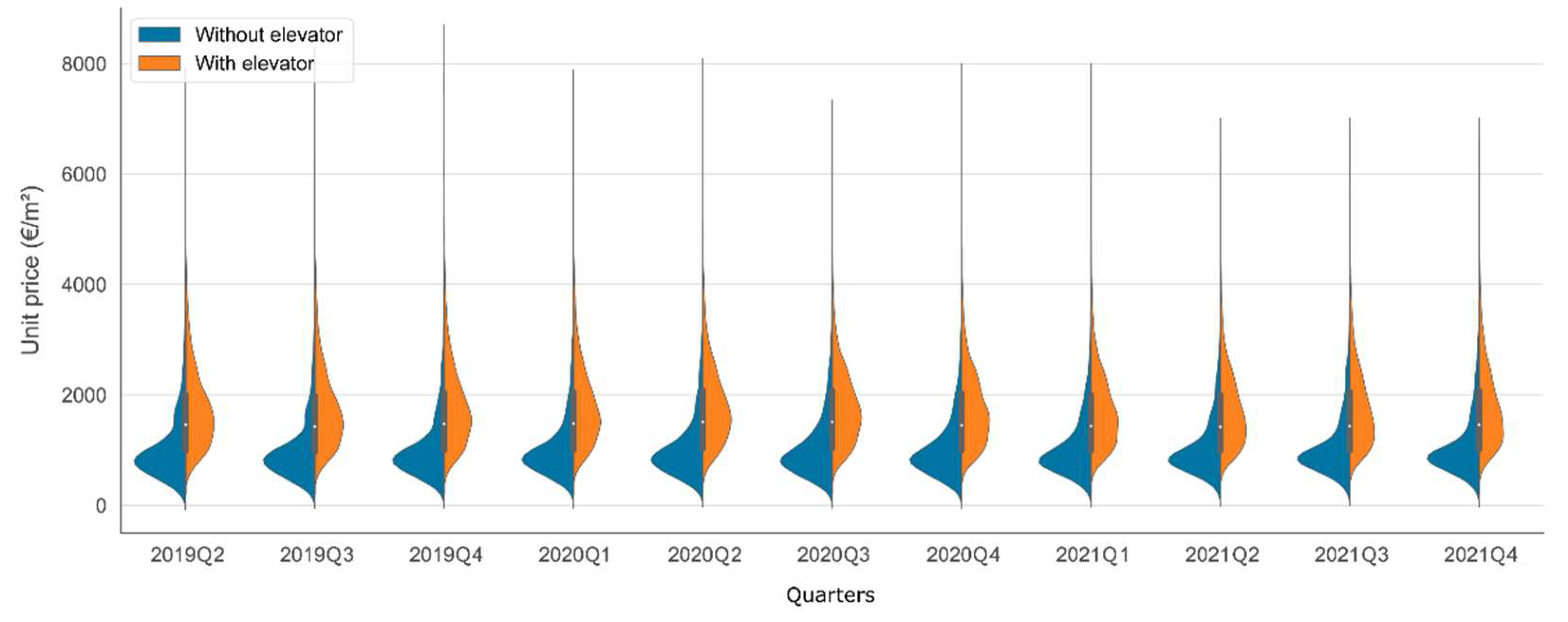
Building characteristics (B)B_elevatorWith (1), Without (0)Availability of elevator
B_parkingWith (1), Without (0)Availability of garage slot
B_storeroomWith (1), Without (0)Availability of storage room
B_poolWith (1), Without (0)Availability of swimming pool
B_gardenWith (1), Without (0)Availability of garden
Location characteristics (C)C_coor_X_kmNumericalProjected coordinates of the spatial location (in kilometers). Coordinate Reference Systems EPSG:25830, with ETRS89 datum and UTM30N projection
C_coor_Y_kmNumerical
Neighborhood characteristics (D)D_age_nbhdNumericalAverage age of the neighborhood (reference year 2021)
D_FARNumericalFloor Area Ratio (total building floor area/gross sector area), 150 m around the building, in m² floor area/m² of the sector
D_dependencyNumericalDependency ratio (sum of the population aged > 64 and <16/population aged 16–64).
D_elderlyNumericalAging ratio (population aged > 64/population aged < 16)
D_foreignersNumericalPercentage of foreign population
D_net_incomeNumericalNet household income for 2019, in thousand euros
D_d_educ1_kmNumericalDistance from the dwelling to level 1 educational centers (infant and primary), in km
D_d_educ2_kmNumericalDistance from the dwelling to level 2 educational centers (secondary and high school), in km
D_d_park_kmNumericalDistance to urban green spaces (parks), in km
D_d_coast_kmNumericalDistance of the dwelling to the coastline, in km
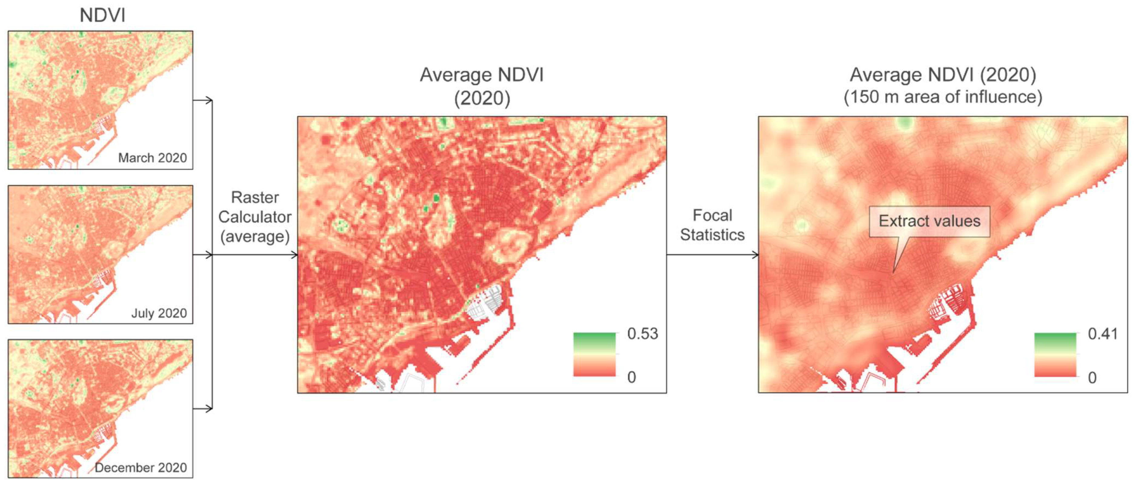
D_NDVI_150mNumericalNormalized Difference Vegetation Index. Average NDVI in a 150 m area of influence
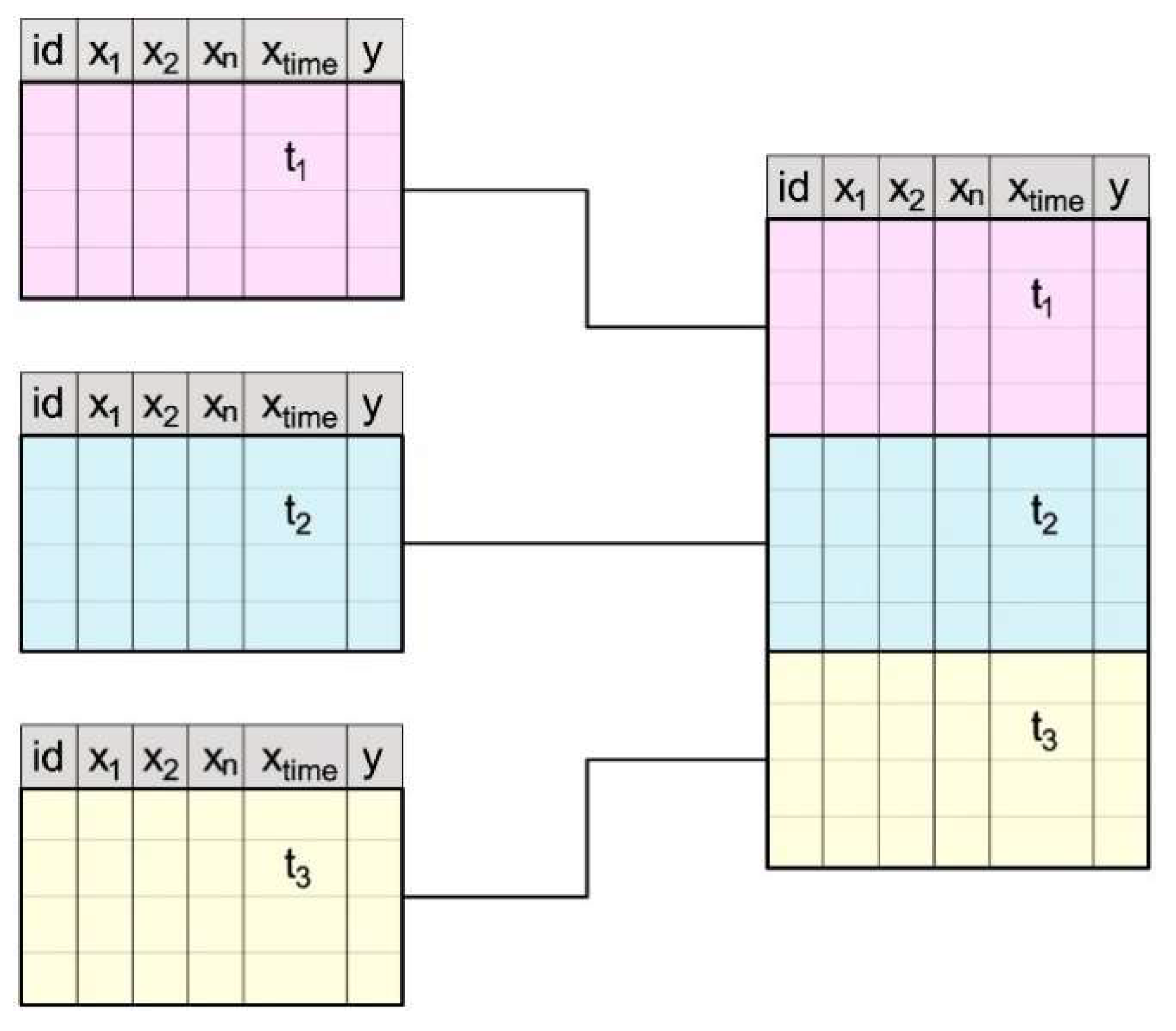
Temporal characteristics (E)E_quarter(Categories)
2019Q2, 2019Q3, 2019Q4, 2020Q1, 2020Q2, 2020Q3, 2020Q4, 2021Q1, 2021Q2, 2021Q3 and 2021Q4
Categorical feature for modeling the time factor in 11 quarters
Dependent featureln_priceNumerical (natural log)The natural log of the asking price offered by the seller (in Euro).
Table 2. Descriptive statistics for the features.
CategoryFeaturesContinuous FeaturesDummy/Categorical Features
MSDMin.Max.CodingFrequency
Dwelling characteristics (A)A_typology (Categories)
Flat
Apartment
Penthouse
Duplex
Studio_flat
Loft

34,073
2758
2397
437
154
124
A_area_m2106.037.620.0340.0
A_bedrooms2.90.81.06.0
A_bathrooms1.60.60.55.0
A_air_cond With (1)
Without (0)
19,555
20,388
A_heating With (1)
Without (0)
12,981
26,962
A_terrace With (1)
Without (0)
4820
35,123
A_new_constr New (1)
No new (0)
870
39,073
Building characteristics (B)B_elevator With (1)
Without (0)
27,600
12,343
B_parking With (1)
Without (0)
13,493
26,450
B_storeroom With (1)
Without (0)
8233
31,710
B_pool With (1)
Without (0)
9259
30,684
B_garden With (1)
Without (0)
4805
35,138
Location characteristics (C)C_coor_X_km720.342.39716.57726.63
C_coor_Y_km4248.351.444239.484252.26
Neighborhood characteristics (D)D_age_nbhd43.7011.6611.50100.40
D_FAR1.780.980.004.95
D_dependency0.530.100.240.92
D_elderly1.871.170.106.45
D_foreigners15.908.391.7048.00
D_net_income30.088.8713.6164.96
D_d_educ1_km0.490.370.012.76
D_d_educ2_km0.560.470.015.94
D_d_park_km0.520.360.002.90
D_d_coast_km1.601.000.035.56
D_NDVI_150m0.080.030.040.26
Temporal characteristics (E)
(*)
E_quarter (Categories)
2019Q2
2019Q3
2019Q4
2020Q1
2020Q2
2020Q3
2020Q4
2021Q1
2021Q2
2021Q3
2021Q4

6264
7329
8203
8372
7232
8482
9516
9498
9462
9725
9941
Dependent feature (*)ln_price11.880.649.4414.27
price178,123129,61112,6001,578,000
Notes: Number of unique properties 39,943. (*) Total number of prices 94,024. M mean, SD standard deviation.
Table 3. Machine learning algorithms used.
IdNameModelLibrary
1lrLinear Regressionsklearn.linear_model.LinearRegression
2rfRandom Forest Regressorsklearn.ensemble.
RandomForestRegressor
3etExtra Trees Regressorsklearn.ensemble.ExtraTreesRegressor
4gbrGradient Boosting Regressorsklearn.ensemble.
GradientBoostingRegressor
5xgbmExtreme Gradient Boostingxgboost.XGBRegressor
6lgbmLight Gradient Boosting Machinelightgbm.LGBMRegressor
Note: the lr algorithm is used as a baseline and for comparative purposes.
Table 4. Results from the initial performance and hyperparameter adjustment by cross-validation (R² score in CV-validation and standard deviation in parentheses).
ModelNameInitial
Hyperparameters
Hyperparameter Optimization
Random (200)Bayesian (100)Best
Linear Regressionlr0.8048
(0.0060)
---
Random Forest Regressorrf0.9036
(0.0049)
0.8869
(0.0037)
[time 37 min 56 s]
0.8855
(0.0038)
[time 30 min 11 s]
Initial hyperparameters
Extra-Trees Regressoret0.9101
(0.0040)
0.8628
(0.0044)
[time 20 min 7 s]
0.8800
(0.0039)
[time 38 min 42 s]
Initial hyperparameters
Gradient Boosting Regressorgbr0.8581
(0.0054)
0.9101
(0.0035)
[time 53 min 28 s]
0.9125
(0.0034)
[time 39 min 32 s]
Bayesian
Extreme Gradient Boostingxgbm0.8921
(0.0034)
0.9094
(0.0041)
[time 1 h 3 min 36 s]
0.9077
(0.0039)
[time 45 min 10 s]
Bayesian
Light Gradient Boosting Machinelgbm0.8864
(0.0042)
0.9065
(0.0043)
[time 28 min 42 s]
0.9076
(0.0044)
[time 16 min 17 s]
Bayesian
Table 5. Performance results of the trained algorithms (R² score).
ModelNameCV-Validation in Training Set (SD)R² Score
Training SetTest SetOverfitting (%)
Linear Regressionlr0.8048 (0.0060)0.80560.8052-
Random Forest Regressorrf0.9036 (0.0049)0.99700.9135+9.1
Extra-Trees Regressoret0.9101 (0.0040)0.99970.9178+8.9
Gradient Boosting Regressorgbr0.9125 (0.0034)0.99520.9192+8.3
Extreme Gradient Boostingxgbm0.9094 (0.0041)0.99000.9178+7.9
Light Gradient Boosting Machinelgbm0.9076 (0.0044)0.99020.9140+8.3
Table 6. Error and goodness-of-fit measures for the algorithms on different datasets (various metrics).
Model NameTest Dataset (30%)Complete Dataset (Training + Test, 100%)
MAEMSERMSEMAEMSERMSE
lr0.21660.07970.28230.80520.21630.07990.28260.8055
rf0.12520.03540.18820.91350.01780.00120.03480.9971
et0.12190.03360.18340.91780.00190.00020.01420.9995
gbr0.12640.03310.18180.91920.03640.00290.05360.9930
xgbm0.12980.03360.18340.91780.05070.00510.07140.9876
lgbm0.13220.03520.18760.91400.05250.00570.07530.9862
Publisher’s Note: MDPI stays neutral with regard to jurisdictional claims in published maps and institutional affiliations.

