Simple Optimal Sampling Algorithm to Strengthen Digital Soil Mapping Using the Spatial Distribution of Machine Learning Predictive Uncertainty: A Case Study for Field Capacity Prediction

Abstract

Machine learning models are now capable of delivering coveted digital soil mapping (DSM) benefits (e.g., field capacity (FC) prediction); therefore, determining the optimal sample sites and sample size is essential to maximize the training efficacy. We solve this with a novel optimal sampling algorithm that allows the authentic augmentation of insufficient soil features using machine learning predictive uncertainty. Nine hundred and fifty-three forest soil samples and geographically referenced forest information were used to develop predictive models, and FCs in South Korea were estimated with six predictor set hierarchies. Random forest and gradient boosting models were used for estimation since tree-based models had better predictive performance than other machine learning algorithms. There was a significant relationship between model predictive uncertainties and training data distribution, where higher uncertainties were distributed in the data scarcity area. Further, we confirmed that the predictive uncertainties decreased when additional sample sites were added to the training data. Environmental covariate information of each grid cell in South Korea was then used to select the sampling sites. Optimal sites were coordinated at the cell having the highest predictive uncertainty, and the sample size was determined using the predictable rate. This intuitive method can be generalized to improve global DSM.

1. Introduction

Field capacity (FC) is one of the main factors representing the hydrologic characteristics of the soil. It refers to the water content when its gravity-induced vertical movement speed through the soil is reduced [1]. Because the term is frequently used to describe the actual quantity of water in the soil that plants can use, it is actively leveraged as an input variable in hydrologic models [1,2]. Therefore, a proper understanding of the spatial FC distribution is essential for sustainable water management, especially in forested areas.

The digital soil mapping (DSM) technique is widely used to predict the soil properties of interest (e.g., FC and hydraulic conductivity) using geographically referenced information or remote sensing (big) data [3,4]. DSM is a geospatial technique that can handle numerous variables that describe soil properties as data accumulate over time. It can predict the soil properties of large areas. To map the distribution of soil properties, information on soil properties is analyzed from the soil investigation first. Then, environmental covariate information corresponding to the points where soil samples were collected is extracted through the available geographically referenced data. After this, a predictive model for estimating soil properties is developed through the relationship between soil properties and extracted environmental covariates. When the raster-based information of environmental covariates is used as input data for the model, then it is possible to predict the soil properties in cell units and map the distribution of soil properties. In the past, it was not easy to use DSM because it took a lot of time to process a large amount of data at once. Further, it used a parallel computing technique involving multiple computers. However, computing speeds have improved drastically, as have the various dedicated processors. Additionally, several working DSM machine learning algorithms have been developed. With the accumulation of spatial big data, these algorithms have become extremely useful for understanding the growing quantitative relationships between field values and laboratory measurements. Therefore, researchers are creating prediction models with very high accuracy.

Data-driven machine learning models are strongly influenced by the available data and the quality of the training datasets used to train them [5,6]. For example, even if the number of input data is large, but the data quality is low, the prediction performance will be poor, and the predictive uncertainty will be significant. Even when the data quality is high, the prediction power will suffer if the amount is insufficient because the correlation between variables cannot be fully understood after training. Therefore, a sufficient amount of high-quality data must be collected to successfully develop an excellent predictive model. Moreover, it is essential to have an appropriate investigation plan because collecting data, especially in forests, is time-consuming.

Many sampling algorithms for effective investigation plans for DSM have been proposed until now [7,8]. When we do not have any collected dataset, some methods can choose sampling sites such that their distribution can cover all target sites [8,9]. Further, sampling sites can be randomly selected according to the purpose of the researchers [10]. However, after collecting some data from the field, we can choose other methods for sampling design, since we can understand the characteristics of the variables of interest more deeply from the collected data. Nevertheless, we cannot rely on random sampling for precision metrics. Moreover, we can never know all the features encountered at a new study site. Hence, after sample data collection and during a study, one must identify the missing features and compensate for them to avoid incorrect machine learning inferences caused by faulty extrapolations. Notably, there are usually many variables to consider, owing to the multivariate characteristics of DSM and the complex nature of the Earth’s geology [10]. Therefore, one must pause the study to sample additional sites, leverage additional (perhaps poorly fitting) datasets, or derive environmental covariates (given linear relationships and discrete variables). However, with soil studies, continuous variables are the most common types encountered, and most have nonlinear relationships with the target variable, rendering discretization difficult, even with augmented data.

The National Institute of Forest Science has collected many forest soil samples to estimate FC in forested areas until now and wants to select additional sampling sites to improve the existing DSM. However, few studies have been conducted on determining the optimal sample size or coordinating the sampling locations while considering the characteristics of all variables in this situation. Moreover, not many sampling algorithms using machine learning have been reported.

This study aims to (1) develop a hierarchical predictive model to predict FC based on the data collected until now in Korean forests on a national scale and (2) select optimal sampling sites to strengthen the developed DSM model effectively. To this end, hierarchical predictive models have been developed based on the data collected until now. In addition, a simple optimal sampling algorithm is proposed through the relationship between the predictive uncertainty of the machine learning model and the distribution of the training dataset. Finally, this method is applied to the entire nation of South Korea, and the optimal sample size and coordinates of sampling sites are suggested.

2. Materials and Methods

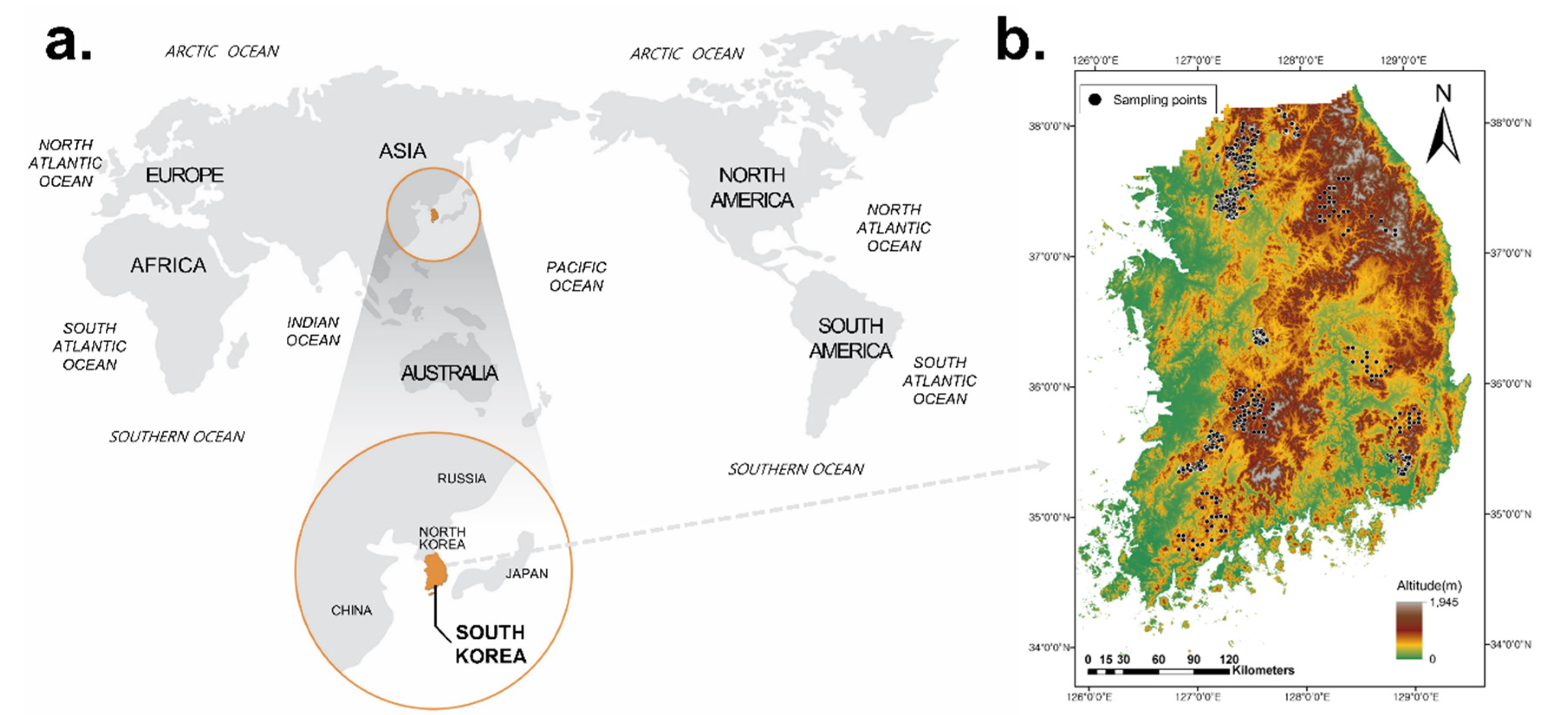
2.1. Study Sites

South Korea is located in the range of 33–43° latitude and 124–132° longitude in Southeast Asia (Figure 1), bordered to the north by North Korea and surrounded by water on the other three sides. Thus, it is influenced by the characteristics of the Asian continent and oceanic air masses. Located in a temperate climate zone, it has four seasons, with annual average precipitation of 1343 mm and average temperatures of 23–25 Celsius. Extensive forests have been cultivated since the 1970s, and most of the nation is now fully covered. The Baekdudaegan watershed occupies most of the north–south length of the country, providing vast spatial variability throughout. Figure 1 presents South Korea’s general global location and a map of current soil sample sites.

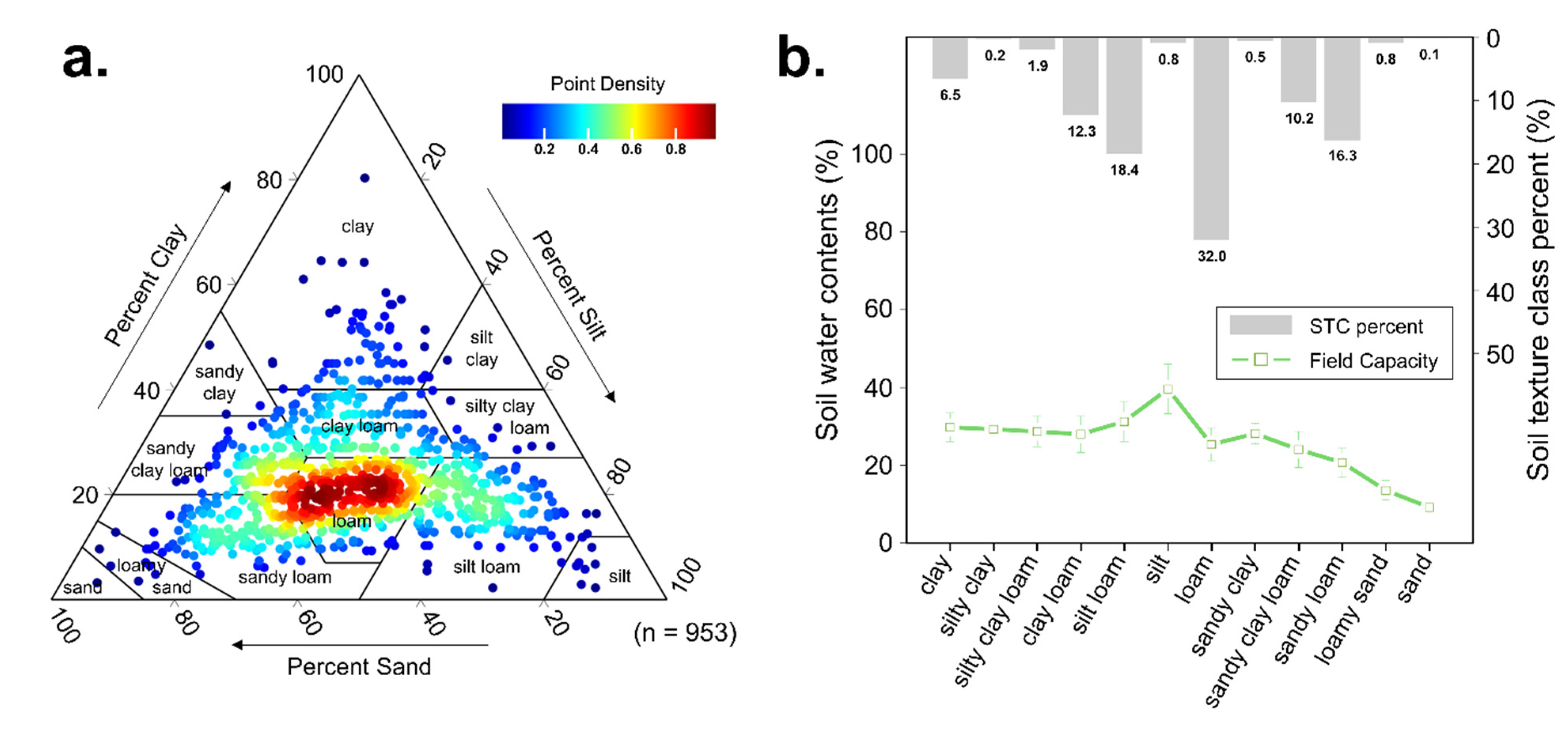
2.2. Collected Soil Samples and Their Properties

This study was conducted using the data from forest topsoil samples collected over time from 953 sites by workers at the National Institute of Forest Science (Figure 1). Samples were collected at 10 cm levels (mineral A horizon), and six soil properties, including FC, were applied in this study, based on the study of Yang et al. [11], in which the detailed analysis process was first suggested. All 953 soil samples were collected randomly since there was no previous information about the forest soils and their relationship with other environmental variables. In addition to this, soil sampling was conducted seven days after the rain to eliminate the climatological effects. Moreover, all soil properties were analyzed with the same method, which means that there was consistency in the soil property data. Descriptive statistics for the six forest soil properties are shown in

Table 1. Descriptive statistics for forest soil properties used in this study.

Soil Properties	Abb.	Unit	Min	Mean	Max	Std.	Skew.	Kurt.
Field capacity	$\mathrm{FC}$	%	9.2	26.3	50.5	5.8	0.5	0.8
Sand fraction	Sand	%	3.3	39.5	91.0	16.3	0.2	−0.4
Silt fraction	Silt	%	1.5	37.6	87.3	15.7	0.6	0.0
Clay fraction	Clay	%	2.2	22.8	80.3	10.3	1.3	2.4
Bulk density	${\mathsf{\rho }}_b$	g cm−3	0.4	1.0	1.5	0.2	0.1	−0.3
Organic matter	OM	%	2.1	11.2	38.1	4.5	1.1	2.4

Abb, abbreviation; FC, field capacity; OM, organic matter; Std, standard deviation; Skew, skewness; Kurt, kurtosis; ${\mathsf{\rho }}_b$, bulk density.

.

Soil size distribution (e.g., sand, silt, and clay fraction) was analyzed using the hydrometer method. The soil texture class (STC) was classified using the US Department of Agriculture (USDA) texture classes, whose textural classes and FC distributions are shown in Figure 2. Considering that the sample collection was randomly conducted at first, loam is currently the most distributed soil texture class in forested areas of South Korea.

2.3. Forest Environmental Covariates

South Korea has two essential big data forest type and characteristic site datasets: Forest Site and Soil Map (FSSM) and Forest Type Map (FTM). In this study, the Geologic Map (GM; 1:50,000), FSSM (1:25,000), FTM (1:25,000), and Digital Elevation Map (DEM; 10 m resolution) datasets were used to extract 14 forest environmental covariates; the detailed information about each variable is listed in Table S1. Some environmental covariates derived from DEM (e.g., topographic position index (TPI), aspect, profile curvature, plan curvature, topographic wetness index, and upper catchment area) were calculated using a geospatial information system analyst tool.

2.4. Machine Learning Algorithms

Many studies on soil hydraulic properties have used machine learning algorithms for their high predictive accuracy and dimensionality [12,13]. This study tested and compared four widely used models: gradient boosting, random forest, k-nearest neighbors, and multilayer perceptron. For the training of the four models, the optimal hyperparameter determining the structure of the model was found using the grid searching method. Grid searching was performed 20,000 times each to find the optimal hyperparameter sets in this study. We used Python v.3.7.4 and SciKit-Learn v.1.1.2. to run these machine learning models.

2.4.1. Gradient Boosting (GB)

GB is an ensemble method that enhances the prediction accuracy by combining the results of multiple individual base classifiers [12,14]. Although other machine learning models (e.g., decision trees and RF) focus on improving performance, the gradient of the GB retains the weak residual errors learned until the present cycle [15]. This approach reduces noisy data using decision trees and continuous runs. Eventually, GB lowers the mean-squared error (MSE) by repeatedly training to correct those caused by earlier iterations [16]. This study’s three hyperparameters were tuned for GB optimization: n_estimators, learning_rate, and max_depth.

2.4.2. Random Forest (RF)

RF was developed by Breiman [17] as a decision tree algorithm that combines a bagging method with random variable selection [18]. Multiple training data are created from a single dataset, and several more are produced by combining the decision trees, which increases the predictability via reintegration [15]. Because it is indifferent to the range of input values, RF is resistant to overfitting [19]. Three hyperparameters were tuned for RF optimization: n_estimators, max_depth, and max_features.

2.4.3. K-Nearest Neighbors (KNN)

The KNN is a basic nonparametric technique that classifies unknown instances using known instances as the baseline [19]. The maximum summed densities are calculated to identify and classify the closest k neighbors. Because KNN can estimate complicated and/or nonlinear problems, it has been used to analyze large datasets simultaneously [20] for soil mapping [21]. Three hyperparameters were tuned for KNN optimization: leaf_size, p, and n_neighbors.

2.4.4. Multilayer Perceptron (MLP)

The MLP neural network is one of the most common algorithms owing to its minimal training needs and simple utility [19,22]. MLP creates many basic units (i.e., neurons) capable of making simple decisions based on learning from training samples [12]. A neuron uses interconnected layers to make final predictions by feeding those decisions to other neurons, depending on the activation function. Generally, three layer types comprise an MLP network: input, hidden, and output. In this study, the optimal number of neurons in the hidden layer was determined by trial and error and was the only hyperparameter tuned.

2.5. Variable Importance

2.5.1. Variance Inflation Factor (VIF)

The variable importance measurement method produces inaccurate results when there is an interrelationship between variables [17]. VIF is the most commonly used method for quantifying variable correlation [23]. The VIF value for a single variable is derived as follows:

$${\mathrm{VIF}}_{X_1}=\frac{1}{1-R_{X_1}^2}$$

(1)

where R² is the coefficient of determination of the multiple linear regression equation, in which variable $X_1$ is the response variable, and the others ($X_2, X_3, \dots ,X_N$) are explanatory variables. Generally, when the VIF is greater than five, a correlation between variables exists, and the corresponding variable must be eliminated before the variable importance can be accurately calculated [24].

2.5.2. Feature Importance

Feature importance is based on the mean decrease in impurity [17]. It is related to the decision tree building process, in which a decision tree splits to obtain the most significant modes of impurity reduction. The more the impurity can be reduced, the higher the variable importance. Using this principle, feature importance is one of the most commonly used methods for estimating variable importance because it is provided by most RF tools and is easily applicable [17,25]. Feature importance can only be derived using the RF model. After an optimal hyperparameter set is selected, the RF model is developed, and the feature importance is averaged from 100 bagging cycles as slightly different results are provided in each round. We used SciKit-Learn v.1.1.2 for this purpose.

2.5.3. Permutation Importance

Permutation importance is another method of estimating variable importance, and it is based on the mean decrease in accuracy. The general method permutes one test set variable after model development, while the other variables are kept constant. The permutation decrease is then reflected in the model accuracy (e.g., via the coefficient of determination; [26]). With a single dependent variable, model accuracy significantly decreases when permuted [17]. In this study, 50 permutations were conducted per variable. Unlike feature importance, permutation importance applies to all model types. Additionally, the results of premutation importance estimation are directly affected by splitting the data into training and testing sets. Thus, data splitting was randomly conducted 100 times, and permutation importance was the averaged value of 100 results.

2.6. Predictor Set Hierarchy

In most cases, the proper predictor set is selected to simplify the model as much as possible while maintaining the prediction performance [27]. A stepwise statistical method is used, and several predictor sets may be constructed for performance comparisons. In this study, in addition to this, there is one additional purpose of comparing the performance of different predictor set hierarchies.

Currently, in South Korea, continuous forest surveys are being conducted, and geographically referenced information (e.g., FSSM, GM, and FTM) and in situ forest soil measurements are continuously updated. It means that data coverage varies by location. For the most accurate FC prediction, it is crucial to predict it using a hierarchy model with the maximum accuracy for each location. Considering the above criteria, six predictor set hierarchies were constructed in this study.

If the variables have correlations, a multicollinearity issue may occur, and the accuracy of model prediction may decrease. To prevent this, the VIF analysis described in Section 2.5.1 was performed, and each predictor set was configured so that no correlated variables would be included. For example, soil texture class and sand have VIF values of 5 or more, so one of the two variables should be removed from E14-S2 and E14-S4, where these two factors overlapped. In order to minimize the decrease in the predictive models’ performance, we removed the variable that did not explain FC relatively well. In this study, feature importance was used to determine the more important variable for prediction. In this case, sand had higher feature importance and the soil texture class was eliminated.

2.7. Performance Evaluation

Model performance was evaluated using our developed model and a hold-out test set that was not used for training. In particular, 80% of the total data was used for training, and 20% was used for testing. Five-fold cross-validation was used for performance evaluation. To assess the model performance in each evaluation process, the Nash–Sutcliffe model efficiency (NSE) coefficient, which is very effective in assessing predictive performance, and the root mean-squared error (RMSE) were used. These evaluation methods are defined as follows:

$$\mathrm{NSE}=1-\frac{{{\displaystyle \sum }}_{i=1}^N{\left[\widehat{F{C}_i}-F{C}_i\right]}^2}{{{\displaystyle \sum }}_{i=1}^N{\left[\overline{F{C}_i}-F{C}_i\right]}^2}$$

(2)

$$\mathrm{RMSE}=\sqrt{\frac{1}{N}{{\displaystyle \sum }}_{i=1}^N{\left[\widehat{F{C}_i}-F{C}_i\right]}^2}$$

(3)

where N is the number of soil samples, $\widehat{FC}$ is the modeled FC, and $\overline{FC}$ is the average value of the measured FCs.

2.8. Statistical Analysis

Several statistical analytical methods were used in this study. Performance evaluation and descriptive statistics (e.g., average value, standard deviation, skewness, and kurtosis) were performed with Numpy v.1.17.3 with Python v.3.7.4 by Python Software Foundation in Delaware, United States.

3. Results and Discussion

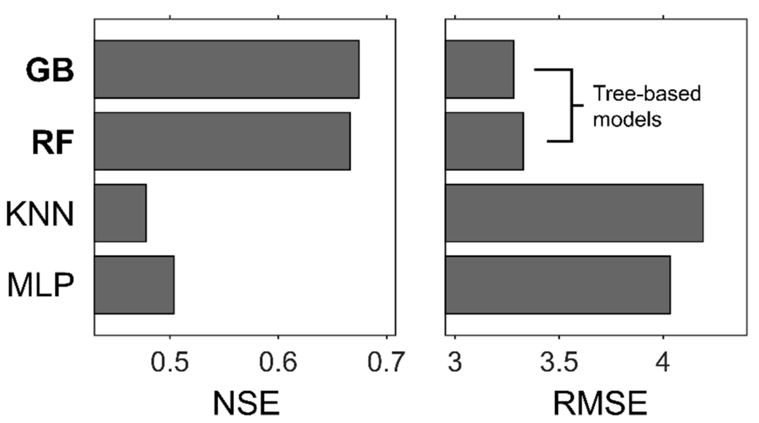
3.1. Optimal Machine Learning Algorithm for FC Prediction

The model performance of GB, RF, KNN, and MLP was assessed to find the optimal machine learning algorithm for FC prediction. The E14-S4 predictor set hierarchy was used to develop the performance comparison model (see

Table 2. Six predictor set hierarchies, the input variables of each hierarchy, and their data sources.

Hierarchy ID	Input Variables	Data Sources
E4-S0	STC, TSD, SC, Hardness	FSSM
E12-S0	STC, TSD, SC, Hardness, Elevation, Slope, Aspect, CA, TWI, TPI, ProC, PlanC	FSSM, DEM
E14-S0	STC, TSD, SC, Hardness, Elevation, Slope, Aspect, CA, TWI, TPI, ProC, PlanC, Bedrock, FT	FSSM, DEM, GM, FTM
E0-S4	$\mathrm{Sand},\mathrm{Clay},\mathrm{OM},{\mathsf{\rho }}_b$	In situ measurement
E14-S2	TSD, SC, Hardness, Elevation, Slope, Aspect, CA, TWI, TPI, ProC, PlanC, Bedrock, FT, Sand, Clay	FSSM, DEM, GM, FTM, in situ measurement
E14-S4	$\mathrm{TSD},\mathrm{SC},\mathrm{Hardness},\mathrm{Elevation},\mathrm{Slope},\mathrm{Aspect},\mathrm{CA},\mathrm{TWI},\mathrm{TPI},\mathrm{ProC},\mathrm{PlanC},\mathrm{Bedrock},\mathrm{FT},\mathrm{Sand},\mathrm{Clay},\mathrm{OM},{\mathsf{\rho }}_b$	FSSM, DEM, GM, FTM, in situ measurement

DEM, Digital Elevation Map dataset; FSSM, Forest Site and Soil Map dataset; FTM, Forest Type Map dataset; GM, Geologic Map dataset; STC, soil texture class; TSD, total soil depth; SC, stone content; CA, catchment area; TWI, topographic wetness index; TPI, topographic position index; ProC, profile curvature; PlanC, plan curvature; FT, forest type; OM, organic matter; ${\mathsf{\rho }}_b$, bulk density.

), and NSE and RMSE with five-fold cross-validation were applied.

Figure 3 shows that GB and RF performed better than KNN and MLP. GB and RF showed a higher NSE, which reflects good accuracy (the closer to one, the higher the predictive power). Moreover, GB and RF showed a smaller RMSE, which reflects low errors between the predicted and true values. Both the GB and RF models are based on decision trees, with splitting paths but no converging ones. Decision rules are used for splitting; hence, two leaves are created each time. The tree grows more significantly as the amount of information from the input data and its complexity increase [28]. Owing to these characteristics, the GB and RF models can be trained without being affected by the scale of the input data and variables (continuous or discrete).

For example, there are three categories of bedrock used in this study. Because all input data of a machine learning model must consist of numeric variables, igneous rock was converted to 1, sedimentary rock to 2, and metamorphic rock to 3. However, this does not mean that the scale of characteristics of metamorphic rock is three times that of igneous rock. In this case, the decision tree can effectively categorize these three characteristics.

KNN, on the other hand, measures the distances between two data values to evaluate similarities [29]. The Euclidean distance is $\sqrt{{\left(x_1-x_2\right)}^2+{\left(y_1-y_2\right)}^2}$, in which $(x_1,y_1)$ and $(x_2,y_2$) are coordinates. In other words, effective analysis becomes difficult when discrete data are converted into numeric variables. As MLP is a fully connected feed-forward artificial neural network [12], the activation functions and node weights are included in each calculation process; hence, the results can be negatively affected by the scale of the categorical data when converted into continuous values [30]. Therefore, although GB and RF can effectively process these datasets, KNN and MLP cannot. Several methods have been proposed to overcome this problem, such as one-hot encoding [31]. However, these methods will not be discussed further here because they are beyond the aim and scope of this paper.

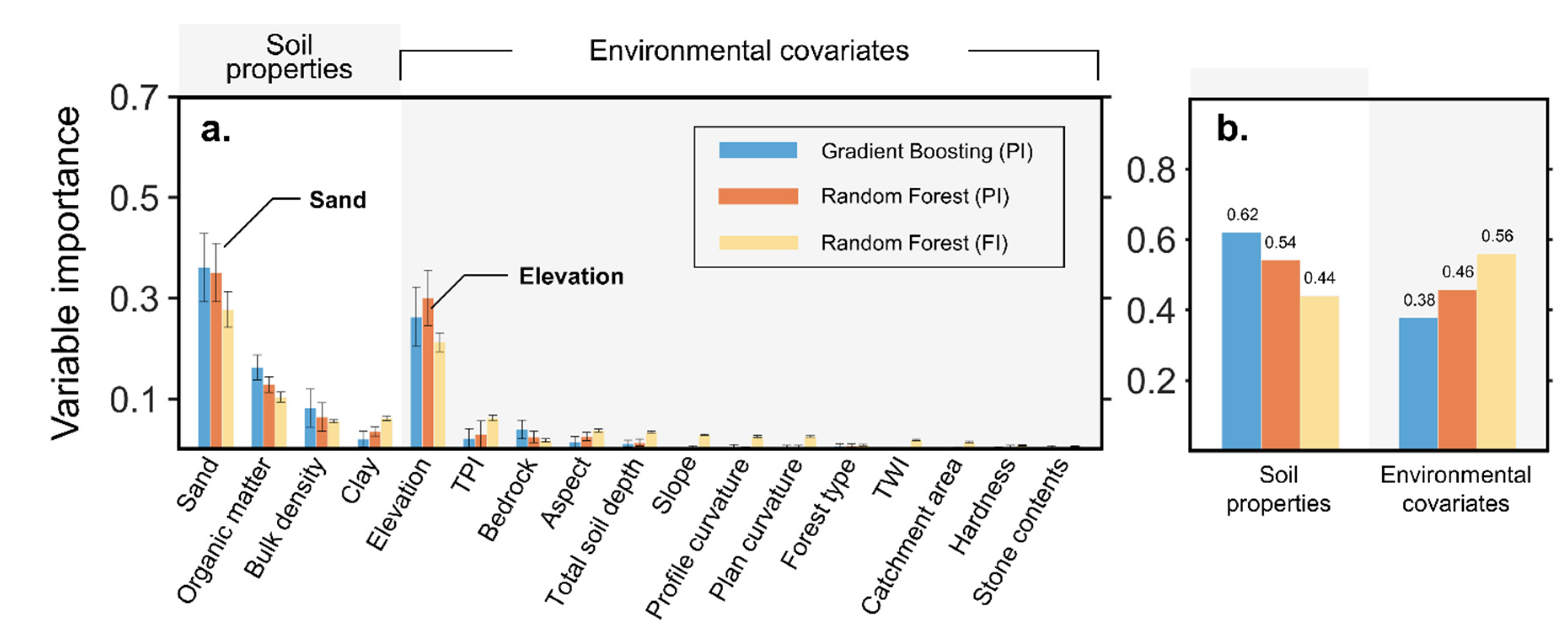
3.2. Relationship between Predictors and FC

The GB and RF models were used to analyze the predictor importance for estimating FC, noting that tree-based models are the most suitable. Three methods were used to verify the importance of variables: permutation importance of GB and RF and feature importance of RF. There were slight differences among these methods, but the variables significantly influencing the prediction of FC showed similar trends (Figure 4). Among the soil properties, sand and organic matter were important in predicting FC, and elevation and TPI were important among the environmental covariates. With GB, the influence of soil properties was more important than environmental covariates. However, in the RF model, the influence of environmental covariates was quite similar to that of soil properties. Therefore, it was found that using the RF model was more advantageous for the E4-S0, E12-S0, and E14-S0 predictor set hierarchies, which mainly use environmental covariates as predictors. Alternatively, the GB model was more advantageous for E0-S4, E14-S2, and E14-S4, which mainly use soil properties as predictors.

A 2D heatmap was drawn, as shown in Figure S1, to visualize the effect of each variable on FC and their correlations. To verify the effect of environmental covariates on FC, a 2D heatmap matrix was prepared with the top four variables selected through importance analysis (Figure S1). The E14-S0 predictor set hierarchy-based RF model was trained to verify the effect of environmental covariates on FC. To consider only the effect of the two variables of interest, one soil type used in the training set was selected. The FC was predicted by modifying only the two variables, whereas the others remained fixed. The process of predicting FC by selecting soil was performed 500 times. After calculating the average of the results, it was standardized to a value between zero and one so that the trend could be checked more directly. The equation for standardization is as follows: $F{C}_i^{\prime }=\left(F{C}_i-F{C}_{min}\right)/\left(F{C}_{max}-F{C}_{min}\right)$. The effect of soil properties on FC was examined using the E0-S4 predictor set hierarchy-based GB model. It was found that the FC value decreased as the elevation decreased, the TPI approached zero, and the aspect was closer to the south. Regarding bedrock, the FC of forest soil with igneous rock as bedrock was higher than the others. The result showed that as the sand decreased and the bulk density, organic matter, and clay increased, the FC increased, and the correlation between each variable was easily confirmed (Figure S2).

Sand, OM, elevation, and TPI were the most important variables to predict FC. The interrelationship between soil properties and topographical features was analyzed by Yang et al. [11] using the same soil samples in South Korea. In this paper, however, we briefly discuss the relationship between FC and the important variables. FC is highly correlated with capillary force, affected by the soil texture, which determines the micropores [32]. Silt and clay fractions in soils have a great influence on the capillary force, and as the sand fractions increase, the content of silt and clay decreases, meaning that FC tends to decrease [11]. Organic matter particles attract water and can cause water to adhere to the soil surface [33]. This is the main reason that the OM has higher variable importance. Hudson [34] also stated that OM has a significant impact on the available water capacity. In Figure S1, elevation and TPI show a positive relationship with FC. Elevation was highly correlated with OM and sand in South Korea. One of the reasons is that the nationally protected area that is strictly limited is mostly distributed in Baekdudaegan, which is a higher-altitude area [11]. TPI represents the slope position, and it has a negative value at the ridge and a positive value at the valley [35]. Since most of the ridges—showing higher TPI values—are distributed in Baekdudaegan, TPI is an important variable and has a positive relationship with FC.

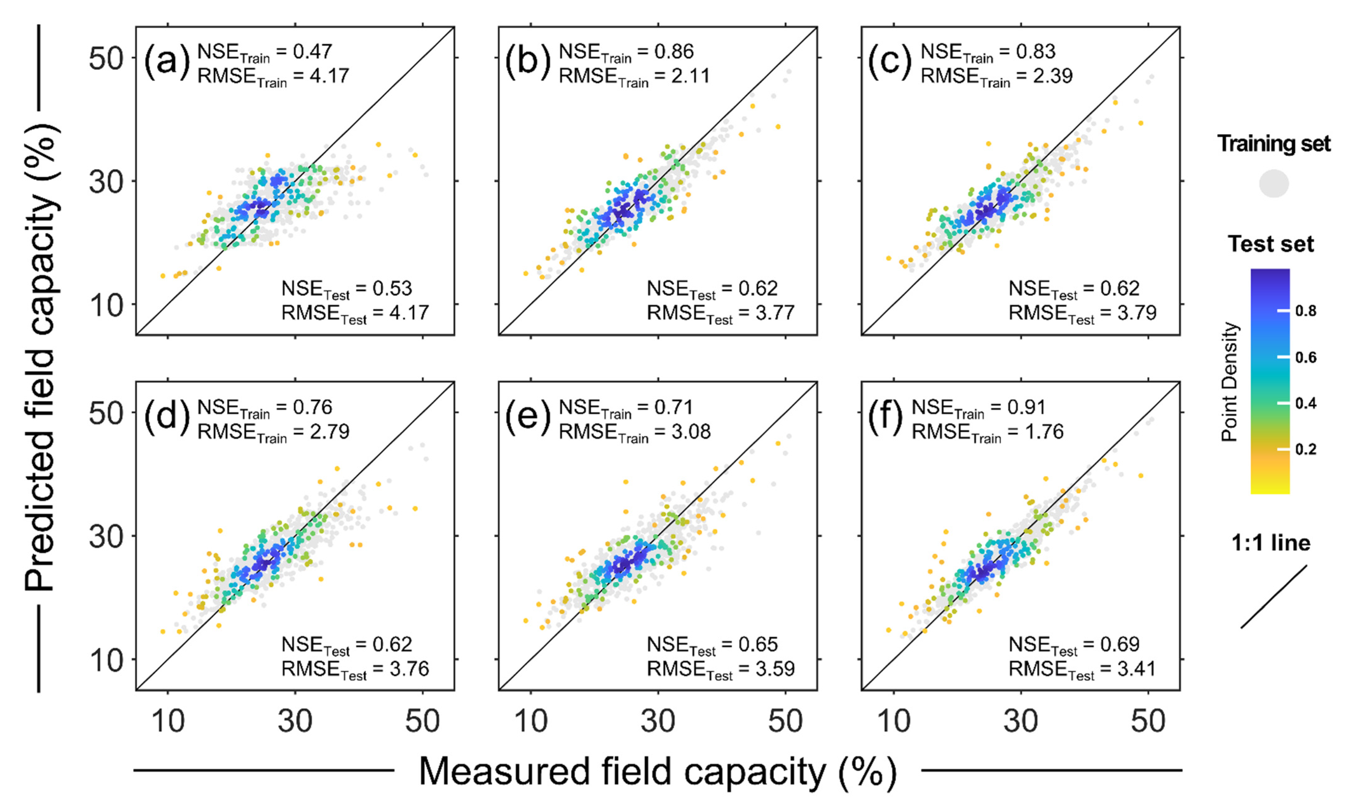
3.3. Model Performance Evaluation by Different Predictor Set Hierarchies

FC prediction using the six predictor set hierarchies was performed to cover the spatially differentiated data with optimal accuracy (Table 2). The machine learning models were paired with their optimal predictor set hierarchies as follows: E4-S0 (RF), E12-S0 (RF), E14-S0 (RF), E0-S4 (GB), E14-S2 (GB), and E14-S4 (GB).

To compare the prediction performance of each predictor set hierarchy, the measured and predicted FCs were compared (Figure 5). A scatterplot of five-fold cross-validation was built by arbitrarily selecting one of the five validations. The E4-S0 predictor set hierarchy showed the lowest predictive performance, whereas there was little difference among E12-S0, E14-S0, and E0-S4. The predictive accuracy increased as the number of soil property types increased, and the E14-S4 model showed the highest performance.

Notably, the E14-S0 and the E0-S4-based models’ performance was almost identical. The E14-S0 model can represent the DSM, and the E0-S4 model can represent the pedo-transfer function (PTF). The PTF model predicts another soil property of interest based on the soil’s physical and chemical properties [36]. Therefore, the predictive power of PTF, which directly predicts soil characteristics, is generally higher than that of DSM, which predicts soil characteristics based on indirect environmental variables [37]. Although PTF has the advantage of relatively high predictive power, its disadvantage is that it is difficult to predict a large area because it can predict only the soil characteristics of the site from which the soil was directly investigated [38]. On the contrary, DSM has lower predictive power than PTF, while it can predict a broader range of soil properties [11]. However, the data collected in this study indicate that the explanatory power of environmental covariates is already very similar to the explanatory power of soil properties.

In other words, the number of geographically referenced datasets collected so far in Korea is as abundant, as it can follow the explanatory power of in situ measurement. Furthermore, it can be seen that the characteristics of environmental covariates and soil properties do not overlap because the performance of E14-S2 (Figure 5e,f), which combines these two datasets, further increased.

The FC of South Korea was predicted using all six hierarchical sets (Figure 6), and the averaged FC across the nation was found to be 24.70%. Notably, higher FCs are found at higher altitudes, distributed mainly along the Baekdudaegan watershed crest line. Additionally, the FCs in the northeast and southwest regions, with relatively higher altitudes, were higher than those in the northwest and southeast regions.

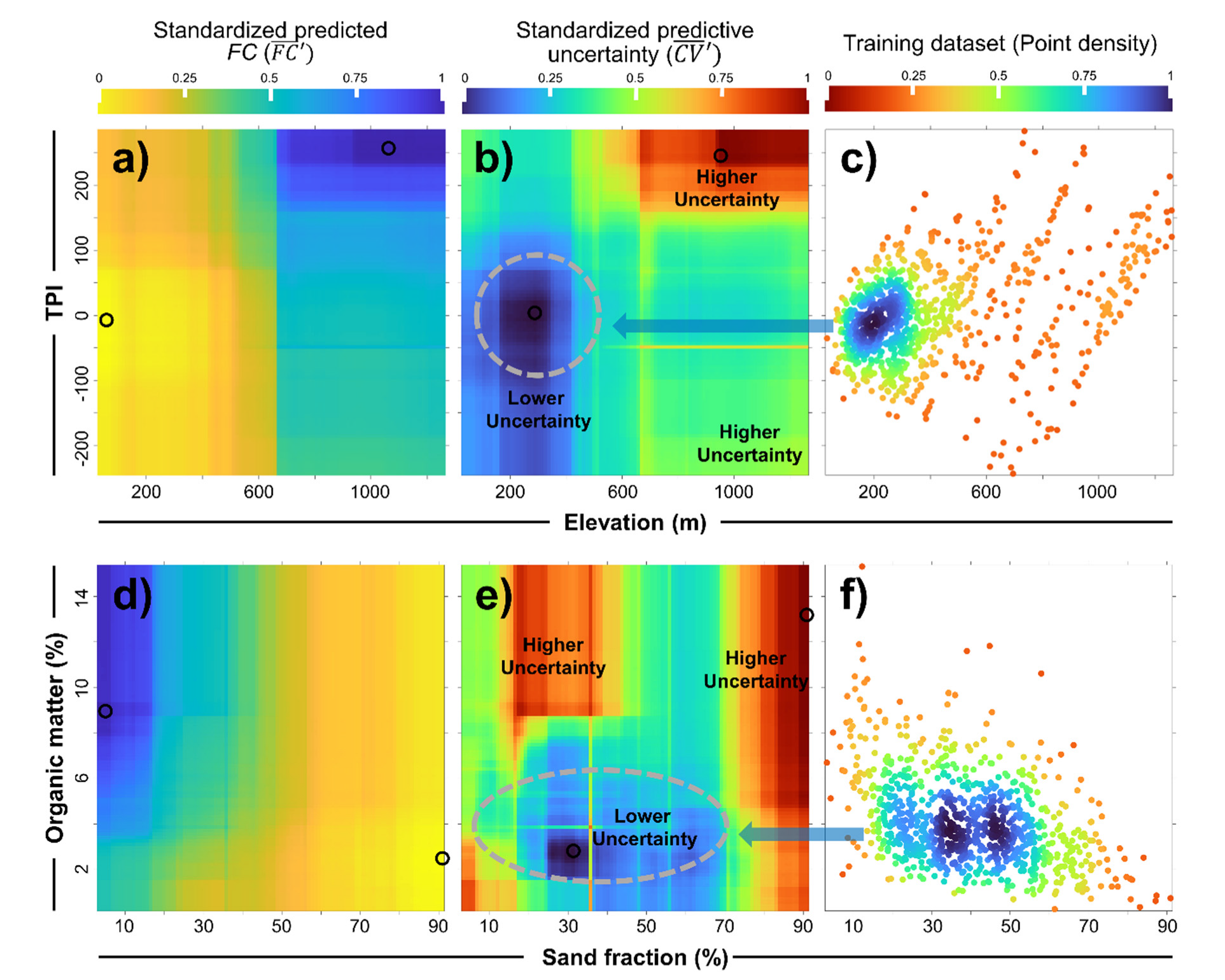
3.4. Relationship between Predictive Uncertainty and Distribution of Training Datasets

The E14-S0 and E0-S4 predictor set hierarchy-based RF models were used to estimate the predictive uncertainty of the models. Here, 2D heatmaps were drawn with the two most important variables among environmental covariates and soil properties. We also compared the predicted FC and the distribution of training data alongside predictive uncertainty (Figure 7). One soil sample from the training data was selected to obtain the predicted FC. FC was predicted by modifying only the two variables of interest, while the others remained fixed. The soil samples were selected 500 times, and the prediction was repeated to understand the general trend. Then, the result values were averaged, which was standardized to zero and one to check the relative differences (Figure 7a,d). Predictive uncertainty was derived using the bagging algorithm of the RF model. After selecting the optimal hyperparameter of the model via grid searching, the FC was predicted while continuously changing the randomness of the bootstrapping method. In the “RandomForestRegressor” library of SciKit-Learn, the parameter “random_state” controls randomness. Note that the soil samples used to obtain the predictive uncertainty were the same as those used to obtain the standardized predicted FC. The coefficient of variation (CV; standard deviation/average) values from 500 results were extracted and standardized to zero and one to check the relative difference (Figure 7b,e).

A strong correlation between predictive uncertainty and the distribution of the training dataset was observed, whereas the predicted FC and predictive uncertainty were not found to be significantly related (Figure 7). The part with relatively low predictive uncertainty (blue area in Figure 7b,e) coincides with an extensive training set distribution. Moreover, the part with relatively high predictive uncertainty (red area in Figure 7b,e) corresponds to the part where the training set was barely distributed.

We added training data and simulated how the predictive uncertainties changed to verify the relationship between training data scarcity and predictive uncertainty (Figure 8). We used the E14-S0 predictor set hierarchy-based RF model. After selecting a soil sample, only the elevation and TPI of the soil sample were changed to create 2D imaginary soils—a simple version of the target site. The higher predictive uncertainties were distributed in the upper-left, upper-right, and lower-right corners, where the training data were rarely undistributed. The highest uncertainty was observed in the upper left and was added to the training dataset, assuming that this soil was collected. Here, the FC value of the added data was calculated based on the predicted value of the E14-S0 predictor set hierarchy-based model. Note that a specific error was added to the predicted value because the FC value of the actual soil was different from the model’s predicted value. This error follows the distribution of the difference between the predicted and measured values of the training data using the E14-S0 predictor set hierarchy-based model (see Appendix A). As a result of the simulation, by adding a new soil sample to the training data and observing the changes in predictive uncertainties, it was found that the uncertainty was high where the training data were rarely distributed, and the predictive uncertainty decreased around the added soil sample. The graph in Figure 8 shows that the uncertainty rapidly decreased, even when only one soil sample was added. This is because 2D imaginary soils simulating the predictive uncertainty changes have precisely the same characteristics, except for elevation and TPI. However, we confirmed that the high predictive uncertainties were distributed in the data scarcity area, which can be reduced through additional investigation.

The bagging algorithm (bootstrap aggregation) is a machine learning ensemble that trains models by selecting random subsets. It has many advantages, such as preventing overfitting and increasing model stability or accuracy [39]. However, when a model is necessary to predict the out-of-data distribution of the training dataset, extrapolation is inevitably performed, and it can increase the uncertainty of the prediction. Zhang et al. [27] also mentioned a correlation between data distribution and uncertainty when they developed a PTF model that predicted soil hydraulic properties on a global scale; they found that a lack of relevant calibration samples might cause high uncertainty values. In other words, when the bagging technique is used, the places where the relevant training dataset is insufficient can be effectively identified through uncertainty testing. Predictive uncertainty can be calculated simply with a few lines of code in SciKit-Learn.

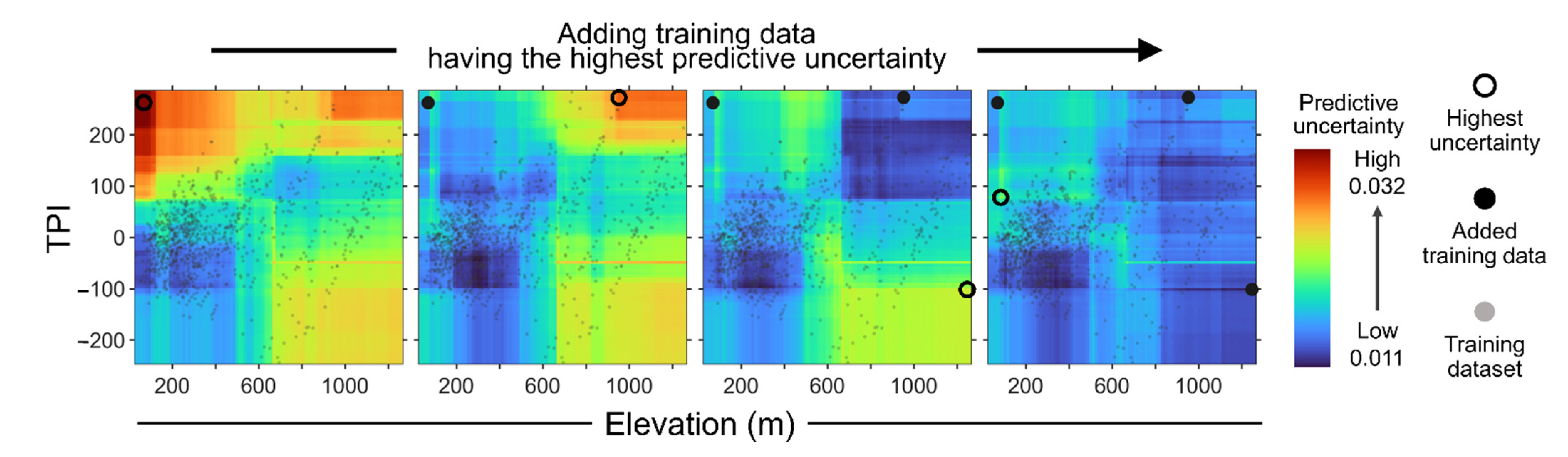
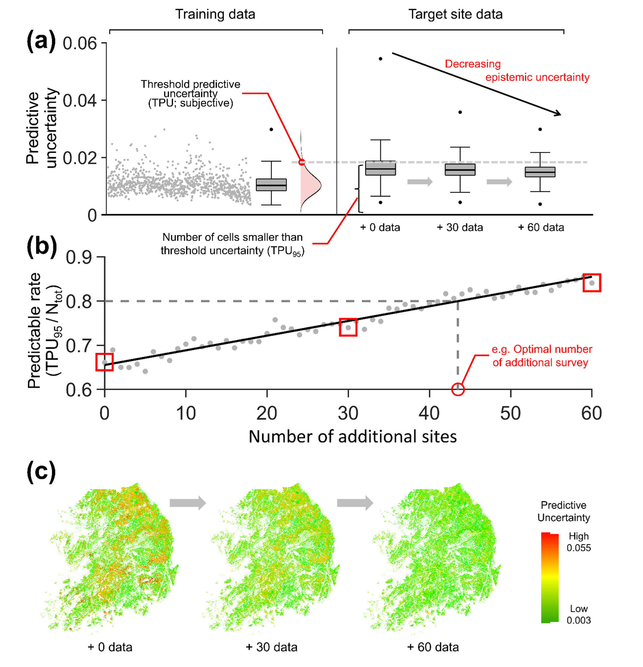
3.5. Our Simple Optimal Sampling Algorithm

A simple optimal sampling algorithm was developed based on the relationship between predictive uncertainty and the training dataset. Firstly, a machine learning model was developed by searching for an optimal hyperparameter set based on the collected data. The predictive uncertainty of the training set was adopted as the threshold predictive uncertainty (TPU), which will be a criterion for determining the sample size. It is determined based on the predictive uncertainty distribution of the training data used when an RF model was developed. Subsequently, the predictive uncertainties of the target site were calculated using environmental covariate data. At this point, the coordinate corresponding to the soil with the highest predictive uncertainty becomes an additional sample site. Afterward, the RF model predicts the FC value of the additional sample site, and an error term is added to the predicted value (see Appendix A). An RF model was then trained based on new training data, where a new hypothetical soil sample was added. The above process was then repeated, and additional sample sites were selected one by one. The optimal sample size was then determined based on the predictable rate, a ratio of the number of cells smaller than the TPU to the total number of grid cells.

Using this new algorithm, we selected additional sample sites to enhance the existing DSM of South Korea. The E14-S0 predictor set hierarchy-based RF model was trained using 953 collected soil samples. Afterward, we calculated the predictive uncertainty distribution using the same 953 soil samples (Figure 9a). TPU was determined using the 95th-percentile value of predictive uncertainties. Note that 95% is a subjectively selected ratio and may vary depending on the research or business purpose. Then, the environmental covariate information from a 100 m × 100 m grid of forests across South Korea was used for target data. The predictive uncertainty of each grid cell was calculated based on the developed model, and the cell with the highest uncertainty was selected as an additional study site. Afterward, updating the model and selecting additional survey sites was repeated while including additional data in the training dataset.

The predictive uncertainty gradually decreased as additional survey sites were selected (Figure 9a). If the predictive uncertainty of grid cells is less than the TPU, it can be assumed that the training dataset already contains information from those grid cells. Thus, the ratio of the number of cells smaller than the TPU (TPU₉₅) to the total number of grid cells in the target site (N_tot) was calculated to determine the predictable rate (TPU₉₅/N_tot). It was found that this rate increased with the number of additional sites (Figure 9b). Furthermore, it was confirmed that 43 additional samplings were needed if the research goal was to explain more than 80% of the target area. Additionally, the predictive uncertainty of forests nationwide decreased as optimal sampling sites were added through the sampling algorithm (Figure 9c).

We only used the training dataset’s predictive uncertainty to select the TPU. This is because if we develop a model to estimate FC through the training dataset and estimate FC using the same training dataset consecutively, the predictive uncertainty calculated at this time will be caused by the following reasons: potential errors introduced from soil collection, laboratory work, or incorrect geographical information. These factors pose irreducible uncertainty in the current situation. In other words, it is a natural variation that occurs equally, even if more soil samples are collected. Thus, the TPU was calculated based on the training dataset.

Predictive uncertainty can be primarily divided into aleatoric and epistemic uncertainties. Aleatoric (statistical) uncertainty refers to the variability of the results caused by naturally occurring random effects [40,41]. Epistemic (systematic) uncertainty pertains to the lack of epistemic conditions applied by analysts [42]. Thus, aleatoric uncertainty is the non-reducible type, and epistemic uncertainty is reducible [43]. Hence, the TPU set, when used as the standard, predictable rate in this study, has the characteristic of irreducible aleatoric uncertainty. In contrast, predicting the FC of target site data contains not only the epistemic uncertainty related to out-of-distribution data that were not used when the model was trained but also aleatoric uncertainty. Therefore, the model learns the corresponding soil information if new sample sites that did not exist before are added to the training dataset over time. As a result, the epistemic uncertainty steadily reduces.

This sampling algorithm is useful for collecting soils with characteristics that were not previously collected by suggesting the locations and sample size of the sample sites in a simple way using machine learning. Therefore, it can make our understanding of the explanation of FC more concrete. However, this requires future work. South Korea has started an R&D project to collect additional forest soil samples. Thus, it is necessary to verify whether the predictive uncertainty is reduced by checking the ground truth as we increase the model’s prediction performance throughout this project. Notably, collecting new samples is not the only method for enhancing DSM. A more enhanced model that can predict the FC of forest soil could be developed if additional predictors that can better explain FC are found in the future (using datasets from satellites or drones). Further, new machine learning structures are being developed to describe FC characteristics effectively.

4. Conclusions

Nine hundred and fifty-three forest soil samples and four geographical big datasets were used to develop FC predictive models. The predictive performance of four machine learning algorithms was compared, and tree-based models (RF and GB) showed a higher NSE and smaller RMSE; that is, they performed better than the other machine learning models (KNN and MLP). Therefore, RF and GB models are suitable when treating the geographically referenced big datasets of South Korea. Variable importance analysis confirmed that sand and OM as soil properties, and elevation and TPI as environmental covariates, were important variables for predicting FC. We established a different six-predictor set since data coverage varies by location across the nation. Further, considering the variable importance of soil properties and environmental covariates, machine learning models were paired with their optimal predictor set hierarchies (RF: E4-S0, E12-S0, and E14-S0; GB: E0-S4, E14-S2, and E14-S4). The FCs of South Korea were predicted using the developed models and were primarily distributed along the Baekdudaegan watershed crest line.

There was a strong relationship between model predictive uncertainties (the coefficient of variation of predicted FCs) and training data distribution. Further, we confirmed that higher uncertainties were distributed in the data scarcity area. Changes in predictive uncertainties were simulated to verify the relationship between training data scarcity and predictive uncertainty. Predictive uncertainties decreased when additional sample sites were added to the training dataset. To determine the optimal sample sites to strengthen DSM in South Korea, environmental covariate information of each grid cell (raster with a cell size of 100 m) was used. A grid cell with the highest predictive uncertainty was selected as a new sample site. Geographical information of the new sample site was added to the training dataset, and the site selection process was iterated. Epistemic uncertainty decreased when new sample sites were added to the training dataset. The sample size was determined using the predictable rate, calculated by the total number of grid cells in the target site and a TPU that is subjectively established. When the TPU was decided using the 95th-percentile value of predictive uncertainties, 80% of the target area could be successfully explained when 43 optimal sample sites were added to the existing datasets. This intuitive sampling design can be generalized to coordinate the sampling sites and determine the sampling size for strengthening DSM.

References

1. Branger, F.; McMillan, H.K. Deriving hydrological signatures from soil moisture data. Hydrol. Process. 2020, 34, 1410–1427. [Google Scholar] [CrossRef]
2. Krause, P.; Bäse, F.; Bende-Michl, U.; Fink, M.; Flügel, W.; Pfennig, B. Multiscale investigations in a mesoscale catchment—Hydrological modelling in the Gera catchment. Adv. Geosci. 2006, 9, 53–61. [Google Scholar] [CrossRef] [Green Version]
3. McKenzie, N.J.; Austin, M.P. A quantitative Australian approach to medium and small scale surveys based on soil stratigraphy and environmental correlation. Geoderma 1993, 57, 329–355. [Google Scholar] [CrossRef]
4. Piikki, K.; Wetterlind, J.; Söderström, M.; Stenberg, B. Perspectives on validation in digital soil mapping of continuous attributes—A review. Soil Use Manag. 2021, 37, 7–21. [Google Scholar] [CrossRef]
5. Chen, H.; Chen, J.; Ding, J. Data Evaluation and Enhancement for Quality Improvement of Machine Learning. IEEE Trans. Reliab. 2021, 70, 831–847. [Google Scholar] [CrossRef]
6. Hagendorff, T. Linking Human and Machine Behavior: A New Approach to Evaluate Training Data Quality for Beneficial Machine Learning. Minds Mach. 2021, 31, 563–593. [Google Scholar] [CrossRef] [PubMed]
7. De Gruijter, J.J.; McBratney, A.B.; Minasny, B.; Wheeler, I.; Malone, B.P.; Stockmann, U. Farm-scale soil carbon auditing. Geoderma 2016, 265, 120–130. [Google Scholar] [CrossRef]
8. Domburg, P.; de Gruijter, J.J.; Brus, D.J. A structured approach to designing soil survey schemes with prediction of sampling error from variograms. Geoderma 1994, 62, 151–164. [Google Scholar] [CrossRef]
9. Walvoort, D.J.J.; Brus, D.J.; de Gruijter, J.J. An R package for spatial coverage sampling and random sampling from compact geographical strata by k-means. Comput. Geosci. 2010, 36, 1261–1267. [Google Scholar] [CrossRef]
10. Brus, D.J. Sampling for digital soil mapping: A tutorial supported by R scripts. Geoderma 2019, 338, 464–480. [Google Scholar] [CrossRef]
11. Yang, H.; Yoo, H.; Lim, H.; Kim, J.; Choi, H.T. Impacts of Soil Properties, Topography, and Environmental Features on Soil Water Holding Capacities (SWHCs) and Their Interrelationships. Land 2021, 10, 1290. [Google Scholar] [CrossRef]
12. Alifu, H.; Vuillaume, J.F.; Johnson, B.A.; Hirabayashi, Y. Machine-learning classification of debris-covered glaciers using a combination of Sentinel-1/-2 (SAR/optical), Landsat 8 (thermal) and digital elevation data. Geomorphology 2020, 369, 107365. [Google Scholar] [CrossRef]
13. Araya, S.N.; Ghezzehei, T.A. Using Machine Learning for Prediction of Saturated Hydraulic Conductivity and Its Sensitivity to Soil Structural Perturbations. Water Resour. Res. 2019, 55, 5715–5737. [Google Scholar] [CrossRef]
14. Lawrence, R. Classification of remotely sensed imagery using stochastic gradient boosting as a refinement of classification tree analysis. Remote Sens. Environ. 2004, 90, 331–336. [Google Scholar] [CrossRef]
15. Lee, J.; Lee, S.; Hong, J.; Lee, D.; Bae, J.H.; Yang, J.E.; Kim, J.; Lim, K.J. Evaluation of Rainfall Erosivity Factor Estimation Using Machine and Deep Learning Models. Water 2021, 13, 382. [Google Scholar] [CrossRef]
16. Yang, T.; Zhang, L.; Kim, T.; Hong, Y.; Zhang, D.; Peng, Q. A large-scale comparison of Artificial Intelligence and Data Mining (AI&DM) techniques in simulating reservoir releases over the Upper Colorado Region. J. Hydrol. 2021, 602, 126723. [Google Scholar]
17. Breiman, L. Random Forests. Mach. Learn. 2001, 45, 5–32. [Google Scholar] [CrossRef] [Green Version]
18. Breiman, L. Bagging predictors. Mach. Learn. 1996, 24, 123–140. [Google Scholar] [CrossRef] [Green Version]
19. Zhang, M.; Shi, W.; Xu, Z. Systematic comparison of five machine-learning models in classification and interpolation of soil particle size fractions using different transformed data. Hydrol. Earth Syst. Sci. 2020, 24, 2505–2526. [Google Scholar] [CrossRef]
20. Motevalli, A.; Naghibi, S.A.; Hashemi, H.; Berndtsson, R.; Pradhan, B.; Gholami, V. Inverse method using boosted regression tree and k-nearest neighbor to quantify effects of point and non-point source nitrate pollution in groundwater. J. Clean. Prod. 2019, 228, 1248–1263. [Google Scholar] [CrossRef]
21. Mansuy, N.; Thiffault, E.; Paré, D.; Bernier, P.; Guindon, L.; Villemaire, P.; Poirier, V.; Beaudoin, A. Digital mapping of soil properties in Canadian managed forests at 250m of resolution using the k-nearest neighbor method. Geoderma 2014, 235, 59–73. [Google Scholar] [CrossRef]
22. Subasi, A. EEG signal classification using wavelet feature extraction and a mixture of expert model. Expert Syst. Appl. 2007, 32, 1084–1093. [Google Scholar] [CrossRef]
23. Périé, C.; Ouimet, R. Organic carbon, organic matter and bulk density relationships in boreal forest soils. Can. J. Soil Sci. 2008, 88, 315–325. [Google Scholar] [CrossRef]
24. Prévost, M. Predicting Soil Properties from Organic Matter Content following Mechanical Site Preparation of Forest Soils. Soil Sci. Soc. Am. J. 2004, 68, 943–949. [Google Scholar] [CrossRef]
25. Huynh-Thu, V.A.; Irrthum, A.; Wehenkel, L.; Geurts, P. Inferring regulatory networks from expression data using tree-based methods. PLoS ONE 2010, 5, e12776. [Google Scholar] [CrossRef]
26. Altmann, A.; Toloşi, L.; Sander, O.; Lengauer, T. Permutation importance: A corrected feature importance measure. Bioinformatics 2010, 26, 1340–1347. [Google Scholar] [CrossRef] [PubMed] [Green Version]
27. Zhang, Y.; Schaap, M.G.; Zha, Y. A High-Resolution Global Map of Soil Hydraulic Properties Produced by a Hierarchical Parameterization of a Physically Based Water Retention Model. Water Resour. Res. 2018, 54, 9774–9790. [Google Scholar] [CrossRef] [Green Version]
28. Myles, A.J.; Feudale, R.N.; Liu, Y.; Woody, N.A.; Brown, S.D. An introduction to decision tree modeling. J. Chemom. 2004, 18, 275–285. [Google Scholar] [CrossRef]
29. Hu, L.Y.; Huang, M.W.; Ke, S.W.; Tsai, C.F. The distance function effect on k-nearest neighbor classification for medical datasets. SpringerPlus 2016, 5, 1304. [Google Scholar] [CrossRef] [PubMed] [Green Version]
30. Brouwer, R.K. A feed-forward network for input that is both categorical and quantitative. Neural Netw. 2002, 15, 881–890. [Google Scholar] [CrossRef]
31. Okada, S.; Ohzeki, M.; Taguchi, S. Efficient partition of integer optimization problems with one-hot encoding. Sci. Rep. 2019, 9, 13036. [Google Scholar] [CrossRef] [PubMed]
32. Aldrees, A.; Nachabe, M. Capillary Length and Field Capacity in Draining Soil Profiles. Water Resour. Res. 2019, 55, 4499–4507. [Google Scholar] [CrossRef]
33. Lal, R. Soil Organic Matter and Water Retention. Agron. J. 2020, 112, 3265–3277. [Google Scholar] [CrossRef]
34. Hudson, B.D. Soil Organic Matter and Available Water Capacity. J. Soil Water Conserv. 1994, 49, 189–194. [Google Scholar]
35. Rizinjirabake, F.; Tenenbaum, D.E.; Pilesjö, P. Data for Assessment of Soil Water Extractable and Percolation Water Dissolved Organic Carbon in Watersheds. Data Brief. 2019, 27, 104779. [Google Scholar] [CrossRef] [PubMed]
36. Puckett, W.E.; Dane, J.H.; Hajek, B.F. Physical and Mineralogical Data to Determine Soil Hydraulic Properties. Soil Sci. Soc. Am. J. 1985, 49, 831–836. [Google Scholar] [CrossRef]
37. Purushothaman, N.K.; Reddy, N.N.; Das, B.S. National-Scale Maps for Soil Aggregate Size Distribution Parameters Using Pedotransfer Functions and Digital Soil Mapping Data Products. Geoderma 2022, 424, 116006. [Google Scholar] [CrossRef]
38. Lim, H.; Yang, H.; Chun, K.W.; Choi, H.T. Development of Pedo-Transfer Functions for the Saturated Hydraulic Conductivity of Forest Soil in South Korea Considering Forest Stand and Site Characteristics. Water 2020, 12, 2217. [Google Scholar] [CrossRef]
39. Sun, J.; Lang, J.; Fujita, H.; Li, H. Imbalanced Enterprise Credit Evaluation with DTE-SBD: Decision Tree Ensemble Based on SMOTE and Bagging with Differentiated Sampling Rates. Inf. Sci. 2018, 425, 76–91. [Google Scholar] [CrossRef]
40. Hüllermeier, E.; Waegeman, W. Aleatoric and Epistemic Uncertainty in Machine Learning: An Introduction to Concepts and Methods. Mach. Learn. 2021, 110, 457–506. [Google Scholar] [CrossRef]
41. Senge, R.; Bösner, S.; Dembczyński, K.; Haasenritter, J.; Hirsch, O.; Donner-Banzhoff, N.; Hüllermeier, E. Reliable Classification: Learning Classifiers that Distinguish Aleatoric and Epistemic Uncertainty. Inf. Sci. 2014, 255, 16–29. [Google Scholar] [CrossRef] [Green Version]
42. Hofer, E.; Kloos, M.; Krzykacz-Hausmann, B.; Peschke, J.; Woltereck, M. An Approximate Epistemic Uncertainty Analysis Approach in the Presence of Epistemic and Aleatory Uncertainties. Reliab. Eng. Syst. Saf. 2002, 77, 229–238. [Google Scholar] [CrossRef]
43. Wang, G.; Li, W.; Aertsen, M.; Deprest, J.; Ourselin, S.; Vercauteren, T. Aleatoric Uncertainty Estimation with Test-Time Augmentation for Medical Image Segmentation with Convolutional Neural Networks. Neurocomputing 2019, 338, 34–45. [Google Scholar] [CrossRef] [PubMed]
Figure 1. (a) South Korea’s global location and (b) its 953 forest soil sampling sites.
Land 11 02098 g001
Figure 2. (a) Distribution of forest soils used in this study (953 soil samples) across USDA textural classes and (b) mean values and standard deviations of FC and soil texture class (STC) percentages.
Land 11 02098 g002
Figure 3. Comparison of machine learning model performance. Two tree-based models, GB and RF, showed higher performance than the others. KNN, k-nearest neighbors; MLP, multilayer perceptron; NSE, Nash–Sutcliffe model efficiency; RMSE, root mean-squared error.
Land 11 02098 g003
Figure 4. (a) The variable importance of each predictor, and (b) the summation variable importance of soil properties and environmental covariates for predicting FC. Variable importance was suggested using the permutation importance of GB and RF models, and feature importance was suggested for RF.
Land 11 02098 g004
Figure 5. Relationship between measured and predicted field capacities according to the six predictor set hierarchies. Training sets are plotted with gray points, and test sets are plotted in yellow-to-blue. Five-fold cross-validation was performed for model performance with the (a) E4-S0-based RF, (b) E12-S0-based RF, (c) E14-S0-based RF, (d) E0-S4-based GB, (e) E14-S2-based GB, and (f) E14-S4-based GB models.
Land 11 02098 g005
Figure 6. Spatial distribution of predicted forest FCs on a national scale.
Land 11 02098 g006
Figure 7. A 2D heatmap of (a,d) predicted FCs and (b,e) predictive uncertainties, which are the standardized mean values of the CV, and (c,f) scatterplot of the training set. The distribution of the predicted uncertainties is not related to the predicted FCs but is strongly related to the distribution of the training set.
Land 11 02098 g007
Figure 8. Examples of adding training data and changes in predictive uncertainties. Predictive uncertainties decreased when additional training data were used. Note that the 2D imaginary soils used in this simulation had the same characteristics, apart from the two variables of interest (elevation and TPI), which makes the predictive uncertainty reduction appear radical.
Land 11 02098 g008
Figure 9. Selecting optimal sampling sites to strengthen the DSM of South Korea using the optimal sampling algorithm suggested in this study. A predictive model was developed with 953 training data items. (a) Threshold predictive uncertainty was determined by the distribution of the predictive uncertainty when using the training data as input to the developed model. Epistemic uncertainty decreased with the addition of training data. We do not show all outliers in the box plot, and only the maximum and minimum values of the dataset are indicated. (b) The predictable rate increased according to the number of additional sites, which helped to confirm the optimal number of additional survey sites. (c) Expected results of the spatial distribution of predictive uncertainty in South Korea are shown when 30 and 60 data items are collected using the optimal sampling algorithm. Ntot, number of grid cells in the target site.
Land 11 02098 g009