Article

Agricultural Land Abandonment in Bulgaria: A Long-Term Remote Sensing Perspective, 1950–1980

by
Mustafa Erdem Kabadayı
1,2,*,
Paria Ettehadi Osgouei
1,3 and
Elif Sertel
1,4
1
Department of History, Koç University, Istanbul 34450, Turkey
2
School of Geographical and Earth Sciences, University of Glasgow, Glasgow G12 8QQ, UK
3
Institute of Informatics, Department of Communication Systems, Istanbul Technical University, Istanbul 34469, Turkey
4
Faculty of Civil Engineering, Geomatics Engineering Department, Istanbul Technical University, Istanbul 34469, Turkey
*
Author to whom correspondence should be addressed.
Land 2022, 11(10), 1855; https://doi.org/10.3390/land11101855
Submission received: 1 October 2022 / Revised: 16 October 2022 / Accepted: 18 October 2022 / Published: 20 October 2022
(This article belongs to the Special Issue Modeling Land Use Change Using Historical and Archaeological Datasets)

Abstract

:
Agricultural land abandonment is a globally significant threat to the sustenance of economic, ecological, and social balance. Although the driving forces behind it can be multifold and versatile, rural depopulation and urbanization are significant contributors to agricultural land abandonment. In our chosen case study, focusing on two locations, Ruen and Stamboliyski, within the Plovdiv region of Bulgaria, we use aerial photographs and satellite imagery dating from the 1950s until 1980, in connection with official population census data, to assess the magnitude of agricultural abandonment for the first time from a remote sensing perspective. We use multi-modal data obtained from historical aerial and satellite images to accurately identify Land Use Land Cover changes. We suggest using the rubber sheeting method for the geometric correction of multi-modal data obtained from aerial photos and Key Hole missions. Our approach helps with precise sub-pixel alignment of related datasets. We implemented an iterative object-based classification approach to accurately map LULC distribution and quantify spatio-temporal changes from historical panchromatic images, which could be applied to similar images of different geographical regions.

1. Introduction

Agricultural land abandonment has been a significant land use change, attracting increased global attention since the 2010s [1]. It has been a concern for the European Union, as it has been forecasted that 11% of agricultural land in the EU is at a high risk of abandonment by 2030 [2]. The Common Agricultural Policy (CAP) has further accelerated the dual process of intensification of agriculture and agricultural land abandonment in the EU [3]. This political context and ecological momentum have facilitated large-scale EU-wide agricultural land abandonment examinations [4,5,6], including predictions and modelings for the near future [5,7,8]. Earth observation (EO) data, collected from various satellite platforms (starting in the 1970s with the Landsat program) and processed with remote sensing methods, has been a crucial and ever-developing aspect of these research efforts. In the last decades, for several local scale case studies, earlier monochromatic visual material (starting from the 1940s aerial photographs and the 1960s satellite imagery) has also been incorporated into Land Use Land Cover Changes (LULCC) examinations for more extended periods [9,10,11,12]. There have also been attempts to include historical cadastral maps as even earlier datasets, and in combination with aerial photographs [13,14,15,16,17].
We aim to quantitively analyze the land abandonment problem using very high-resolution (VHR) historical aerial and satellite images with image processing techniques. Our study examines the agricultural land abandonment problem following remote sensing methodologies using panchromatic visual material consisting of aerial photographs and satellite imagery from the Key Hole (KH) program between the 1950s and the 1980s. Our methodological strength is making joint use of historical population censuses in combination with the concepts of rural depopulation and urbanization in addition to our relatively older remote sensing data. For the specific dynamics of agricultural land abandonment in Bulgaria and the selected two locations, covering around 30 years with five cross-sections before the 1990s is advantageous. The 1950s preceded radical rural depopulation and urbanization, which we observe in Bulgaria in the later years of our research period. Rural depopulation and urbanization are significant pull and push factors for populated places, resulting in agricultural land abandonment on both population gaining and losing ends. Rural depopulation poses a substantial threat to demographic and economic stability and is an emerging research field [18]. It has also been studied in connection to agricultural land abandonment from a remote sensing perspective using aerial photographs and satellite imagery for other countries in the EU [12,19,20,21].
To our knowledge, agricultural land abandonment or rural depopulation in Bulgaria has not been studied from a remote sensing perspective, if we leave aside our preliminary work [22,23] and a follow-up study inspired and shaped by our work to a more considerable extent than it has been mentioned in acknowledgement [24]. These studies were also limited to their early satellite imagery. They do not go back to the 1940s or the 1950s, and they do not conduct an examination of LULCC in correlation with demographic change, as we intend here. Bulgaria is an interesting case study to examine LULCC in the long run. Not only because of the drastic impact of the collapse of the Soviet Union in east and southeast Europe in general [25], but specifically, first due to a relatively late establishment of the communist rule and following drastic political changes in land regime, such as radical collectivization starting in the 1940s and peaking in the 1950s, [26] and secondly to a relative late accession to the EU in 2007 and with an ongoing heavy reliance on the agricultural sector. Nevertheless, few existing remote sensing studies on LULC for Bulgaria [27,28,29,30] have hardly a long-term perspective and do not address rural depopulation.
Rural depopulation is a massive threat to Bulgarian demography, and even to cultural heritage [31], especially in the transitional period after 1989 [32], which badly hit rural areas starting from the 1970s [33,34]. The rural depopulation of Bulgaria has been recently mapped for the period after the fall of communism [35], but has not been examined from a remote sensing perspective until now.
This study proposes an iterative geographic object-based image analysis (GeOBIA) approach to accurately determine historical LULCC using panchromatic aerial photographs and satellite images. A detailed examination of the dynamics behind the detected LULCC is beyond the goal setting of this preliminary study. With our devised object-based image analysis methods, we share a detailed workflow to segment historical panchromatic aerial photographs and early panchromatic satellite imagery. As end products, we create historical LULC maps using a land cover classification scheme derived from the European Space Agency (ESA) WorldCover project. In this regard, our historical land use classes are commensurable with the current, detailed, and high-resolution data created from Sentinel-1 and 2 images, and lend themselves to longitudinal dataset construction and analysis. However, within the limited scope of this article, we did not pursue these latter goals.

2. Materials and Methods

2.1. Satellite Imagery and Aerial Photographs to Examine Long-Run Land Use and Land Cover Changes

The satellite image dataset prepared for the Stamboliyski and Ruen study regions includes three images from the collections of declassified U.S. military intelligence missions from the KH optical reconnaissance satellites. We used images from Corona and Hexagon satellites operated between 1960 and 1972, and between 1971 and 1986, respectively. The archive of Corona’s declassified satellite images was released and offered for public use in February 1995 [36]. The historical data obtained from the declassified archive of US satellite imageries have been useful in several remote sensing applications, including historical LULCC [37,38,39,40,41,42,43,44,45,46,47]; however, not for Southeast Europe and not in combination with aerial photographs, except for a recent example of combining 1945 aerial photographs with 1975 Hexagon imagery for deltaic areas in Greece [48]. The follow-up Hexagon reconnaissance mission’s imagery was declassified in 2002 and 2011. Hexagon was the most sophisticated and the last film-based orbiting photo-reconnaissance satellite [49]. Although Hexagon imagery has high spatial resolution and advanced photogrammetric qualities, such as offering larger footprints without complex panoramic distortions [50], it has not been as widely used as its predecessors, such as Corona. Almost all the Hexagon project imagery taken by KH-9 system cameras with close to global coverage was declassified in 2011 (Declass-3). However, the imagery was only available at the National Archives and Records Administration (NARA) for personal inquiry until 2019, when the third phase of 14,000 declassified rolls was transferred to the USGS, EROS Center. Since then, they are gradually becoming available online for scanning and downloading (https://www.usgs.gov/centers/eros/science/usgs-eros-archive-declassified-data-declassified-satellite-imagery-3 accessed on 1 October 2022). Previously declassified and online available Hexagon imagery covered mainly parts of North America and polar regions [51].
The possible use of Hexagon data for archaeology and historical research has already been highlighted [51,52,53]. Due to its higher spatial resolution compared to early Landsat missions, despite being panchromatic, Hexagon imagery lends itself well to long-term glaciology research [50,54,55,56,57,58,59] and, to a lesser extent, historical digital elevation model constructions [60,61,62]. Most of the research used manual vectorization techniques to extract geographic information.
Historical aerial photographs have been used for LULCC in several studies [63,64], focusing on relatively small areas due to the coverage limitations of aerial photographs [65]. For over ten years, there have also been attempts to create long-term datasets by using aerial photographs and satellite imagery to examine historical LULCC [66], including our recent work, which combined historical maps with aerial photographs and modern satellite imagery [17,67]. Recently, there have also been attempts to automatize object-based image analysis of aerial photographs to conduct LULCC studies [68]. Nevertheless, as we already mentioned, using historical aerial photographs starting as early as the 1940s and the 1950s in combination with early satellite imagery to examine long-term LULCC is a rare undertaking. Furthermore, adding matching demographic data from the censuses is a novel approach to focus on rural depopulation and urban sprawl.

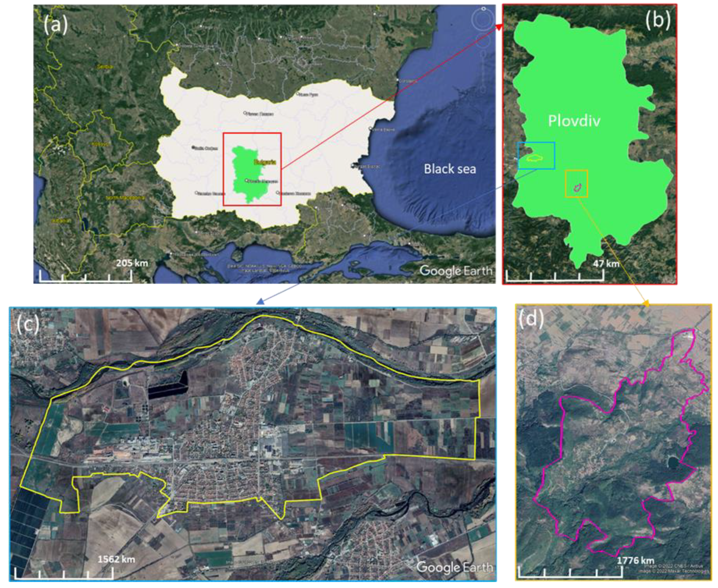
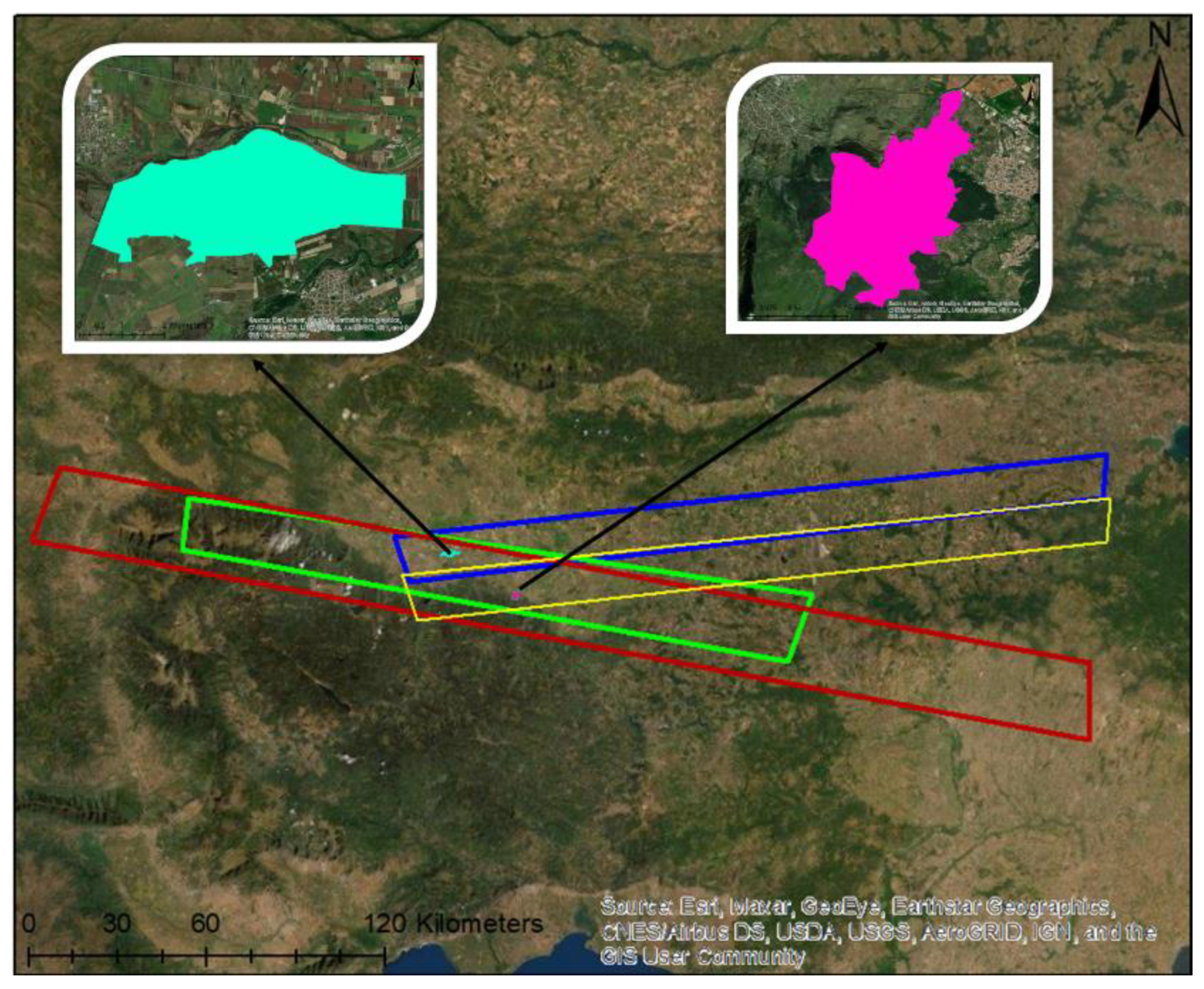
2.2. Study Areas and Datasets

We wanted to select two populated regions emphasizing two drivers of LULCC: rural depopulation and rapid population growth. Bulgaria has one of the fastest shrinking populations worldwide, and this trend is expected to continue at least until 2050 [69]. Bulgaria is in the middle of a demographic crisis on the national level. Furthermore, due to the hundreds of partially depopulated villages, it is possible to use the term demographic catastrophe at the rural level [70]. Moreover, the Plovdiv district has the country’s highest share of the rural population [71]. Therefore, we decided to focus on the Plovdiv district. Thanks to the online availability of the National Register of Populated Places of the National Statistical Institute of Bulgaria, it is possible to detect populated places with drastic demographic changes from 1934 to 2020 [72]. Every populated place is given a unique Unified Classification of Administrative-Territorial and Territorial Units (UCATTU, EKATTE in Bulgarian) number; 63238 and 51980 for Ruen and Stamboliyski, respectively. After studying the long-term demographic dynamics of populated places in the Plovdiv district, we opted for Stamboliyski and Ruen as illustrative examples of drastic demographic changes in Table 1, possibly triggering dramatic LULLC. Stamboliyski experienced rapid urbanization between 1934 and 1965, had a stagnant population between 1975 and 1992, and then the population decreased. On the other hand, Ruen is an excellent example of rural depopulation, with a constant decrease in population from 1946 to 2011. These are the demographic reasons for choosing our study areas based on our research design.
We looked for and found more candidates within the Plovdiv district with suitable demographic profiles, which could be examined for urban sprawl or rural depopulation as forms of historical LULCC. The availability of high-quality aerial and satellite imagery was our second constraint in choosing our populated regions. After successfully locating an adequate number of images of sufficient quality and at suitable intervals for Stamboliyski and Ruen, we finalized our case studies.
Our study areas are shown in Figure 1. The industrialized town of Stamboliyski, located 15 km west of Plovdiv city in South-Central Bulgaria, with an estimated population of 10,738 inhabitants at the end of 2020, represents a highly dynamic landscape over the last 70 years. The village of Ruen, located 17 km south of the city of Plovdiv, with an estimated population of 268 inhabitants in 2020, represents a relatively stable area with slow and low historical land use and land cover (LULC) change. The sizes of the Stamboliyski and Ruen study areas are about 14 km2 and 6 km2, respectively.
We acquired two panchromatic Corona images from the Key Hole 4B (KH-4B) mission from 1968, and two panchromatic Hexagon images from the Key Hole 9 (KH-9) mission from 1975 and 1980. We selected images extending over study areas (e.g., Stamboliyski and Ruen) with minimal cloud, fog, and snow cover. We purchased filmstrips of chosen Corona and Hexagon images covering our study sites through the EarthExplorer graphical user interface of the U.S. Geological Survey portal. Each Corona image file consisted of four image frames (Figure 1a–d), with 7 to 10 subsets of each Hexagon image file. We list the exact dates, file names, and satellite missions of used Corona and Hexagon images, and the total number of frames and frames of each image we used covering the Ruen and Stamboliyski study areas, in Table 2.
We present the footprints of the chosen images and the boundaries of Stamboliyski city and Ruen village in Figure 2. The Corona imageries have ground coverages of 240 by 14 km, and the Hexagon imageries have ground footprints of approximately 212 by 24 km and 262 by 26 km, from 1975 and 1980, respectively. The Stamboliyski city and Ruen village boundaries, illustrated with cyan and pink borders, are covered by the 1975 and 1980 Hexagon image shots (green and red footprints). Nevertheless, we needed two Corona images from 1968 (yellow and blue footprints) to cover Ruen and Stamboliyski (Figure 2).
Other than satellite images from declassified reconnaissance archives, we obtained monochromatic aerial photographs covering our study regions, which were acquired in 1945, 1952, 1965, and 1975. Except for the photograph covering Ruen in 1945, these aerial photographs can be obtained from the Geoportal of the Ministry of Defense of the Republic of Bulgaria (https://gis.armf.bg/ accessed on 1 October 2022). We acquired the 1945 Ruen aerial photo from the Luftbilddatenbank (https://www.luftbilddatenbank.de/ accessed on 1 October 2022), a company specializing in locating unexploded ordnance. We prepared aerial photo mosaics for two study sites for four dates 1945, 1952, 1965, and 1975, utilizing a total number of 21 aerial photographs. Detailed information about the number of aerial photographs combined to cover the study areas for the chosen years is shown in Table 3.

2.3. Data Pre-Processing

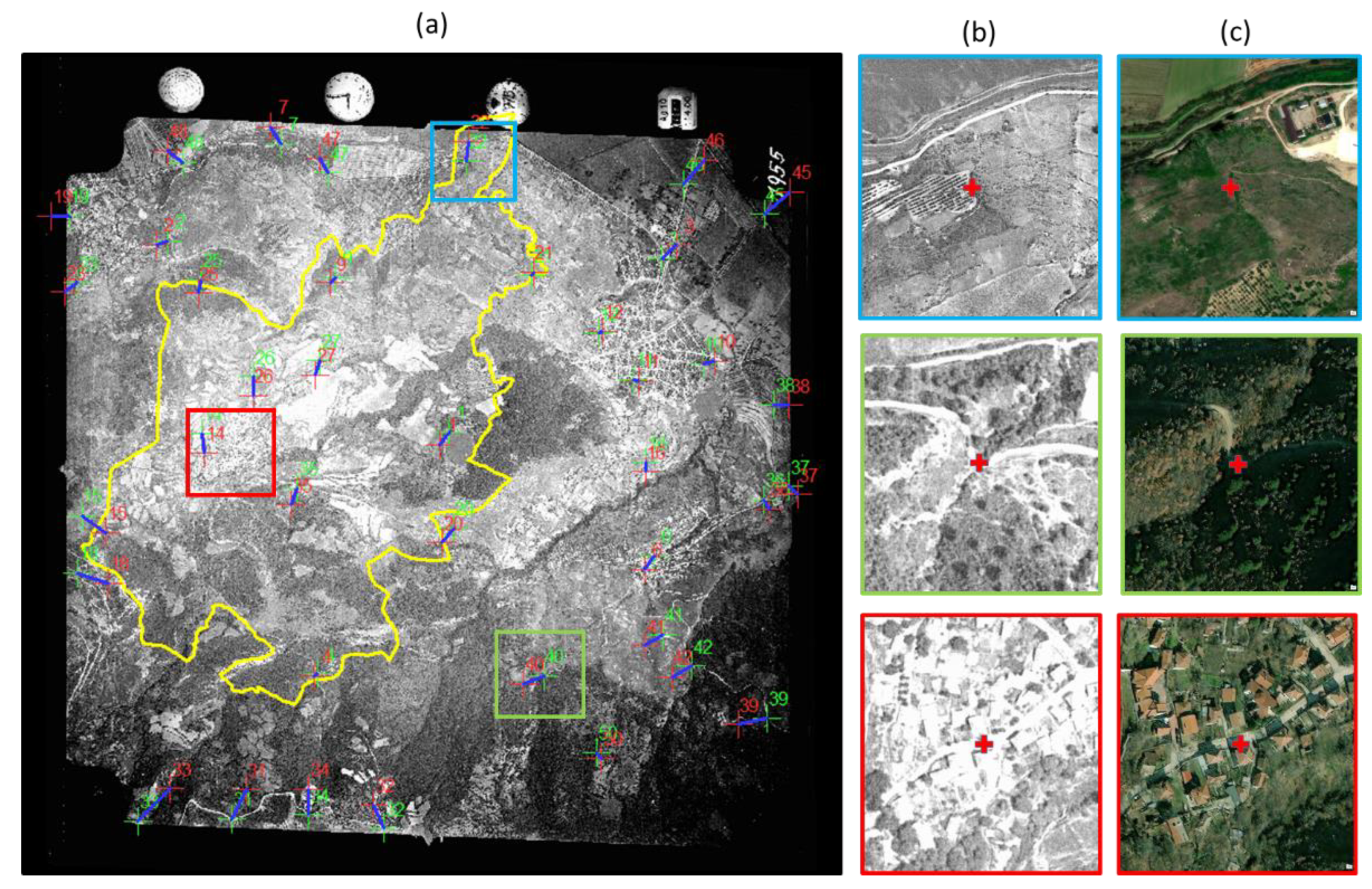
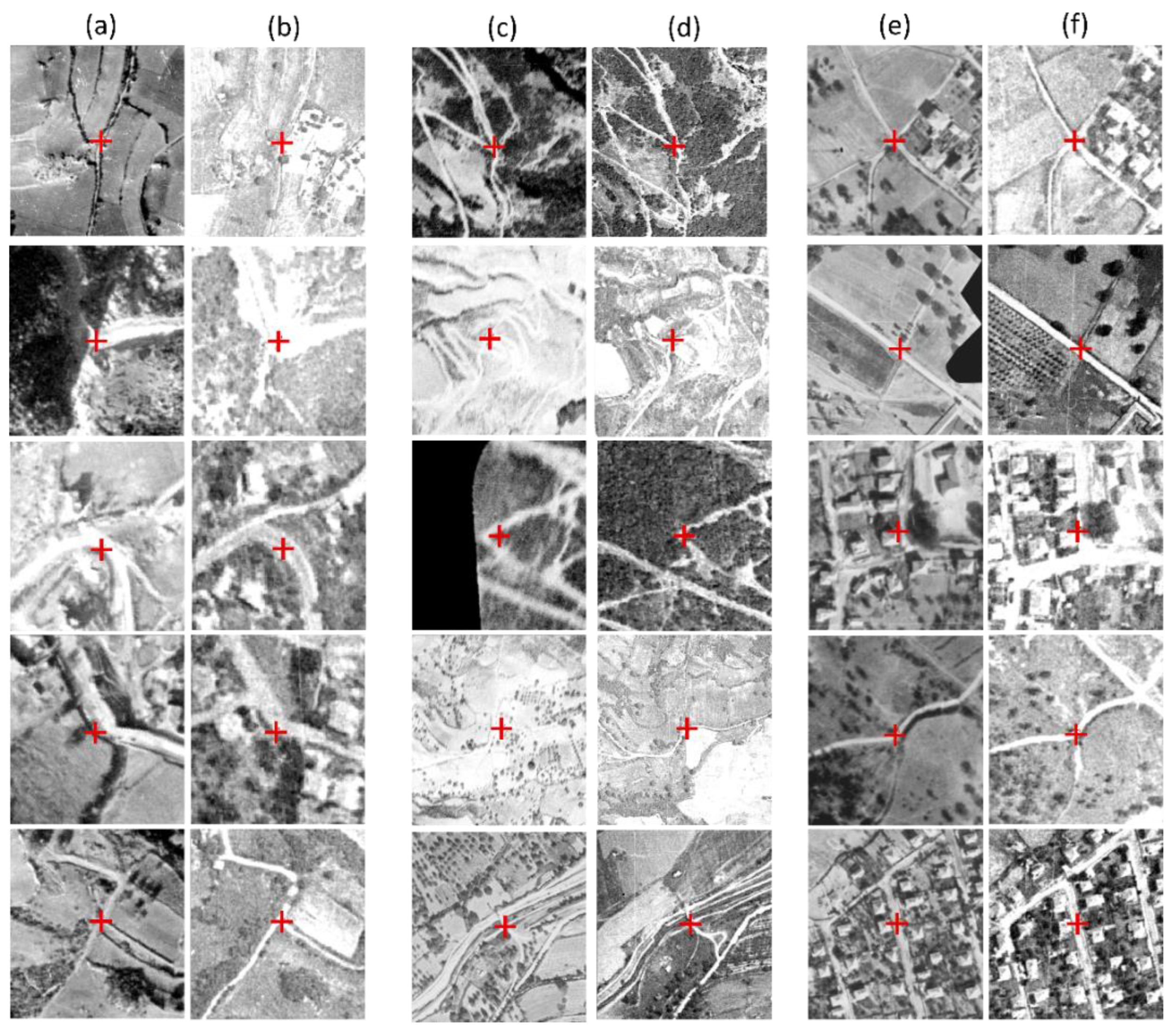
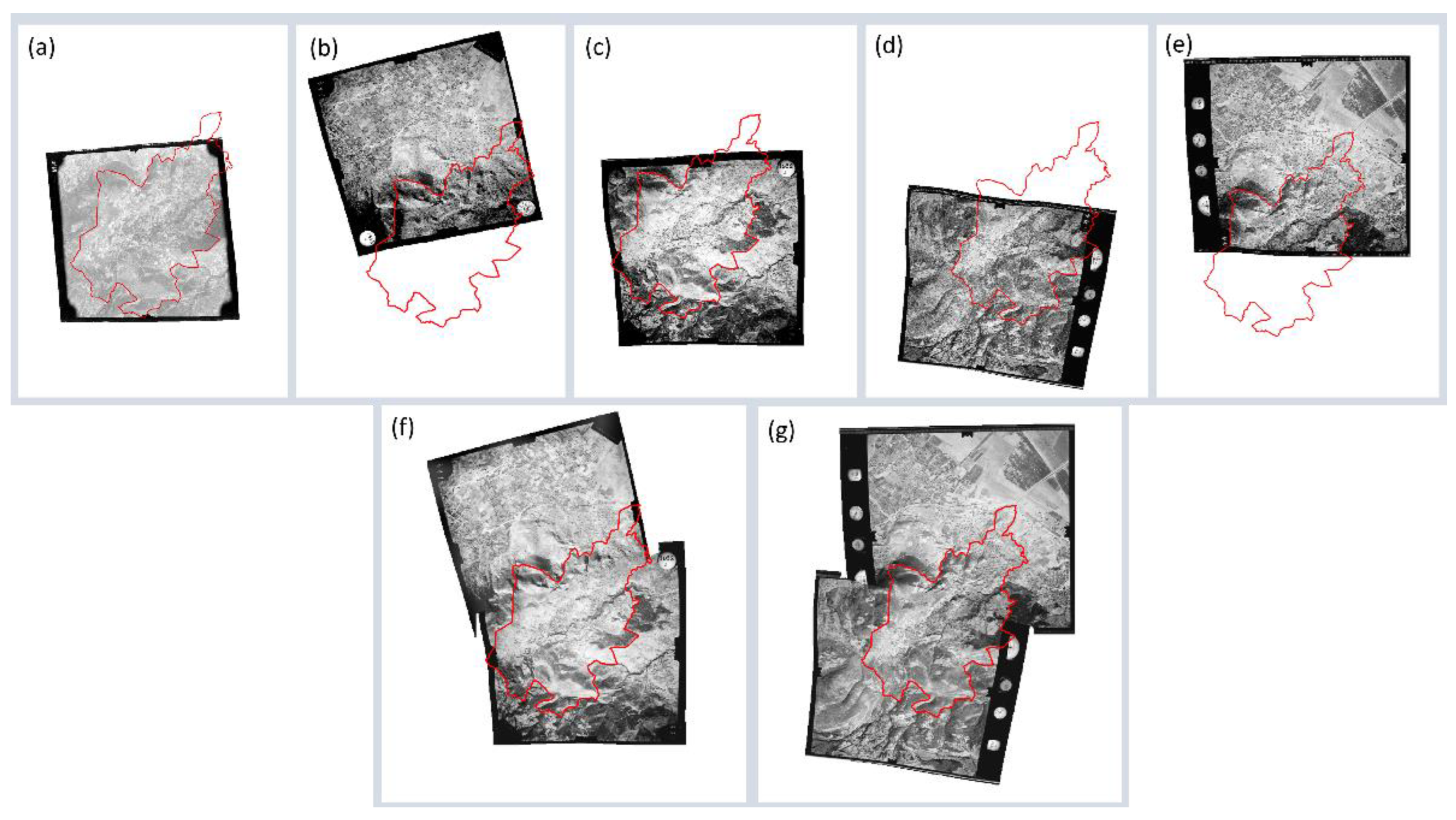
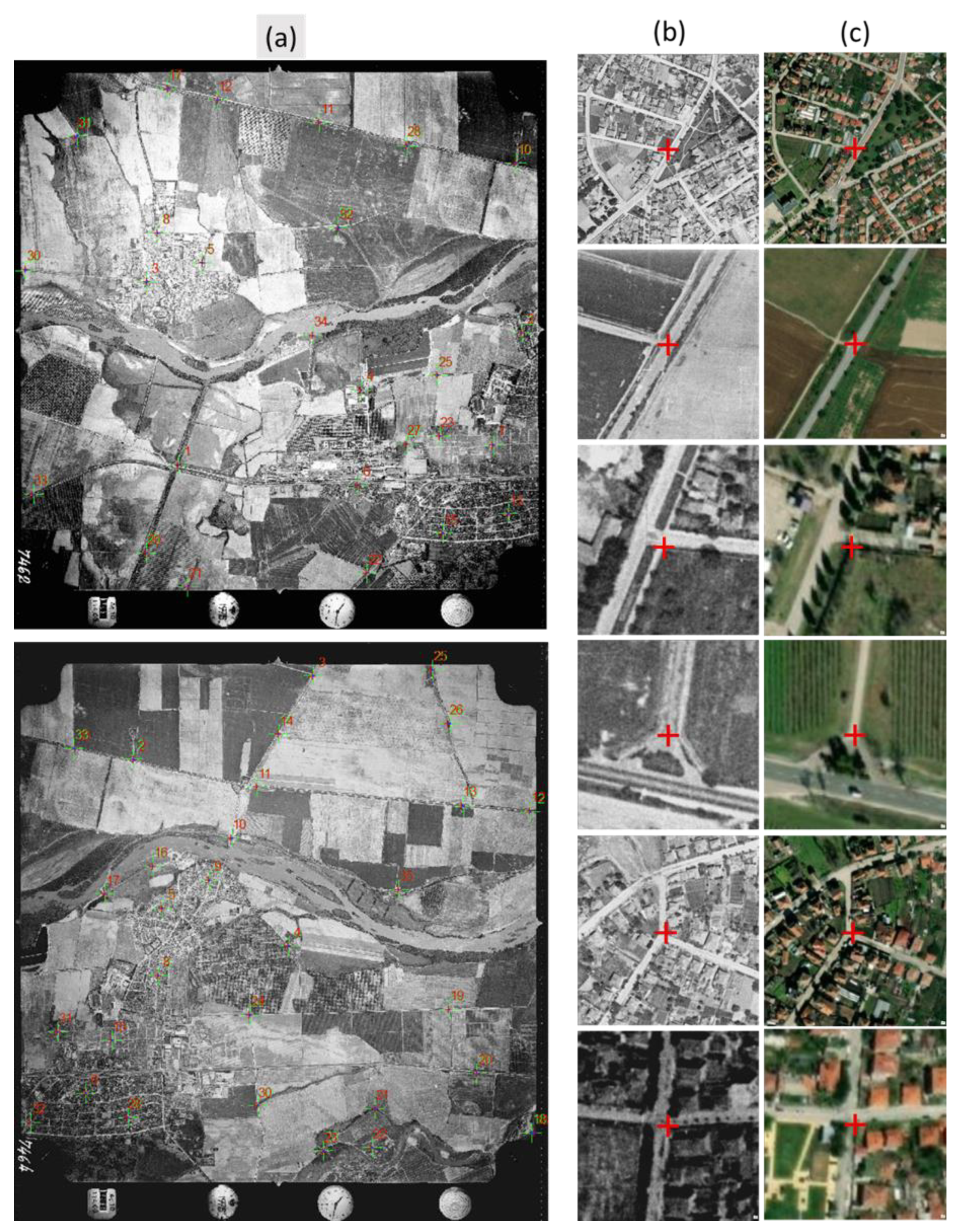
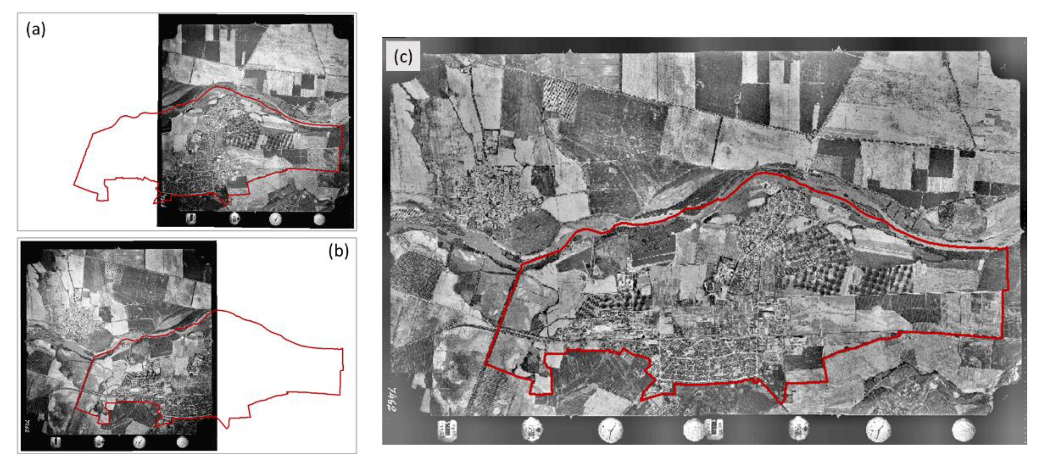
2.3.1. Geometric Correction of Aerial Photographs

To establish the correct map coordinate information for each cell in the aerial photographs, we used the spline (triangulation) transformation, a rubber sheeting method, to achieve high local accuracy [73]. Compared to polynomial functions, the spline transformation offers a very high goodness of fit to the reference data, but requires a far higher number of ground control points (GCPs) [17,74,75].
The rubber sheeting technique uses a fifth-order polynomial transformation to estimate optimal values using a mathematical function that minimizes overall surface curvature. The rubber sheeting method avoids sharp bending and provides a smooth surface that passes through the GCPs [76]. Spline-based transformations’ more comprehensive image-warping options offer better accuracy for the geometric correction of historical topographic data with positional inaccuracies and geometric distortions [77,78].
We used the georeferencing tool in ArcGIS to conduct geometric correction of multi-temporal and multi-source images. Georeferencing guarantees that satellite images and aerial photographs are correctly positioned in space, and that geometric distortion is avoided to the possible extent. Among the available datasets, we chose the one with the highest spatial resolution and widest coverage extent to be used as a reference for the further stages after conducting geometric correction using ground control points (GCPs) on the images and the Google Earth images. We chose the aerial photograph from 1975 as the reference data for the Ruen study location, since it encompasses the entire village in one frame and has a high spatial resolution. Then, we implemented a spline (triangulation) transformation to georeference the image, which provides higher accuracy for the geometric rectification of historical aerial photographs. Due to the 47 years of terrain changes between the aerial photograph from 1975 and the Google Earth image from 2021, we tried to select invariant GCPs during the period. We ensured the homogenous distribution of GCPs across the aerial photograph. Figure 3 shows the GCPs of the “1975 Ruen aerial photo”. The zoomed views of three random GCPs are also exemplified in Figure 3.
For the geometric correction of the remaining aerial photographs encompassing the Ruen village, we used the georeferenced 1975 Ruen aerial photograph defined in WGS 84 Datum and UTM Zone 35N projection as the reference. Figure 4 shows GCP samples collected from aerial photographs in 1952 and 1965, and their counterparts on a 1975 Ruen aerial photograph georeferenced at the first stage.
We created the 1952 Ruen complete aerial photograph by mosaicking the two aerial photographs covering the Ruen village. Similarly, we made the mosaicked 1965 Ruen aerial photograph. We utilized Erdas Imagine image processing program for mosaicking. Figure 5 shows aerial photographs captured in 1952 and 1965, two for each year, and the result of mosaicking these photographs into the final mosaicked images, one for each year (1952 and 1965) covering most of Ruen village boundaries.
For the Stamboliyski study region, we geometrically corrected two aerial photographs of Stamboliyski from 1975 using the GCPs collected from the Google Earth image at the first stage. Each of the aerial photographs covers an area of approximately 27 km2. Figure 6 shows the distribution of GCPs utilized for geometric correction. It presents detailed views of some random GCPs on aerial photographs from the Stamboliyski region and their counterparts on Google Earth images.
We mosaicked the geometrically-corrected aerial photographs of Stamboliyski from 1975 and used them as a reference for rectifying other aerial photographs from 1952 and 1965. Figure 7 shows the two aerial photographs of Stamboliyski from 1975 and the mosaicked aerial photograph. The red color illustrates the boundaries of the Stamboliyski town.
We then georeferenced the aerial photographs encompassing Stamboliyski from 1952 and 1965, according to the geometrically corrected and mosaicked 1975 Stamboliyski aerial photograph. We produced the 1952 Stamboliyski aerial photograph by joining five aerial photographs, each covering an area of approximately 3 km2, while three aerial photographs from 1965, each covering an area of about 12 km2, were used to mosaic the 1965 Stamboliyski aerial photograph. Figure 8 and Figure 9 show the individual aerial photographs from 1965 and 1952, respectively. Additionally, the mosaicked 1952 and 1965 aerial photographs are represented in Figure 8 and Figure 9, respectively.

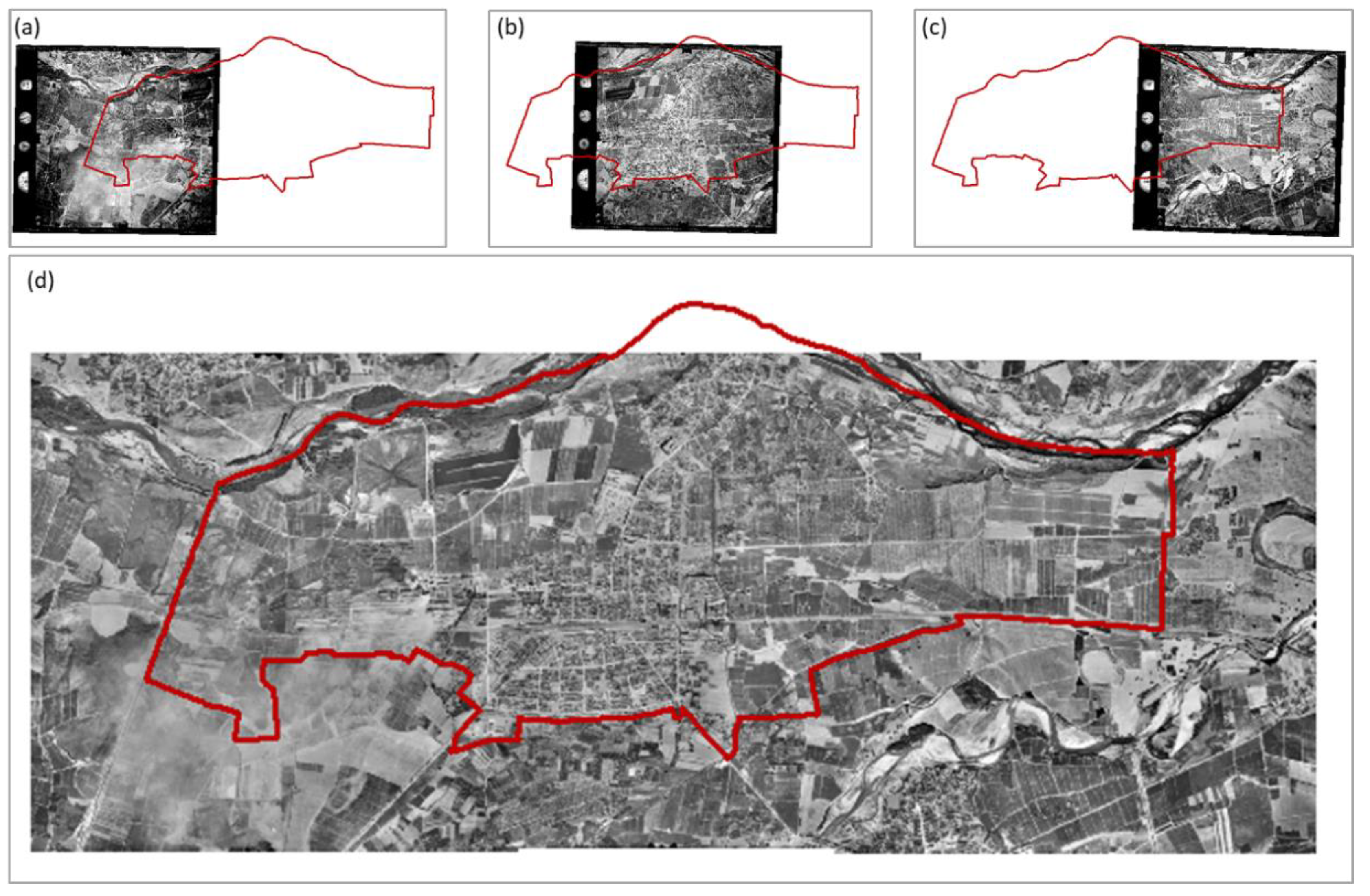
2.3.2. Geometric Correction of Satellite Images

After rectifying and mosaicking aerial photographs, we clipped the region covering Ruen and Stamboliyski from Corona and Hexagon satellite image frames, and georeferenced the clipped images according to the geometrically corrected and mosaicked 1975 Ruen and Stamboliyski aerial photograph as reference images. Figure 10 and Figure 11 present the rectified declassified images of 1968, 1975, and 1980 that encompass the Ruen and Stamboliyski borders, respectively.
We list the spatial resolutions of the rectified aerial photographs and declassified satellite images of Ruen and Stamboliyski in Table 4.
Figure 12 shows spatial resolution comparisons between aerial and satellite images of Ruen on different dates. The aerial photograph from 1945 has the highest spatial resolution, whereas the Corona image from 1968 has the lowest spatial resolution. As shown in Figure 11, buildings, roads, and even trees are detectable in satellite images and aerial photos of higher spatial resolution. At the same time, it is hard to detect buildings and borders of roads in low spatial resolution images.

2.4. Classification of Aerial and Satellite Images

We classified the geometrically-corrected aerial photographs and satellite imageries to generate the LULC maps of the two study areas. We produced eleven LULC maps, six for Ruen and five for Stamboliyski. We used aerial photos to generate the LULC maps of 1945, 1952, 1965, and 1975, and the Corona and Hexagon satellite imageries were used to form the LULC maps of 1968 and 1980.
The object-based classification approach produced better results than pixel-based approaches, and multiple studies showed that object-based classifications have significantly superior accuracy [79,80]. The OBIA technique’s segmentation step divides an image into useful image objects and meaningful entities composed of many nearby pixels. The most widely-used segmentation technique is multi-resolution segmentation (MRS) [81]. In the MRS method, a scale parameter determines the size of the resulting objects. It depends on the study area’s characteristics and the image’s spatial resolution. When a higher scale parameter value is selected, more merging is allowed, and the object is produced at a larger size.
In contrast, fine-scale values enable the formation of smaller objects. The ideal volume of a user-defined scale parameter for a study area should be set by testing the overall effect of segmentation results on object-based classification at various scales [82]. In the MRS algorithm, each pixel is considered an individual object, and pairs of image objects are combined throughout the pairwise clustering process in numerous subsequent steps in an interactive region-growing approach to generate more significant segments [83]. Merging the adjacent pixels is achieved by measuring the nearby object heterogeneity and the internal homogeneity of an object. The objects are merged until the assumption for internal homogeneity, and the threshold for surrounding object heterogeneity, are maintained. A combination of color (spectral values) and shape features make up the homogeneity criterion [84].
The objects are labeled in the second stage of the OBIA technique, known as the classification phase. The objects can be classified through the object-oriented supervised classification method, or the knowledge-based classification approach [85,86].
In the knowledge-based classification technique, the classification rules—also referred to as rule bases or knowledge models—are established and refined to identify the objects. Object identification is performed by utilizing a set of features, including texture (homogeneity, dissimilarity, entropy, contrast), shape (compactness, rectangular fit), position (distance, coordinates), extent (length/width), layer values (mean, standard deviation, mode), etc. An analyst’s knowledge of an object’s coverage, shape, texture, location, and size is utilized to determine the best threshold for the feature properties offered by e-cognition tools.

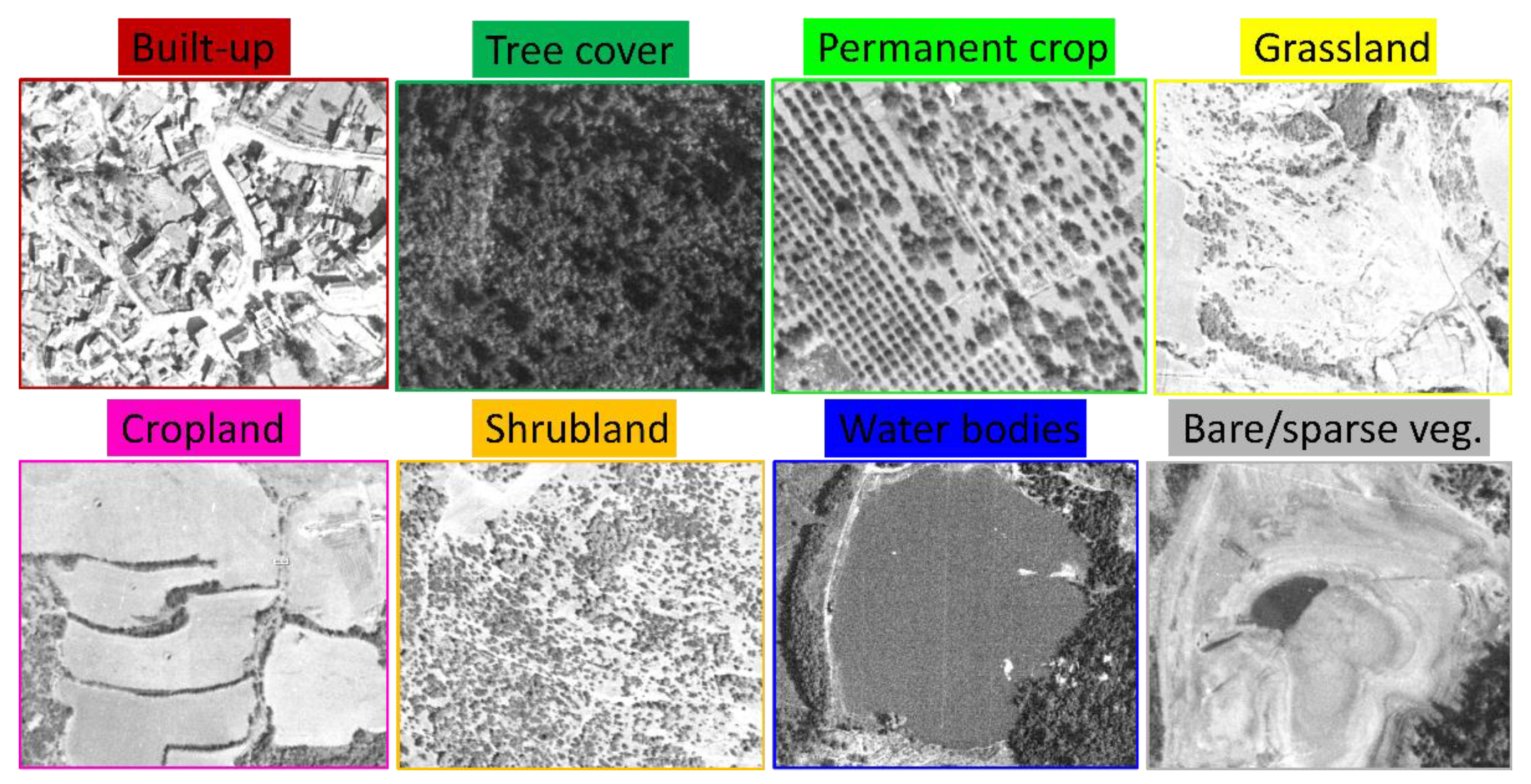
2.4.1. Classification Schema
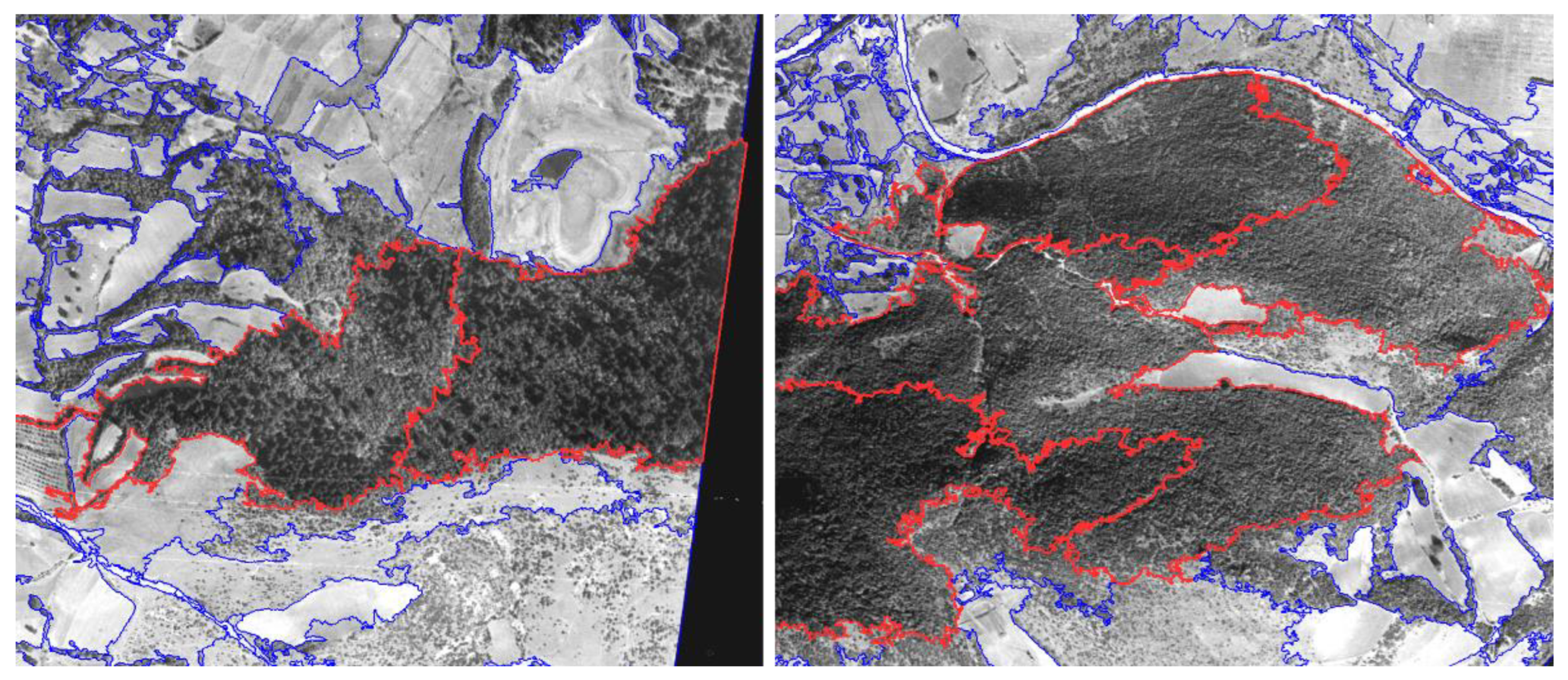
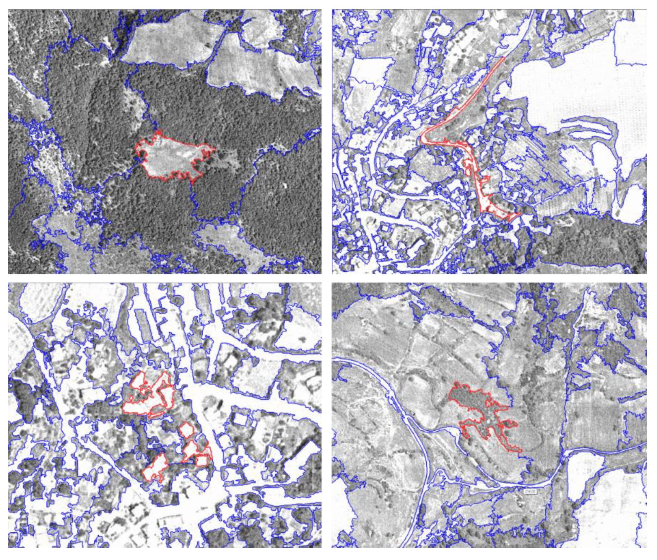
The LULC map in this study provides eight classes and is defined using the land cover classification system adopted in European Space Agency (ESA) WorldCover project. During the ESA WorldCover project, detailed and high-resolution information on worldwide LULC cover was provided by the classification of Sentinel-1 and 2 images (ESA-WorldCover, 2020). The land cover classes in our work are derived from the ESA land cover classification scheme including cropland, built-up, bare/sparse vegetation, grassland, shrubland, water bodies, and tree cover. The explanation of each land cover class can be found in “WorldCover_PUM_v1.0” (https://worldcover2020.esa.int/, accessed on 1 October 2022), and we also provide examples from aerial photographs and satellite images for each land cover class in Figure 13.
In addition to these land cover classes, we added a land cover class to our classification scheme to classify permanent cropland. In the ESA classification schema, perennial woody plants and plantations (e.g., fruit trees, nut trees, oil palm, olive trees) are classified as “tree cover”. In this study, we separated permanent cropland from forest tree cover to examine changes in the agricultural region of the study sites.

2.4.2. Methodology

We first chose one photograph for each study region with high spatial resolution, encompassing the large extent of the study areas. Then, we implemented a geographic object-based image analysis (GeOBIA) using the eCognition® program (Trimble Germany GmbH, Munich, Germany). The segmentation and classification phases of the OBIA technique are used to locate objects in an image and categorize the objects, respectively. For Ruen, the 1965 aerial photograph was the preferred image. Although the Ruen aerial photograph from 1945 has the highest resolution, the Ruen village is covered in >99% of the 1965 photograph, as opposed to only 93% in the 1945 photograph. The 1965 aerial photograph is the recommended image for Stamboliyski. Although the 1952 Stamboliyski aerial photograph has the highest resolution, the city of Stamboliyski is covered by more than 98% of the 1965 photograph, compared to only 74% in the 1952 photograph. It was also advantageous to pick the same year for both cases as the base year. Furthermore, between 1956 and 1965, Stamboliyski experiences the steepest rise and Ruen the most significant fall in their populations, according to census data (Table 1).
We segmented the 1965 aerial photographs into several objects using the multi-resolution segmentation algorithm. In this segmentation method, a parameter called scale determines the size of resulting objects, and the shape and compactness parameters determine the boundaries of objects. The segmentation process of the aerial photographs was implemented with 0.2 shape, and 0.8 compactness parameter values. To minimize the number of objects facilitating the manual classification of the aerial photograph, the optimal values for scale parameters were applied according to each land cover class. The photograph was subdivided into the largest possible meaningful objects of a land cover class, with the scale appropriately defined. We applied different values for scale parameters, including 800, 600, 400, 200, 100, and 50, at different stages. At each step of the multi-scale segmentation approach, objects assigned to one of the land cover classes were classified and labeled with the related class name. However, others not applicable to classification due to encompassing more than one land cover type were segmented further using the smaller scale. The scale parameter of 800 was suitable for segmenting objects for most of the “tree cover” and “cropland” land covers. As seen in Figure 14, there was no need to use smaller scales to segment lands covered by trees (i.e., tree cover), since the objects resulting from the scale of 800 meaningfully encompass tree cover and separate it from neighboring objects of other land cover classes. We then manually assigned the category of “tree cover” to these objects.
Subsequently, the 600, 400, and 200 scale parameters were utilized to segment and classify image objects. Most of the shrubland, grassland, water bodies, bare/sparse vegetation, and permanent crops were classified at these stages. We used the smaller objects resulting from scales of 100 and 50 in the multi-resolution segmentation configuration to classify the remaining regions. Mainly, the objects relating to the built-up land cover category were classified at this stage. While land covers with simple outlines, such as croplands, water bodies, and forests, are better suited to being segmented and classified at larger scales, smaller objects associated with built-up structures with complex boundaries necessitate the creation of smaller image segments to distinguish built-up structures from neighboring regions. Figure 15 shows the objects resulting from the last step of the multi-scale segmentation procedure, which is suitable for segmenting and classifying parts such as roads, buildings, grasslands within the forest area, and shrubland within agricultural land.
At the end of the first phase of image classification, we had the land cover map of the Ruen and Stamboliyski from the 1965 aerial photographs. The additional aerial photographs and satellite images were then segmented and classified using the land cover map of the 1965 aerial photographs. We implemented the segmentation and classification of the images in multiple stages. First, an image was segmented using the scale parameter set to 80, and the shape parameter and the compactness were set as 0.7 and 0.3, respectively. The classes given to objects in the 1965 land cover map were then assigned to the segmented objects in stages, one class at a time. We later checked the classified objects manually, and we edited the segments which were misclassified. Misclassified objects can include segments that have altered over time, or items that appear different in a current image due to differences in quality or spatial resolution. Figure 16 shows an example of a land cover class assignment based on the 1965 map, and subsequent revisions based on the 1952 aerial photograph from Ruen. It depicts the tree cover class allocated to the 1952 aerial shot based on the 1965 land cover map, and the altered pieces of this land cover class that were later assigned to different land cover classes.
At each phase, we assigned one land cover class to the unclassified objects based on the 1965 land cover map of Ruen and Stamboliyski, and modified images in the process until all the objects were classified. As shown in the legend of Figure 16, we had a class called “segment again” that we utilized for objects requiring further segmentation due to spanning regions with various land covers. We set scales of 50 and 25 to segment objects in the “segment again” class. While applying a region’s prepared land cover map to other photographs from other dates saves time and effort, assigning a class at a time narrates the number of misclassified objects to edit and reduces human errors.

2.4.3. Accuracy Assessments—OA and Kappa

Satisfactory overall accuracies (>85%) for the classification results are prerequisites for accurate land cover mapping [75]. We assessed the accuracy of our classification results with a set of 20 reference point samples for each LULC class. We targeted well and homogenously distributed sample points within the entire mapping area. We used the original aerial photographs and satellite images as the reference data. Table 5 and Table 6 present the overall accuracy and Kappa metrics of land cover maps of Ruen and Stamboliyski. Table 7 and Table 8 show the per-class accuracy results for the aerial photographs and satellite images of Ruen and Stamboliyski. Of the nine LULC classes, other than tree cover, shrubland, and grassland land classes in which marginal mapping confusion occurred, other LULC classes had high per-class accuracy values (>85%).

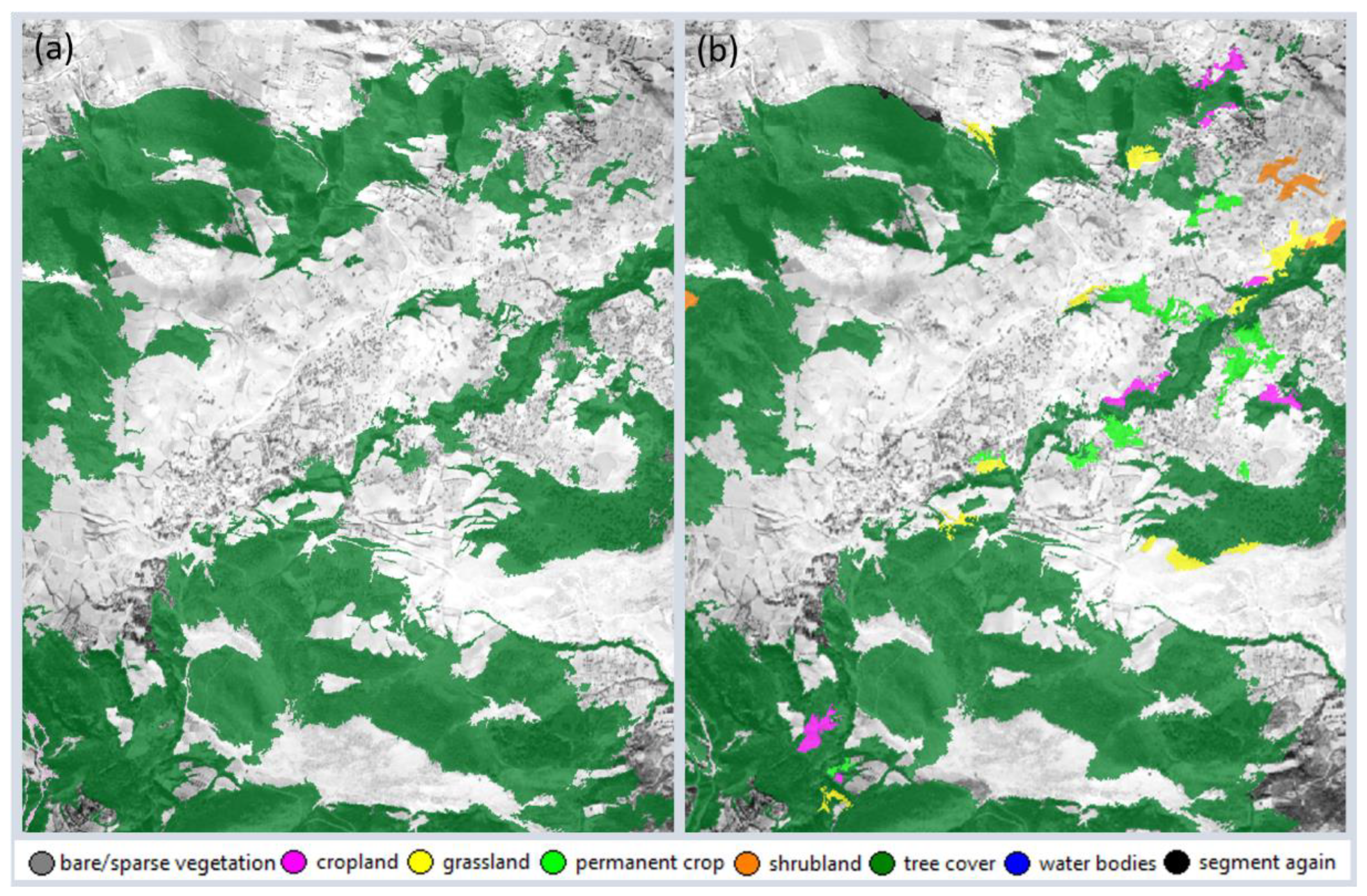
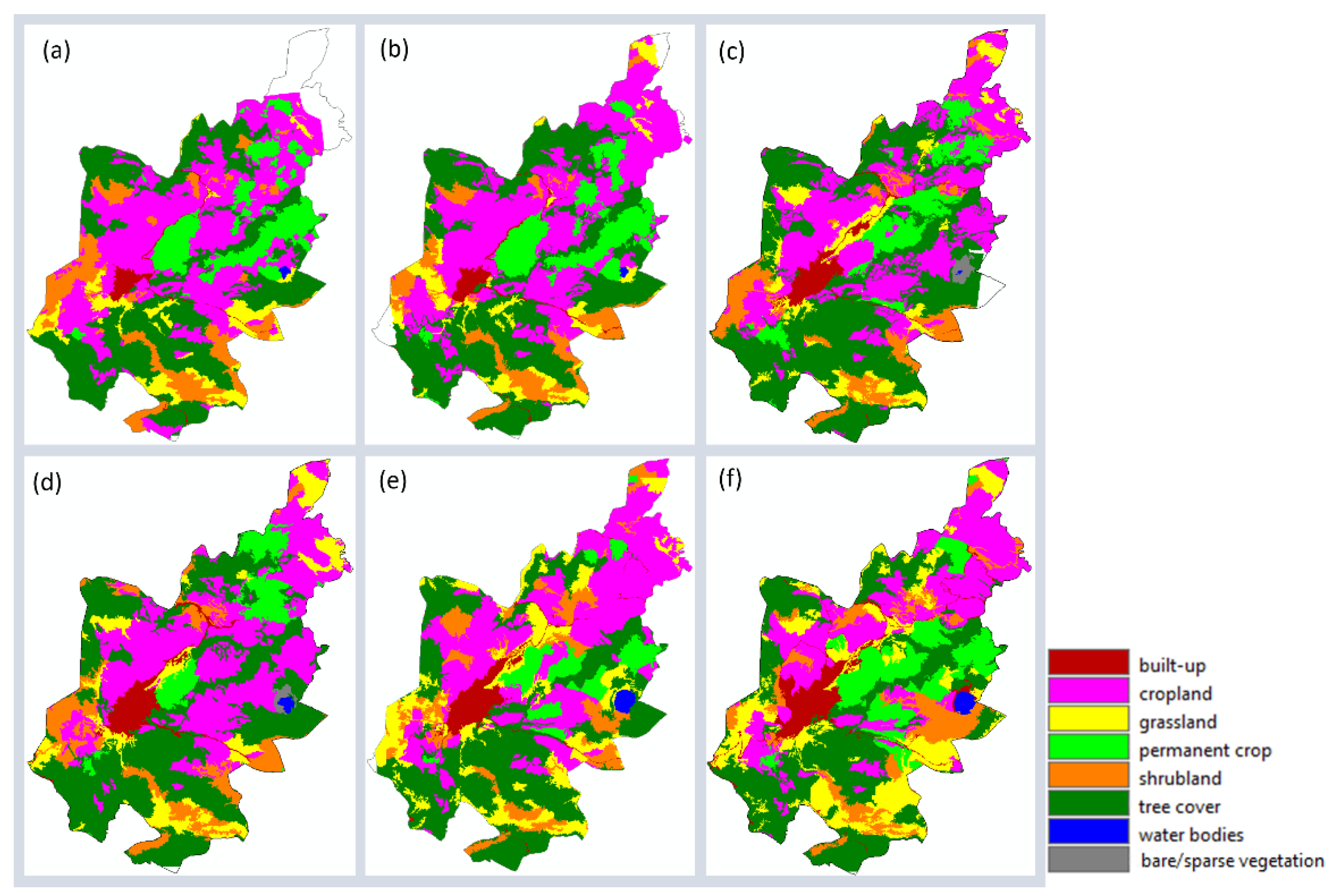
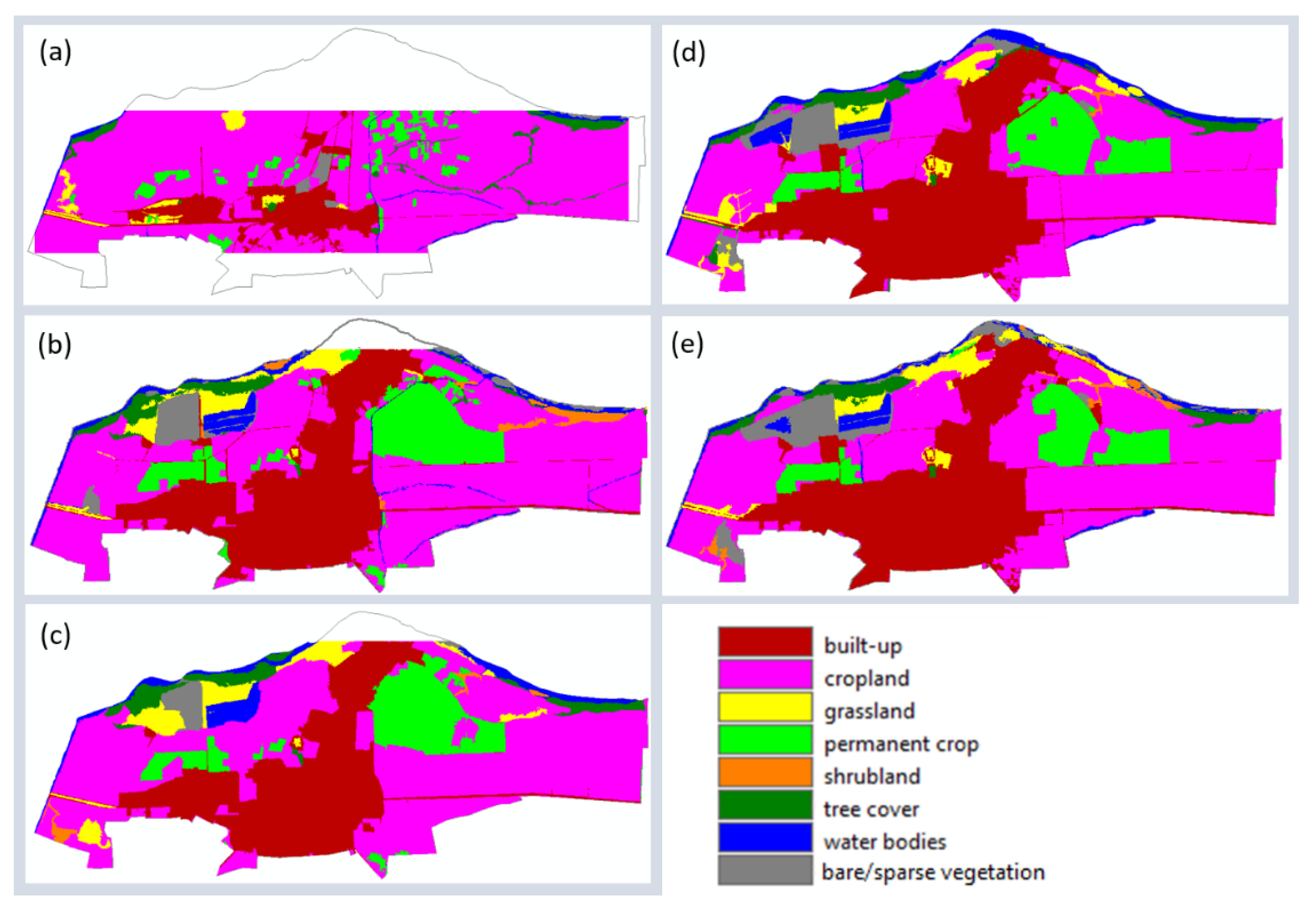
3. Results for Each Date—Visual Interpretation and Statistical Analysis

Figure 17 presents the LULC map of the Ruen site in 1945, 1952, 1965, 1968, 1975, and 1980, the classification results of the aerial photographs (1945–1952–1965–1975), Corona satellite image (1968), and Hexagon imagery (1980). Table 9 presents the statistical analysis of the land cover classes in each of the land cover maps.
Drastic rural depopulation (from 716 in 1946, to 211 in 1985; see Table 1) resulted in a decrease of 1/3 in cropland for Ruen in the last decade under investigation. This development is in accordance with expectations of rural depopulation’s retarded impact on agricultural land abandonment. Figure 18 presents the LULC map of the Stamboliyski site in 1952, 1965, 1968, 1975, and 1980, the classification results of the aerial photographs (1952–1965–1975), Corona satellite image (1968), and Hexagon imagery (1980). Table 10 presents the statistical analysis of the land cover classes in each of the land cover maps.
Fast early urbanization of Stamboliyski (from 3,224 in 1946, to 7,866 in 1956, and 12,804 in 1965; see Table 1) and then leveling of population growth (from 13,313 in 1975, to 13,449 in 1985; see Table 1) can be seen reflected in a rapid and then gradual increase in the built-up area. The mirror image of this dynamic can be observed in the fast fall but then leveling of cropland.

4. Discussion

Accurate identification of the spatio-temporal distribution of LULC classes is essential to understanding past human activities and their impact on the environment, such as agricultural land abandonment, urbanization, and deforestation. Although there are complicated algorithms to process recent high-resolution aerial photographs and satellite images, this is a challenging task for historical photographs and satellite platforms, such as Corona and Hexagon. The problem is mainly due to their limited spectral and radiometric resolutions and the availability of various geometric distortions. With the recent public availability of Hexagon images, reliable methodologies for the geometric correction and classification of these images and integrated usage of these images with another historical geospatial dataset became important. Although there are several studies with Corona KH-4 images, studies with Hexagon images are fairly limited [43,48,87,88]. First studies with Hexagon KH-9 images were generally conducted for glacier monitoring, archaeology, and digital surface model generation, similar to Corona images [48,50,51,52,54,57,89,90,91]. The number of LULC mapping studies with Key Hole satellites is minimal, and a few studies were conducted with Corona images [41,43]. Utilizing visual interpretation methods, Fekete [45] used all Key Hole satellite series, including KH-9 Hexagon, to determine natural hazard risk and urban growth. Rashid and Aneaus used high-resolution declassified satellite data from 1965 (from Corona mission) and 1980 (Hexagon mission) to quantify land system changes. They employed on-screen digitization, with cognitive inputs from analysts [92]. Prokop utilized a Corona image from October 1965 to detect long-term land-use changes and they applied a visual interpretation technique for the LULC mapping [93]. Our study is unique in terms of the proposed methodology and the usage of Hexagon data in conjuction with other historical geospatial data for the LULC mapping perspective. We applied a feasible geometric correction approach by implementing rubber sheeting and collecting reference points from the Google Earth system that can be transferred to any other geographic region if similar datasets are available. Most of the studies in the literature use manual vectorization techniques, which are time-consuming and subjective. We propose an iterative GeOBIA approach to accurately generate multi-temporal LULC maps from multi-modal data, which researchers can use for various purposes in the case of similar remotely sensed data. Specifically, scale parameters specific to different land categories could be applied to various geographical areas in the case of using similar geospatial data sources. Historical census data is also an essential information source to understand and interpret historical LULC changes.
Implementing the ESA WoldCover project’s LULC classes with a modification in tree classes to determine permanent agriculture classes is also unique to our study, which is essential to monitor agricultural changes apart from forests. After revising current ESA WorldCover data for tree cover classes and quality controlling its accuracy, a comparison could also be made to detect LULC changes from the 1940s to today, which will be considered in our future work. However, it is important to emphasize that ESA WorldCover product resolution is 10 m, which is lower than our very-high resolution historical geospatial data; therefore, generalization might be needed, resulting in the loss of some spatial details. Another alternative is to use VHR satellite or UAV images to find the long-term changes from the past to today, something that we will consider in our future work to find up-to-date VHR data.

5. Conclusions

Agricultural land abandonment is a massive threat to the population geography of Bulgaria, which has one of the fastest shrinking populations on a national scale worldwide. Combined with an ongoing rural depopulation, agricultural land abandonment will probably cause a rural population collapse in Bulgaria in the coming decades. Therefore, it is crucial to understand the timing and magnitude of these decisive demographic and economic changes. Our study roughly examines the first three decades of communist rule in Bulgaria, during which drastic social engineering practices, including radical collectivizations in the agricultural sector, have occurred. In both of our chosen locations, we can see a decrease in cropland in the period. This finding is striking at first glance, since we opted for Ruen as a representative example of stark rural depopulation and Stamboliyski for urban development. The fact that we observe a fall in Ruen and stagnancy in Stamboliyski, in the areas used for agricultural production in the period, hints at a systematic issue, most probably politically caused, and long in the making of agricultural land abandonment.

Author Contributions

Conceptualization, M.E.K. and E.S.; methodology, M.E.K. and E.S.; software, P.E.O.; validation, E.S. and P.E.O.; formal analysis, P.E.O. and E.S.; investigation, M.E.K., E.S. and P.E.O.; resources, M.E.K. and E.S.; data curation, M.E.K. and P.E.O.; writing—original draft preparation, M.E.K., P.E.O. and E.S.; writing—review and editing, M.E.K., E.S. and P.E.O.; visualization, P.E.O.; supervision, M.E.K. and E.S.; project administration, M.E.K.; funding acquisition, M.E.K. All authors have read and agreed to the published version of the manuscript.

Funding

This work was supported by the European Research Council (ERC) project: “Industrialisation and Urban Growth from the mid-nineteenth century Ottoman Empire to Contemporary Turkey in a Comparative Perspective, 1850–2000” under the European Union’s Horizon 2020 research and innovation program Grant Agreement No. 679097, acronym UrbanOccupationsOETR. M. Erdem Kabadayı is the principal investigator of UrbanOccupationsOETR.

Data Availability Statement

Not applicable.

Conflicts of Interest

The authors declare no conflict of interest.

References

  1. Subedi, Y.R.; Kristiansen, P.; Cacho, O. Drivers and Consequences of Agricultural Land Abandonment and Its Reutilisation Pathways: A Systematic Review. Environ. Dev. 2022, 42, 100681. [Google Scholar] [CrossRef]
  2. Perpina Castillo, C.; Kavalov, B.; Diogo, V.; Jacobs-Crisioni, C.; Batista e Silva, F.; Lavalle, C. Agricultural Land Abandonment in the EU within 2015–2030; Joint Research Centre (Seville Site): Seville, Spain, 2018. [Google Scholar]
  3. Emmerson, M.; Morales, M.B.; Oñate, J.J.; Batáry, P.; Berendse, F.; Liira, J.; Aavik, T.; Guerrero, I.; Bommarco, R.; Eggers, S.; et al. Chapter Two—How Agricultural Intensification Affects Biodiversity and Ecosystem Services. In Advances in Ecological Research; Dumbrell, A.J., Kordas, R.L., Woodward, G., Eds.; Large-Scale Ecology: Model Systems to Global Perspectives; Academic Press: New York, NY, USA, 2016; Volume 55, pp. 43–97. [Google Scholar]
  4. Ustaoglu, E.; Collier, M.J. Farmland Abandonment in Europe: An Overview of Drivers, Consequences, and Assessment of the Sustainability Implications. Environ. Rev. 2018, 26, 396–416. [Google Scholar] [CrossRef]
  5. Levers, C.; Schneider, M.; Prishchepov, A.V.; Estel, S.; Kuemmerle, T. Spatial Variation in Determinants of Agricultural Land Abandonment in Europe. Sci. Total Environ. 2018, 644, 95–111. [Google Scholar] [CrossRef] [PubMed]
  6. Lasanta, T.; Arnáez, J.; Pascual, N.; Ruiz-Flaño, P.; Errea, M.P.; Lana-Renault, N. Space–Time Process and Drivers of Land Abandonment in Europe. CATENA 2017, 149, 810–823. [Google Scholar] [CrossRef]
  7. Lavalle, C.; Silva, F.B.E.; Baranzelli, C.; Jacobs-Crisioni, C.; Kompil, M.; Perpiña Castillo, C.; Vizcaino, P.; Ribeiro Barranco, R.; Vandecasteele, I.; Kavalov, B.; et al. The LUISA Territorial Modelling Platform and Urban Data Platform: An EU-Wide Holistic Approach. In Territorial Impact Assessment; Medeiros, E., Ed.; Advances in Spatial Science; Springer International Publishing: Cham, Switzerland, 2020; pp. 177–194. ISBN 978-3-030-54502-4. [Google Scholar]
  8. Perpiña Castillo, C.; Jacobs-Crisioni, C.; Diogo, V.; Lavalle, C. Modelling Agricultural Land Abandonment in a Fine Spatial Resolution Multi-Level Land-Use Model: An Application for the EU. Environ. Model. Softw. 2021, 136, 104946. [Google Scholar] [CrossRef]
  9. Mallinis, G.; Emmanoloudis, D.; Giannakopoulos, V.; Maris, F.; Koutsias, N. Mapping and Interpreting Historical Land Cover/Land Use Changes in a Natura 2000 Site Using Earth Observational Data: The Case of Nestos Delta, Greece. Appl. Geogr. 2011, 31, 312–320. [Google Scholar] [CrossRef]
  10. Sheeren, D.; Ladet, S.; Ribière, O.; Raynaud, B.; Paegelow, M.; Houet, T. Assessing Land Cover Changes in the French Pyrenees since the 1940s: A Semi-Automatic GEOBIA Approach Using Aerial Photographs. In Proceedings of the Multidisciplinary Research on Geographical Information in Europe and Beyond, Avignon, France, 24–27 April 2012; p. 3. [Google Scholar]
  11. Xystrakis, F.; Psarras, T.; Koutsias, N. A Process-Based Land Use/Land Cover Change Assessment on a Mountainous Area of Greece during 1945–2009: Signs of Socio-Economic Drivers. Sci. Total Environ. 2017, 587–588, 360–370. [Google Scholar] [CrossRef]
  12. Janus, J.; Bożek, P.; Taszakowski, J.; Doroż, A. Decaying Villages in the Centre of Europe with No Population Decline: Long-Term Analysis Using Historical Aerial Images and Remote Sensing Data. Habitat Int. 2022, 121, 102520. [Google Scholar] [CrossRef]
  13. Cousins, S.A.O. Analysis of Land-Cover Transitions Based on 17th and 18th Century Cadastral Maps and Aerial Photographs. Landsc. Ecol. 2001, 16, 41–54. [Google Scholar] [CrossRef]
  14. Sobala, M. Landscape Effects of Conflicts in Space Management. A Historical Approach Based on the Silesian and Żywiec Beskids (West Carpathians, Poland). Environ. Socio-Econ. Stud. 2016, 4, 51–60. [Google Scholar] [CrossRef]
  15. Sobala, M.; Rahmonov, O.; Myga-Piatek, U. Historical and Contemporary Forest Ecosystem Changes in the Beskid Mountains (Southern Poland) between 1848 and 2014. iFor. Biogeosci. For. 2017, 10, 939–947. [Google Scholar] [CrossRef] [Green Version]
  16. Solarski, M.; Krzysztofik, R. Is the Naturalization of the Townscape a Condition of De-Industrialization? An Example of Bytom in Southern Poland. Land 2021, 10, 838. [Google Scholar] [CrossRef]
  17. Ettehadi Osgouei, P.; Sertel, E.; Kabadayı, M.E. Integrated Usage of Historical Geospatial Data and Modern Satellite Images Reveal Long-Term Land Use/Cover Changes in Bursa/Turkey, 1858–2020. Sci. Rep. 2022, 12, 9077. [Google Scholar] [CrossRef]
  18. Rodríguez-Soler, R.; Uribe-Toril, J.; De Pablo Valenciano, J. Worldwide Trends in the Scientific Production on Rural Depopulation, a Bibliometric Analysis Using Bibliometrix R-Tool. Land Use Policy 2020, 97, 104787. [Google Scholar] [CrossRef]
  19. Sluiter, R.; de Jong, S.M. Spatial Patterns of Mediterranean Land Abandonment and Related Land Cover Transitions. Landsc. Ecol. 2007, 22, 559–576. [Google Scholar] [CrossRef]
  20. Bruno, D.; Sorando, R.; Álvarez-Farizo, B.; Castellano, C.; Céspedes, V.; Gallardo, B.; Jiménez, J.J.; López, M.V.; López-Flores, R.; Moret-Fernández, D.; et al. Depopulation Impacts on Ecosystem Services in Mediterranean Rural Areas. Ecosyst. Serv. 2021, 52, 101369. [Google Scholar] [CrossRef]
  21. Quaranta, G.; Salvia, R.; Salvati, L.; Paola, V.D.; Coluzzi, R.; Imbrenda, V.; Simoniello, T. Long-Term Impacts of Grazing Management on Land Degradation in a Rural Community of Southern Italy: Depopulation Matters. Land Degrad. Dev. 2020, 31, 2379–2394. [Google Scholar] [CrossRef]
  22. Stratoulias, D.; Kabadayı, M.E. Feature and Information Extraction for Regions of Southeast Europe from Corona Satellite Images Acquired in 1968. In Proceedings of the Eighth International Conference on Remote Sensing and Geoinformation of the Environment (RSCy2020); International Society for Optics and Photonics, Paphos, Cyprus, 26 August 2020; Volume 11524. [Google Scholar]
  23. Stratoulias, D.; Kabadayı, M.E. Land Cover Feature Extraction from Corona Spy Satellite Images During the Cold WAR—1968. In Proceedings of the IGARSS 2020—2020 IEEE International Geoscience and Remote Sensing Symposium, Waikoloa, HI, USA, 26 September–2 October 2020; pp. 6069–6072. [Google Scholar]
  24. Stratoulias, D.; Grekousis, G. Information Extraction and Population Estimates of Settlements from Historic Corona Satellite Imagery in the 1960s. Sensors 2021, 21, 2423. [Google Scholar] [CrossRef]
  25. Gutman, G.; Radeloff, V. Land-Cover and Land-Use Changes in Eastern Europe after the Collapse of the Soviet Union in 1991; Springer International Publishing: Cham, Switzerland, 2017; ISBN 978-3-319-42636-5. [Google Scholar]
  26. Marinova, T.; Nenovsky, N. Cooperative Agricultural Farms in Bulgaria during Communism (1944–1989): An Institutional Reconstruction. Rom. Econ. J. 2019, XXII, 40–73. [Google Scholar]
  27. Pangelova, B.; Rogan, J. Land Cover and Land Use Change Detection and Analyses in Plovdiv, Bulgaria, Between 1986 and 2000. In Proceedings of the ASPRS 2006 Annual Conference, Reno, Nevada, 1–5 May 2006. [Google Scholar]
  28. Feranec, J.; Kopecka, M.; Vatseva, R.; Stoimenov, A.; Otahel, J.; Betak, J.; Husar, K. Landscape Change Analysis and Assessment (Case Studies in Slovakia and Bulgaria). Open Geosci. 2009, 1, 106–119. [Google Scholar] [CrossRef]
  29. Kitev, A. Impact of Settlements on the Landscapes of Slavyanka Mountain (South-Western Bulgaria). J. Settl. Spat. Plan. 2014, 3, 65–69. [Google Scholar]
  30. Avetisyan, D.; Velizarova, E.; Nedkov, R.; Borisova, D. Assessment and Mapping of the Current State of the Landscapes/Ecosystems in Haskovo Region (Southeastern Bulgaria) in Relation to Ecosystem Services Using Remote Sensing and GIS. In Proceedings of the Sixth International Conference on Remote Sensing and Geoinformation of the Environment (RSCy2018), Paphos, Cyprus, 6 August 2018; Volume 10773, pp. 555–563. [Google Scholar]
  31. Eftimoski, M.; Ross, S.A.; Sobotkova, A. The Impact of Land Use and Depopulation on Burial Mounds in the Kazanlak Valley, Bulgaria: An Ordered Logit Predictive Model. J. Cult. Herit. 2017, 23, 1–10. [Google Scholar] [CrossRef]
  32. Mladenov, C.; Dimitrov, E.; Kazakov, B. Demographical Development of Bulgaria during the Transitional Period. J. Mediterr. Geogr. 2008, 110, 117–123. [Google Scholar] [CrossRef]
  33. Ilieva, M.; Mladenov, C. Changes in the Rural Areas in Bulgaria: Processes and Prospects. Geogr. Pol. 2003, 76, 97–110. [Google Scholar]
  34. Mladenov, C.; Ilieva, M. The Depopulation of the Bulgarian Villages. Bull. Geography. Socio-Econ. Ser. 2012, 17, 99–107. [Google Scholar] [CrossRef] [Green Version]
  35. Koulov, B.; Boyadjiev, V.; Ravnachka, A. The Demographyc Draining of Bulgaria’s Rural Area: A GIS-Aided Geospatial Analysis (1992–2017). In Three Decades of Transformation in the East-Central European Countryside; Bański, J., Ed.; Springer International Publishing: Cham, Switzerland, 2019; pp. 239–260. ISBN 978-3-030-21237-7. [Google Scholar]
  36. Dashora, A.; Lohani, B.; Malik, J.N. A Repository of Earth Resource Information—CORONA Satellite Programme. Curr. Sci. 2007, 92, 926–932. [Google Scholar]
  37. Coskun Hepcan, C. Quantifying Landscape Pattern and Connectivity in a Mediterranean Coastal Settlement: The Case of the Urla District, Turkey. Environ. Monit. Assess. 2013, 185, 143–155. [Google Scholar] [CrossRef]
  38. Mihai, B.; Nistor, C.; Toma, L.; Săvulescu, I. High Resolution Landscape Change Analysis with CORONA KH-4B Imagery. A Case Study from Iron Gates Reservoir Area. Procedia Environ. Sci. 2016, 32, 200–210. [Google Scholar] [CrossRef] [Green Version]
  39. Saleem, A. Using CORONA and Landsat Data for Evaluating and Mapping Long-Term LULC Changes in Iraqi Kurdistan. Ph.D. Thesis, Curtin University, Perth, Australia, 2017. [Google Scholar]
  40. Shahtahmassebi, A.R.; Lin, Y.; Lin, L.; Atkinson, P.M.; Moore, N.; Wang, K.; He, S.; Huang, L.; Wu, J.; Shen, Z.; et al. Reconstructing Historical Land Cover Type and Complexity by Synergistic Use of Landsat Multispectral Scanner and CORONA. Remote Sens. 2017, 9, 682. [Google Scholar] [CrossRef] [Green Version]
  41. Nita, M.D.; Munteanu, C.; Gutman, G.; Abrudan, I.V.; Radeloff, V.C. Widespread Forest Cutting in the Aftermath of World War II Captured by Broad-Scale Historical Corona Spy Satellite Photography. Remote Sens. Environ. 2018, 204, 322–332. [Google Scholar] [CrossRef]
  42. Saleem, A.; Corner, R.; Awange, J. On the Possibility of Using CORONA and Landsat Data for Evaluating and Mapping Long-Term LULC: Case Study of Iraqi Kurdistan. Appl. Geogr. 2018, 90, 145–154. [Google Scholar] [CrossRef]
  43. Gurjar, S.K.; Tare, V. Estimating Long-Term LULC Changes in an Agriculture-Dominated Basin Using CORONA (1970) and LISS IV (2013–14) Satellite Images: A Case Study of Ramganga River, India. Environ. Monit. Assess. 2019, 191, 217. [Google Scholar] [CrossRef]
  44. Akın, A.; Erdoğan, M.A. Analysing Temporal and Spatial Urban Sprawl Change of Bursa City Using Landscape Metrics and Remote Sensing. Model. Earth Syst. Environ. 2020, 6, 1331–1343. [Google Scholar] [CrossRef]
  45. Fekete, A. CORONA High-Resolution Satellite and Aerial Imagery for Change Detection Assessment of Natural Hazard Risk and Urban Growth in El Alto/La Paz in Bolivia, Santiago de Chile, Yungay in Peru, Qazvin in Iran, and Mount St. Helens in the USA. Remote Sens. 2020, 12, 3246. [Google Scholar] [CrossRef]
  46. Rendenieks, Z.; Nita, M.D.; Nikodemus, O.; Radeloff, V.C. Half a Century of Forest Cover Change along the Latvian-Russian Border Captured by Object-Based Image Analysis of Corona and Landsat TM/OLI Data. Remote Sens. Environ. 2020, 249, 112010. [Google Scholar] [CrossRef]
  47. Deshpande, P.; Belwalkar, A.; Dikshit, O.; Tripathi, S. Historical Land Cover Classification from CORONA Imagery Using Convolutional Neural Networks and Geometric Moments. Int. J. Remote Sens. 2021, 42, 5144–5171. [Google Scholar] [CrossRef]
  48. Krina, A.; Xystrakis, F.; Karantininis, K.; Koutsias, N. Monitoring and Projecting Land Use/Land Cover Changes of Eleven Large Deltaic Areas in Greece from 1945 Onwards. Remote Sens. 2020, 12, 1241. [Google Scholar] [CrossRef] [Green Version]
  49. Pressel, P. Meeting the Challenge: The Hexagon KH-9 Reconnaissance Satellite; Allen, N., Ed.; American Institute of Aeronautics and Astronautics (AIAA): Reston, VA, USA, 2013; ISBN 978-1-62410-204-2. [Google Scholar]
  50. Pieczonka, T.; Bolch, T.; Junfeng, W.; Shiyin, L. Heterogeneous Mass Loss of Glaciers in the Aksu-Tarim Catchment (Central Tien Shan) Revealed by 1976 KH-9 Hexagon and 2009 SPOT-5 Stereo Imagery. Remote Sens. Environ. 2013, 130, 233–244. [Google Scholar] [CrossRef] [Green Version]
  51. Fowler, M.J.F. The Archaeological Potential of Declassified HEXAGON KH-9 Panoramic Camera Satellite Photographs. AARG News 2016, 53, 30–36. [Google Scholar]
  52. Fowler, M.J.F. Declassified Intelligence Satellite Photographs. In Archaeology from Historical Aerial and Satellite Archives; Hanson, W.S., Oltean, I.A., Eds.; Springer: New York, NY, USA, 2013; pp. 47–66. ISBN 978-1-4614-4505-0. [Google Scholar]
  53. Hammer, E.; FitzPatrick, M.; Ur, J. Succeeding CORONA: Declassified HEXAGON Intelligence Imagery for Archaeological and Historical Research. Antiquity 2022, 96, 679–695. [Google Scholar] [CrossRef]
  54. Holzer, N.; Vijay, S.; Yao, T.; Xu, B.; Buchroithner, M.; Bolch, T. Four Decades of Glacier Variations at Muztagh Ata (Eastern Pamir): A Multi-Sensor Study Including Hexagon KH-9 and Pléiades Data. Cryosphere 2015, 9, 2071–2088. [Google Scholar] [CrossRef] [Green Version]
  55. Maurer, J.M.; Rupper, S.B.; Schaefer, J.M. Quantifying Ice Loss in the Eastern Himalayas since 1974 Using Declassified Spy Satellite Imagery. Cryosphere 2016, 10, 2203–2215. [Google Scholar] [CrossRef] [Green Version]
  56. Pieczonka, T.; Bolch, T. Region-Wide Glacier Mass Budgets and Area Changes for the Central Tien Shan between ~1975 and 1999 Using Hexagon KH-9 Imagery. Glob. Planet. Chang. 2015, 128, 1–13. [Google Scholar] [CrossRef]
  57. Lamsal, D.; Fujita, K.; Sakai, A. Surface Lowering of the Debris-Covered Area of Kanchenjunga Glacier in the Eastern Nepal Himalaya since 1975, as Revealed by Hexagon KH-9 and ALOS Satellite Observations. Cryosphere 2017, 11, 2815–2827. [Google Scholar] [CrossRef] [Green Version]
  58. Zhou, Y.; Li, Z.; Li, J.; Zhao, R.; Ding, X. Glacier Mass Balance in the Qinghai–Tibet Plateau and Its Surroundings from the Mid-1970s to 2000 Based on Hexagon KH-9 and SRTM DEMs. Remote Sens. Environ. 2018, 210, 96–112. [Google Scholar] [CrossRef]
  59. Bolch, T.; Yao, T.; Bhattacharya, A.; Hu, Y.; King, O.; Liu, L.; Pronk, J.B.; Rastner, P.; Zhang, G. Earth Observation to Investigate Occurrence, Characteristics and Changes of Glaciers, Glacial Lakes and Rock Glaciers in the Poiqu River Basin (Central Himalaya). Remote Sens. 2022, 14, 1927. [Google Scholar] [CrossRef]
  60. Surazakov, A.; Aizen, V. Positional Accuracy Evaluation of Declassified Hexagon KH-9 Mapping Camera Imagery. Photogramm. Eng. Remote Sens. 2010, 76, 603–608. [Google Scholar] [CrossRef] [Green Version]
  61. Maurer, J.; Rupper, S. Tapping into the Hexagon Spy Imagery Database: A New Automated Pipeline for Geomorphic Change Detection. ISPRS J. Photogramm. Remote Sens. 2015, 108, 113–127. [Google Scholar] [CrossRef]
  62. Dehecq, A.; Gardner, A.S.; Alexandrov, O.; McMichael, S.; Hugonnet, R.; Shean, D.; Marty, M. Automated Processing of Declassified KH-9 Hexagon Satellite Images for Global Elevation Change Analysis Since the 1970s. Front. Earth Sci. 2020, 8, 566802. [Google Scholar] [CrossRef]
  63. Drummond, M.A.; Stier, M.P.; Diffendorfer, J.J.E. Historical Land Use and Land Cover for Assessing the Northern Colorado Front Range Urban Landscape. J. Maps 2019, 15, 89–93. [Google Scholar] [CrossRef]
  64. Peña-Angulo, D.; Khorchani, M.; Errea, P.; Lasanta, T.; Martínez-Arnáiz, M.; Nadal-Romero, E. Factors Explaining the Diversity of Land Cover in Abandoned Fields in a Mediterranean Mountain Area. CATENA 2019, 181, 104064. [Google Scholar] [CrossRef]
  65. Gerard, F.; Petit, S.; Smith, G.; Thomson, A.; Brown, N.; Manchester, S.; Wadsworth, R.; Bugar, G.; Halada, L.; Bezák, P.; et al. Land Cover Change in Europe between 1950 and 2000 Determined Employing Aerial Photography. Prog. Phys. Geogr. Earth Environ. 2010, 34, 183–205. [Google Scholar] [CrossRef] [Green Version]
  66. Ruelland, D.; Tribotte, A.; Puech, C.; Dieulin, C. Comparison of Methods for LUCC Monitoring over 50 Years from Aerial Photographs and Satellite Images in a Sahelian Catchment. Int. J. Remote Sens. 2011, 32, 1747–1777. [Google Scholar] [CrossRef]
  67. Liu, D.; Toman, E.; Fuller, Z.; Chen, G.; Londo, A.; Zhang, X.; Zhao, K. Integration of Historical Map and Aerial Imagery to Characterize Long-Term Land-Use Change and Landscape Dynamics: An Object-Based Analysis via Random Forests. Ecol. Indic. 2018, 95, 595–605. [Google Scholar] [CrossRef]
  68. Vogels, M.F.A.; de Jong, S.M.; Sterk, G.; Addink, E.A. Agricultural Cropland Mapping Using Black-and-White Aerial Photography, Object-Based Image Analysis and Random Forests. Int. J. Appl. Earth Obs. Geoinf. 2017, 54, 114–123. [Google Scholar] [CrossRef]
  69. United Nations Department of Economic and Social Affairs. Population Division. World Population Prospects 2022: Summary of Results; United Nations Department of Economic and Social Affairs: New York, NY, USA, 2022. [Google Scholar]
  70. Mihaylov, V.T. Ethnic and Regional Aspects of the Demographic Crisis in Bulgaria. Reg. Res. Russ. 2021, 11, 254–262. [Google Scholar] [CrossRef]
  71. Traykov, T.; Naydenov, K. Demographic Situation in Rural Areas of Republic of Bulgaria in 21 Century. In Proceedings of the 1st International Scientific Conference Geobalcanica, Skopje, Republic of Macedonia, 5–7 June 2015; pp. 201–208. [Google Scholar]
  72. National Register of Populated Places, National Statistical Institute of the Republic of Bulgaria. Available online: https://www.nsi.bg/nrnm/index.php?f=9&ezik=en (accessed on 1 October 2022).
  73. Chen, G.; Weng, Q.; Hay, G.J.; He, Y. Geographic Object-Based Image Analysis (GEOBIA): Emerging Trends and Future Opportunities. GISci. Remote Sens. 2018, 55, 159–182. [Google Scholar] [CrossRef]
  74. Cao, J.; Fu, J.; Yuan, X.; Gong, J. Nonlinear Bias Compensation of ZiYuan-3 Satellite Imagery with Cubic Splines. ISPRS J. Photogramm. Remote Sens. 2017, 133, 174–185. [Google Scholar] [CrossRef]
  75. Topaloğlu, R.H.; Aksu, G.A.; Ghale, Y.A.G.; Sertel, E. High-Resolution Land Use and Land Cover Change Analysis Using GEOBIA and Landscape Metrics: A Case of Istanbul, Turkey. Geocarto Int. 2021, 36, 1–27. [Google Scholar] [CrossRef]
  76. Janata, T.; Cajthaml, J. Georeferencing of Multi-Sheet Maps Based on Least Squares with Constraints—First Military Mapping Survey Maps in the Area of Czechia. Appl. Sci. 2021, 11, 299. [Google Scholar] [CrossRef]
  77. Rocco, I.; Arandjelovic, R.; Sivic, J. Convolutional Neural Network Architecture for Geometric Matching. IEEE Trans. Pattern Anal. Mach. Intell. 2019, 41, 2553–2567. [Google Scholar] [CrossRef] [Green Version]
  78. Zitová, B.; Flusser, J. Image Registration Methods: A Survey. Image Vis. Comput. 2003, 21, 977–1000. [Google Scholar] [CrossRef] [Green Version]
  79. Ye, S.; Pontius, R.G.; Rakshit, R. A Review of Accuracy Assessment for Object-Based Image Analysis: From per-Pixel to per-Polygon Approaches. ISPRS J. Photogramm. Remote Sens. 2018, 141, 137–147. [Google Scholar] [CrossRef]
  80. Myint, S.W.; Gober, P.; Brazel, A.; Grossman-Clarke, S.; Weng, Q. Per-Pixel vs. Object-Based Classification of Urban Land Cover Extraction Using High Spatial Resolution Imagery. Remote Sens. Environ. 2011, 115, 1145–1161. [Google Scholar] [CrossRef]
  81. Baatz, M.; Schape, A. Multiresolution Segmentation: An Optimization Approach for High Quality Multi-Scale Image Segmentation. In XII Angewandte Geographische Informationsverarbeitung; Wichmann-Verlag: Heidelberg, Germany, 2000; pp. 12–23. [Google Scholar]
  82. Darwish, A.; Leukert, K.; Reinhardt, W. Image Segmentation for the Purpose of Object-Based Classification. In Proceedings of the IEEE International Geoscience and Remote Sensing Symposium, Toulouse, France, 21–25 July 2003. [Google Scholar]
  83. Blaschke, T. Object Based Image Analysis for Remote Sensing. ISPRS J. Photogramm. Remote Sens. 2010, 65, 2–16. [Google Scholar] [CrossRef]
  84. Tian, J.; Chen, D.-M. Optimization in Multi-scale Segmentation of High-resolution Satellite Images for Artificial Feature Recognition. Int. J. Remote Sens. 2007, 28, 4625–4644. [Google Scholar] [CrossRef]
  85. Lucas, R.; Rowlands, A.; Brown, A.; Keyworth, S.; Bunting, P. Rule-Based Classification of Multi-Temporal Satellite Imagery for Habitat and Agricultural Land Cover Mapping. ISPRS J. Photogramm. Remote Sens. 2007, 62, 165–185. [Google Scholar] [CrossRef]
  86. Bauer, T.; Strauss, P. A Rule-Based Image Analysis Approach for Calculating Residues and Vegetation Cover under Field Conditions. Catena 2014, 113, 363–369. [Google Scholar] [CrossRef]
  87. Goossens, R.; De Wulf, A.; Bourgeois, J.; Gheyle, W.; Willems, T. Satellite Imagery and Archaeology: The Example of CORONA in the Altai Mountains. J. Archaeol. Sci. 2006, 33, 745–755. [Google Scholar] [CrossRef]
  88. Beck, A.; Philip, G.; Abdulkarim, M.; Donoghue, D. Evaluation of Corona and Ikonos High Resolution Satellite Imagery for Archaeological Prospection in Western Syria. Antiquity 2007, 81, 161–175. [Google Scholar] [CrossRef] [Green Version]
  89. Goerlich, F.; Bolch, T.; Mukherjee, K.; Pieczonka, T. Glacier Mass Loss during the 1960s and 1970s in the Ak-Shirak Range (Kyrgyzstan) from Multiple Stereoscopic Corona and Hexagon Imagery. Remote Sens. 2017, 9, 275. [Google Scholar] [CrossRef] [Green Version]
  90. Altmaier, A.; Kany, C. Digital Surface Model Generation from CORONA Satellite Images. ISPRS J. Photogramm. Remote Sens. 2002, 56, 221–235. [Google Scholar] [CrossRef]
  91. Watanabe, N.; Nakamura, S.; Liu, B.; Wang, N. Utilization of Structure from Motion for Processing CORONA Satellite Images: Application to Mapping and Interpretation of Archaeological Features in Liangzhu Culture, China. Archaeol. Res. Asia 2017, 11, 38–50. [Google Scholar] [CrossRef]
  92. Rashid, I.; Aneaus, S. Landscape Transformation of an Urban Wetland in Kashmir Himalaya, India Using High-Resolution Remote Sensing Data, Geospatial Modeling, and Ground Observations over the Last 5 Decades (1965–2018). Environ. Monit. Assess. 2020, 192, 635. [Google Scholar] [CrossRef] [PubMed]
  93. Prokop, P. Remote Sensing of Severely Degraded Land: Detection of Long-Term Land-Use Changes Using High-Resolution Satellite Images on the Meghalaya Plateau, Northeast India. Remote Sens. Appl. Soc. Environ. 2020, 20, 100432. [Google Scholar] [CrossRef]
Figure 1. Location of Plovdiv district in Bulgaria and two populated regions as study sites in Plovdiv district (a) Bulgaria, (b) Plovdiv district, (c) Stamboliyski, and (d) Ruen.
Land 11 01855 g001
Figure 2. Footprints of selected Corona (blue and yellow) and Hexagon images (red and green) on Google Earth image. The areas shaded by cyan and pink show Stamboliyski and Ruen, respectively.
Land 11 01855 g002
Figure 3. (a) Distribution of GCPs on the 1975 aerial photo and examples of GCPs selection (red crosses) on (b) aerial photographs and their counterparts on (c) Google Earth, image indexed by colored boxes on the image (yellow vector shows the boundaries of the Ruen village).
Land 11 01855 g003
Figure 4. Examples of GCPs selection (red crosses) on (a,c,e) aerial photographs from 1952 and 1965, and their counterparts on (b,d,f) rectified 1975 Ruen aerial photograph.
Land 11 01855 g004
Figure 5. (a) 1945, (b,c) 1952, and (d,e) 1965 aerial photographs covering a portion of Ruen village, and mosaicked Ruen aerial photo of (f) 1952 and (g) 1965 (red vector shows the boundaries of the Ruen village).
Land 11 01855 g005
Figure 6. (a) Distribution of GCPs on two aerial photographs of Stamboliyski from 1975 and examples of GCPs selection (red crosses) on (b) aerial photographs and their counterparts on (c) Google Earth image.
Land 11 01855 g006
Figure 7. (a,b) Aerial photographs from 1975 covering a portion of Stamboliyski and (c) mosaicked 1975 aerial photographs. Red vector illustrates the boundaries of the Stamboliyski town.
Land 11 01855 g007
Figure 8. (ac) Aerial photographs from 1965 covering parts of Stamboliyski, and (d) mosaicked 1965 Stamboliyski aerial photograph. Red vector illustrates the boundaries of the Stamboliyski town.
Land 11 01855 g008
Figure 9. (ae) Aerial photographs from 1952 covering parts of Stamboliyski and (f) mosaicked 1952 Stamboliyski aerial photograph. Red vector illustrates the boundaries of the Stamboliyski town.
Land 11 01855 g009
Figure 10. Ruen village captured by (a) Corona image from 1968, (b,c) Hexagon images from 1975 and 1980, respectively (finer details of the region from Ruen village center are shown in the inset images highlighted by green boxes). Red vector illustrates the boundaries of the Stamboliyski town.
Land 11 01855 g010
Figure 11. Stamboliyski captured by (a) Corona image from 1968, (b,c) Hexagon images from 1975 and 1980, respectively (finer details of the region from Stamboliyski town center are shown in the inset images highlighted by green boxes).
Land 11 01855 g011
Figure 12. Comparisons of spatial resolutions of Ruen aerial photographs (a) 1945, (b) 1952, (c) 1965, and (d) 1975 and (e) 1968 Corona image, (f) 1975, and (g) 1980 Hexagon images.
Land 11 01855 g012
Figure 13. Examples representing the land cover classes.
Land 11 01855 g013
Figure 14. Segmented 1965 Ruen aerial photograph. Segments highlighted by red borders show the objects suitable for the “tree cover” class.
Land 11 01855 g014
Figure 15. Segmented 1965 Ruen aerial photograph. Segments highlighted by red borders show the objects resulting from small-scale segmentations.
Land 11 01855 g015
Figure 16. The 1952 Ruen aerial photograph (a) assigning the tree cover class to objects based on the 1965 Ruen land cover map (b) tree cover class objects after edition.
Land 11 01855 g016
Figure 17. Land cover maps of Ruen in: (a) 1945, (b) 1952, (c) 1965, (d) 1968, (e) 1975, (f) 1980.
Land 11 01855 g017
Figure 18. Land cover maps of Stamboliyski in: (a) 1952, (b) 1965, (c) 1968, (d)1975, (e)1980.
Land 11 01855 g018
Table 1. Total populations of Ruen and Stamboliyski. All the dates and figures are from national population censuses, except for 2020, which is based on national population estimates.
DateTotal Population of RuenTotal Population of Stamboliyski
19346911479
19467163224
19566067866
196540912,804
197532413,313
198521113,449
199217613,015
200117512,580
201115611,601
202026810,738
Table 2. Information about the satellite imageries used in the study, the number of Corona and Hexagon image subsets, and the used frame for covering the Ruen and Stamboliyski study sites.
ProjectMissionDateEntity IDTotal Frame Count Used Frame for RuenUsed Frame for Stamboliyski
CoronaKH-4B5 May 1968DS1103-1058DA0494-d
DS1103-1058DA0504d-
HexagonKH-912 July 1975D3C1210-200256A0377cd
HexagonKH-916 July 1980D3C1216-100235F05410ed
Table 3. The information about the aerial photographs used in the study.
DateNumber of Aerial Photographs of RuenNumber of Aerial Photographs of Stamboliyski
194510
195255
196533
197522
Table 4. Spatial resolutions of the Ruen and Stamboliyski geospatial dataset.
DateSpatial Resolution (m) of the Aerial Photographs of RuenSpatial Resolution (m) of the Aerial Photographs of StamboliyskiDateSpatial Resolution (m) of the Declassified Satellite Images of RuenSpatial Resolution (m) of the Declassified Satellite Images of Stamboliyski
19450.31-19682.712.93
19520.450.219751.060.93
19650.410.4319800.961.01
19750.550.57
Table 5. The overall accuracy and Kappa statistics of land cover maps of Ruen.
Data TypeDateOverall Accuracy (%)Kappa (%)
Aerial photographs194595.1794.21
195294.5793.63
196593.5792.59
Satellite images197593.8492.77
196891.4290.12
198093.0791.87
Table 6. The overall accuracy and Kappa statistics of land cover maps of Stamboliyski.
Data TypeDateOverall Accuracy (%)Kappa (%)
Aerial photographs195292.5991.35
196591.1189.81
197593.6092.59
Satellite images196894.1193.17
198091.1189.76
Table 7. Producer’s and user’s classification accuracies for the Ruen region.
Aerial PhotographsSatellite Images
194519521965197519681980
Land Cover ClassesPA (%)UA (%)PA (%)UA (%)PA (%)UA (%)PA (%)UA (%)PA (%)UA (%)PA (%)UA (%)
Built-up95.0010089.4710095.0010010010095.0010095.00100
Cropland10010010010095.0086.3690.0094.7495.0086.3610086.96
Grassland85.0010085.0094.4495.0090.4890.0085.7185.0077.2795.0090.48
Permanent Crop95.009510010085.0094.4495.0010080.0094.1290100
Shrubland90.0094.7490.0085.7185.0094.4485.0085.0085.0010080.0084.21
Tree Cover10085.7110086.9610090.9110095.2410090.9195.0095.00
Water Bodies100100100100100100100100100100100100
Bare/Sparse vegetation----100100--10090.91--
Table 8. Producer’s and user’s classification accuracies for the Stamboliyski region.
Aerial PhotographsSatellite Images
19521965197519681980
Land Cover ClassesPA (%)UA (%)PA (%)UA (%)PA (%)UA (%)PA (%)UA (%)PA (%)UA (%)
Built-up95.0090.4896.0010092.0092.0096.0010010092.59
Cropland95.0086.3696.0075.0010086.2110083.3310096.15
Grassland90.0010084.0091.3081.8294.7488.0010092.0079.31
Permanent Crop90.0094.7488.001009610084.0091.3096.00100
Shrubland--86.6786.6780.0010090.0010060.0075.00
Tree Cover95.0090.4890.0090.0010096.1510096.1584.0095.45
Water Bodies90.0010096.0010096.0010010092.5988.00100
Bare/Sparse vegetation93.3387.5090.0090.0090.0085.7190.0010090.0081.82
Table 9. Temporal evolution of the LULC classes in Ruen from 1945 to 1980 (in absolute numbers and percentages).
LC Class194519521965196819751980
Area (ha)%Area (ha)%Area (ha)%Area (ha)%Area (ha)%Area (ha)%
Bare/Sparse vegetation-0%-0%3.711%2.560%-0%-0%
Built-up8.392%10.322%18.463%21.634%22.444%34.016%
Cropland198.1336%208.3936%181.8431%189.9932%188.5832%148.7625%
Grassland36.937%39.537%44.048%51.369%82.0314%94.5216%
Permanent crop63.1311%63.8211%47.478%38.477%39.227%67.5312%
Shrubland61.6411%51.999%52.779%58.4810%58.7110%6511%
Tree cover184.5233%201.6135%232.6440%221.5338%190.9133%172.8930%
Water bodies0.790%0.620%0.150%1.540%3.471%3.261%
Table 10. Temporal evolution of the LULC classes in Stamboliyski from 1952 to 1980 (in absolute numbers and percentages).
LC Class19521965196819751980
Area (ha)%Area (ha)%Area (ha)%Area (ha)%Area (ha)%
Bare/Sparse vegetation11.191%43.643%21.782%59.794%76.195%
Built-up114.0911%362.7126%344.4125%423.2830%433.2531%
Cropland809.4377%655.7448%692.1750%614.4944%639.6545%
Grassland21.942%47.183%61.594%51.924%52.354%
Permanent crop49.85%157.9311%146.2111%133.5910%107.858%
Shrubland-0%19.081%8.371%2.380%14.041%
Tree cover28.763%39.163%48.354%48.643%36.543%
Water bodies13.91%48.053%50.864%71.945%46.183%
Publisher’s Note: MDPI stays neutral with regard to jurisdictional claims in published maps and institutional affiliations.

