High-Speed Railway Network Development, Inter-County Accessibility Improvements, and Regional Poverty Alleviation: Evidence from China

Abstract

The rapid expansion of the high-speed railway (HSR) network in China has significantly shortened the space–time distance between cities. China is striving to enter an anti-poverty era, which is increasing the importance of research on the poverty reduction effect created by upgrading transportation infrastructure, in particular, HSR development. Describing the characteristics of accessibility and the mechanisms by which that accessibility reduces poverty could provide the insights needed for determining suitable anti-poverty paths. By using data for 2341 counties and equivalents in China during 2007–2018, this study analyses the railway accessibility improvements and the poverty reduction effect created by HSR development. On average, HSR in China contributed to a significant increase in potential economic accessibility (317.8%) and a decrease in weighted average travel time (39.9%) for counties. Based on accessibility calculations, the Theil index was used to measure the disparity level of regional accessibility and regional poverty measured based on the income of rural residents. The results indicate that HSR leads to an increase in inequality in terms of travel time and potential economic accessibility at a national level. Pearson coefficients reveal a strong correlation between disparities in accessibility and in rural income among provinces. Furthermore, using the full sample, and sub-samples of poor and non-poor counties in China, the association between regional accessibility and poverty was examined by using two-way fixed effect models and spatial econometric models. The estimated results show that a 1% improvement in potential economic accessibility leads to an aggregate rural income improvement of 0.03–0.17%; the ratio of rural income to urban income increases by 0.04–0.12% and a larger effect is observed in poor counties. The weighted average travel time reduction also leads to improvement in rural income and reduction in the urban–rural income gap. The empirical results obtained by different robust test methods, including different sample groups, different estimated methods and accessibility indicators, are shown to be robust. These findings can help transportation departments formulate poverty-alleviation-oriented transportation planning and investment policies and inform future policies for countries planning to construct HSRs.

1. Introduction

In 2015, the United Nations released the 2030 Agenda for Sustainable Development, including 17 Sustainable Development Goals (SDGs), which were divided into 169 specific targets. The agenda stressed that integrated and systematic strategies should be adopted to achieve sustainable development within 15 years, and the three dimensions of sustainable development, economy, society and environment, should be balanced [1]. Eradication of poverty is the greatest global challenge and an indispensable requirement for sustainable development. Notably, poverty is closely related to social inequality. The first and tenth goals of the SDGs aim to “end poverty in all its forms everywhere” and “reduce inequality within and among countries”. In general, transportation is a significant factor in poverty reduction [2] and development of transportation can help to increase incomes for poverty-stricken people by increasing accessibility and economic efficiency [2,3]. Notably, both direct and indirect effects are encountered on poverty reduction. Based on this, Gannon and Liu [2] and Njenga and Davis [3] classified transport development projects into the following three categories: (1) projects that primarily focus on poverty, (2) projects primarily oriented toward efficiency and economic growth, and (3) efficiency- and growth-oriented projects with components that focus on poverty. Efficiency- and growth-oriented transport projects are more common in national planning and are macro in nature, typically including highway or railway projects.

The macro-socioeconomic impact of China’s high-speed railway (HSR) development is of particular interest because of its large scale and rapid development speed. In recent years, extensive research efforts have been devoted to study the macroeconomic effects of HSR development, with the objective of supporting rational comprehensive transportation planning nationwide, formulating scientific transportation investment policies and guiding regional sustainable development. Relevant studies have focused on improving accessibility [4,5,6], economic growth [7,8], regional disparity [7,9,10,11,12], urban expansion [13], industry structure [14,15,16] and social equality [17]. In comparison, the impact of HSR development on poverty-stricken areas and poverty reduction has rarely been investigated to date [18,19]. Therefore, to bridge the knowledge gap as to whether HSR operation can affect the welfare of poor areas and rural residents is highly desirable.

Regional poverty is serious in China [20,21]. Specific geographic regions, such as 832 national poverty-stricken counties and 14 contiguous poverty-stricken areas, exhibit an exceptionally high incidence of poverty due to the poor natural environment, lack of basic infrastructure, insufficient circulation of labor, etc. Among contiguous poverty-stricken areas, due to lack of natural resources and production factors, the rocky desertification areas of Yunnan, Guangxi, and Guizhou and Wumeng mountainous area suffer severe poverty, with 6.85 million and 6.64 million poverty-stricken inhabitants in 2018, respectively. In addition, in Wuling, Qinba, Dabie and Liupan mountainous areas, and border areas of western Yunnan, there are 6.71 million, 6.84 million, 5.66 million, 5.32 million, and 3.35 million inhabitants living below the poverty line in 2018, respectively. The exploitation of natural resources in these areas is insufficient due to the lack of infrastructure. Subject to the urban–rural dual structure in developing countries, rural residents in poor areas in China face more severe social exploitation. Since 2013, under the guidance of the “Poverty Alleviation and Development Program (2011–2020),” the Chinese government has identified targeted poverty alleviation (TPA) as an important national development strategy. One goal of TPA focuses on improving the well-being of poverty-stricken regions. Identification of poverty-stricken regions, specifically poor counties in China, is mostly based on the income of rural residents [20]. To improve these income levels, one path involves the increase in the marginal labor productivity of primary industry and the second path is to provide more non-agricultural job opportunities [3,22,23]. Furthermore, empowering local governments to help the poor through local economic growth is a third feasible path [24]. HSR can promote the development of non-agricultural sectors, such as the modern service industry [14,16], leading to an increase in the demand for labor and advancing the transfer of the agricultural labor force. Furthermore, studies have confirmed a local economic growth effect, accessibility improvement effects and balancing of regional disparities created by high-speed rail development [7,11,25,26]. Most studies with small research samples have evaluated provinces [25,27] or prefectural level cities [5]. However, in China, the economy of the county is the basic unit of the national economy, and the county is the main body of policy implementation. The national government published Opinions on promoting urbanization construction with the county in May 2022, which emphasizes the classification of counties in order to enhance the sustainable development capacity of each specific county through infrastructure construction, ultimately reducing the urban–rural gap within counties and disparity between counties. Therefore, assessments at a more disaggregated regional scale, such as the county level, are more valuable.

During the past decade, the Chinese government has invested major efforts in HSR construction and has committed to doubling HSR mileage by 2035, a goal that is expected to reach 70,000 km. HSR significantly reduces travel time, thus leading to considerable increase in its demand (from 7.34 million passengers in 2008 to 2358 million passengers in 2019 [28]). Given the enhancement of intercity mobility and interactions after HSR development, the association between HSR development and regional poverty reduction deserves close study in a comprehensive and systematic manner. This need aligns with calls for research by the International Development Assistance agency and other scholars, who have stressed that there is an insufficient understanding on how transportation contributes to poverty reduction [3,29]. It is also important to assess whether poor counties benefit more after accessibility improvements, given the increased investment in poor areas. Over the past few years, researchers have shown great interest in whether the development of high–speed rail has played a key role in China’s anti-poverty initiatives and progress.

To address the current gaps, in this study, detailed research was conducted on empirical analysis of the accessibility improvement and poverty reduction effect created by HSR development in China. The study used railway timetables, population figures and the gross domestic product (GDP) of each county in the years 2007, 2012, and 2018 to calculate accessibility. Notably, the dataset regarding the railway network timetable is valuable and difficult to obtain. Therefore, the following hypotheses were proposed for testing. Hypothesis 1: the disparity of regional poverty levels is significantly correlated with unequal accessibility. Hypothesis 2: improvements in railway accessibility affect rural income and have a larger effect in poor counties. Hypothesis 3: improving railway accessibility affects the rural–urban income gap and exhibits a larger effect in poor counties.

To test these hypotheses, the historical development and advancement of China’s anti-poverty strategies and poverty-alleviation-oriented transportation policy were reviewed herein. Second, a spatial and temporal accessibility pattern analysis was conducted to systematically explore the association between rural income disparity and accessibility disparity. Subsequently, the effects on absolute poverty and relative poverty reduction from interregional accessibility improvement were examined. Two-way fixed-effect models and spatial econometric models were applied to identify these effects. To the best of our knowledge, this is the first study that used county-level units to examine the effect that improving railway accessibility has on regional poverty reduction in China. This complements the rich body of literature. The quantitative analysis of this study provides theoretical support for national comprehensive transportation network planning and direct or indirect poverty-alleviation-oriented transportation policy.

The remaining part of this paper is organized as follows: Section 2 describes related studies. Section 3 briefly introduces the research scope and data sources. Section 4 presents the analysis of the anti-poverty initiatives and HSR development in China. Section 5 shows the spatial–temporal distribution of accessibility and regional disparities created by HSR development. Section 6 presents the exploration of the association between accessibility and poverty reduction, considering the heterogeneity among poor and non-poor counties. Section 7 discusses the implications for poverty-alleviation-oriented transportation investment policies. The final section summarizes the results of the analysis.

2. Literature Review

Studies dedicated to evaluating the connections between poverty and transport were initiated during the late 1960s [30]. In the following decades, the World Bank and the other International Development Assistance agencies realized the importance of exploring the relationship between transportation and poverty, firmly linking poverty to geographic isolation [3]. To date, many studies have explored the contribution of transportation operations to poverty alleviation based on microeconomic data; these studies have focused on the relationship between individual poverty and individual mobility and indicated that poverty reduction effects worked by improving basic access for the poor [2], and improving access to economic and social opportunities, including labor and product markets, schools and clinics [31,32]. Takada et al. [33] analyzed the impacts of improving rural roads on household income based on a questionnaire dataset collected in rural areas of Cambodia. The study concluded that rural road improvements led to the upgrading of the accessibility and frequency of travel to local markets and these upgrades led to a growth in residents’ income. By using nationwide survey data with 15,388 respondents from China’s rural areas, Zhao and Yu [34] found that higher mobility was significantly related to an increase in income for wealthy people; however, higher mobility did not lead to a higher income for the poor. Using a national household survey, Warr [35] found that approximately 13% of the decline in rural poverty could be attributed to improved road access in Lao PDR.

Despite these research advances, few studies have examined the association of transport infrastructure with poverty at the macro level. As an example, Anyanwu and Erhijakpor [22] examined the impact of road infrastructure on poverty reduction in African countries by using panel data for 33 countries. Using provincial-level panel data for 1994–2002 in China, Zou, et al. [36] compared the different effects of railways and roads in different regions. Yang et al. [37] explored the relationship and spatial differentiation characteristics between county traffic accessibility and poverty by considering the land traffic of the Chengdu–Chongqing Economic Zone as an example. Despite the success achieved in these research projects, the lack of spatial, temporal, and disaggregated poverty and transport-related data has resulted in studies not being sufficiently comprehensive in examining geographies and transport modes. Undeniably, many more systematic explorations are further demanded to investigate how HSR development impacts poverty reduction in developing countries and areas with deep poverty [29].

Cartenì et al. [38] classified possible effects created by HSR services into three types: transportation system impacts (internal), socio-economic impacts (external) and environmental impacts (external). The internal effect relates to variations in transportation accessibility, which is closely related to social inclusion and social justice. Farrington and Farrington [39] considered accessibility to be a policy element. The industry agglomeration effect of HSR development is also an important topic; however, the direction of agglomeration varies based on industry type and scale of the HSR network [14,40,41,42]. The HSR development project is considered as a country-level “game-changer” [11]. The poverty reduction effect created by HSR mostly operates at a macro level, by improving overall accessibility. It involves increasing the efficiency of resource allocation, opportunities for communication and circulation of factors, and fostering of economic growth [2]. This highlights the need to explore whether HSR operations affect poverty reduction from a broader perspective. Few studies have explored the impact of HSR network on rural income and the urban–rural income gap in China. For example, by using statistical data and fieldwork evidence from a small village located near the Wuhan–Guangzhou HSR line, Liu and Kesteloot [43] found that HSR construction created employment opportunities for the villagers. By using panel data at the provincial level in China, Wei and Bu [27] tested the impact of density of HSR network on the urban–rural income gap. By using a nonlinear time-varying factor model, Li et al. [44] examined prefecture-level cities to analyze the convergence of the urban–rural income gap as a result of the construction of the HSR. As stated above, the county is the fundamental unit of China’s economy, highlighting the need to evaluate the impact of HSR at that level when considering the association between accessibility improvement and regional poverty alleviation.

3. Research Scope and Data

3.1. Research Scope

China has five levels of administrative division: provincial, prefectural, county, township, and village levels. The county-level administrative unit is the basis for the state’s national economy. As such, this study focuses on these counties as the basic research units, which include municipal districts, counties, autonomous counties, county-level cities, banners, autonomous banners, mining areas, forest areas and special districts. The municipal districts have higher levels of urbanization compared to other county types. In this study, due to data availability, some adjacent municipal districts were merged, which eventually resulted in a total of 2341 counties, covering 31 provincial administrative units. Taiwan, Hong Kong and Macao were not included because of the unavailability of data. By using the list of poor counties published by the central government in 2013, the research counties were classified into two groups: 826 poor counties and 1515 non-poor counties.

3.2. Data and Data Source

Economic and demographic data, including income per capita, population, GDP, GDP per capita and total investment in fixed assets, were obtained from the China City Statistical Yearbook, China County-Level Economy Yearbook and counties or cities’ statistical bulletins. Data for three points in time were collected in 2007, 2012, and 2018. The HSR network was not available in 2007 and only a small portion (9356 km) had been opened in 2012. Further, it was after 2012 that a targeted poverty alleviation strategy was adopted by the central government. By 2018, the HSR network had opened almost entirely, with four horizontal and four vertical lines and mileage reaching 29,904 km [45].

Table 1. Definition of variables.

Variables	Definitions	Scale
IRR	Rural resident income per capita (yuan)	County-level
CPOP	Total population (1000 persons)	County-level
CGDP	GDP (million yuan)	County-level
IUR	Urban resident income per capita (yuan)	Prefecture-level
PGDP	GDP per capita (yuan)	Prefecture-level
POP	Total population (10,000 persons)	Prefecture-level
INV	Total investment in fixed assets (10,000 yuan)	Prefecture-level
EOPF	Public finance expenditure (10,000 yuan)	Prefecture-level
SPG	GDP from the second industry as a percentage of total GDP (%)	Prefecture-level
NEP	Number of employed persons (10,000 persons)	Prefecture-level

lists the study variables and their definitions. To eliminate the impact of the price factor, this study used 2007 as the base year. The rural or urban resident income per capita was deflated by using the rural or urban consumer price index; GDP, GDP per capita, and public finance expenditure were deflated using the consumer price index; and total investment in fixed assets was deflated using the price index for investment in fixed assets.

The most important data in this study are the travel times between two county units, calculated by using the Chinese railway timetables in 2007 (without HSR), in 2012 (with emerging HSR) and in 2018 (with well-developed HSR) and the Baidu Maps route planning module. To avoid the impact of the opening of conventional railways on accessibility, data for conventional railways that opened after 2007 were deleted. The shortest travel time ${\mathrm{T}}_{ij}$ from the origin county $i$ to the destination county $j$ was calculated as follows:

$$T_{ij}=min\left\{T_{os}+T_{ow}+T_{ss}+T_{dw}+T_{sd}\right\}$$

(1)

where $T_{ss}$ is the minimum time between railway stations calculated based on railway timetables for 2007, 2012 and 2018. The variables $T_{ow}$ and $T_{dw}$ represent the transfer waiting time at stations and set to 30 min based on previous studies [4,46]. This transfer waiting time includes time for security checks, ticket checks, queuing and entering or exiting stations [46]. The variables $T_{os}$ and $T_{sd}$ denote the travel times by automobile from the origin’s government building to railway stations and from the railway stations to the destination’s government building, respectively. The main concern of this research is the reduction of travel time caused by HSR development. The travel time on the highway is supposed to only reflect the spatial distance and the class of road between the railway station and the government building. Therefore, the travel times via automobile obtained from the Baidu Maps route planning module were used. If a county unit had no railway station in 2007, 2012 and 2018, the travel time by automobile from the government building to railway stations in other counties was obtained. Eventually, three 2341 × 2341 minimum travel time matrices were developed to support the accessibility analysis.

In addition, aviation is considered competitive with HSR and thus it is also included in our empirical research. Daily departure schedules for each airport were collected from the official website of FlightStats, which provides real-time, historical, and future ticket information services. The flight data between July 3 and 9 in 2007, 2012, and 2018 were collected, which generated 36,891, 55,865, and 92,612 records, respectively. The 7-day average was used as the daily departure flight frequency (AFF) for each airport.

Table 2. Descriptive statistics of variables.

	2007			2012			2018
	Total	Poor	Non-Poor	Total	Poor	Non-Poor	Total	Poor	Non-Poor
IRR	4064 (0.49)	2381 (0.27)	4981 (0.37)	6808 (0.42)	4254 (0.26)	8200 (0.31)	10,951 (0.37)	7668 (0.20)	12,741 (0.30)
CPOP	553 (0.99)	363 (0.91)	656 (0.93)	567 (1.01)	368 (0.91)	675 (0.95)	594 (1.08)	388 (0.91)	707 (1.03)
CGDP	11,981 (3.08)	2405 (0.98)	17,202 (2.62)	21,726 (2.87)	4771 (0.97)	30,970 (2.45)	29,974 (3.11)	7036 (0.99)	42,481 (2.68)
IUR	11,708 (0.26)	10,142 (0.15)	12,561 (0.27)	18,163 (0.23)	15,991 (0.14)	19,346 (0.23)	25,531 (0.22)	23,166 (0.11)	26,821 (0.24)
PGDP	17,554 (0.77)	10,515 (0.58)	21,391 (0.69)	31,055 (0.66)	20,407 (0.61)	36,861 (0.58)	40,050 (0.58)	27,831 (0.48)	46,711 (0.52)
POP	469 (0.90)	409 (1.10)	502 (0.80)	488 (0.90)	424 (1.10)	523 (0.80)	502 (0.91)	434 (1.10)	539 (0.81)
INV	4,435,980 (1.41)	2,393,210 (1.78)	5,549,728 (1.24)	10,400,000 (1.20)	6,657,646 (1.56)	12,400,000 (1.04)	17,200,000 (1.20)	11,900,000 (1.62)	20,100,000 (1.03)
EOPF	1,070,930 (1.85)	712,475 (1.36)	1,266,364 (1.84)	2,723,223 (1.57)	2,136,016 (1.52)	3,043,377 (1.55)	4,365,264 (1.55)	3,408,207 (1.26)	4,887,065 (1.58)
SPG	46 (0.27)	40 (0.31)	49 (0.22)	49 (0.22)	45 (0.26)	52 (0.19)	41 (0.24)	38 (0.27)	43 (0.21)
NEP	40 (1.37)	26 (1.23)	48 (1.31)	58 (2.01)	40 (2.70)	68 (1.76)	58 (1.65)	35 (1.48)	71 (1.56)
AFF	17 (3.85)	7 (4.05)	23 (3.46)	27 (3.53)	11 (3.98)	35 (3.18)	43 (2.94)	21 (3.41)	56 (2.66)

Note: The coefficient of variation is in parentheses.

presents the mean values of the variables. The coefficient of variation (CV) measures the level of disparity for each variable. The income of rural residents in non-poor counties is approximately twice that of poor counties, the population is also twice the size and the GDP is six times larger for non-poor counties than for poor counties.

4. Analysis of Anti-Poverty Initiatives and HSR Development in China

Owing to its significant achievements in reducing poverty, China’s anti-poverty program has attracted worldwide attention. Based on the 2010 national poverty line, China had 770.39 million poor people (97.5%) in 1978 and the level fell to 5.51 million (0.6%) in 2019. From 1978 to 2018, China’s anti-poverty program went through the following five stages. (1) The government adopted institutional reforms to promote poverty alleviation between 1978 to 1985. Rural economic system reforms replaced a collective management system with a household responsibility system, giving farmers autonomy in agricultural production and leading to significant increase in their enthusiasm levels, enhancement in grain production and advancement in the rapid development of the rural economy in China [47]. (2) Between 1986 to 1993, the State Council’s Leading Group was established to select 592 national poverty counties and allocate special funds [20]. (3) In 1993, the government announced the Seven-Year Priority Poverty Alleviation Program to address the basic food and clothing needs of 80 million rural poor people within 7 years. (4) From 2000 to 2013, the government published China’s rural poverty alleviation and development outline (2000–2010) and (2011–2020). These identified 14 Contiguous Poor Areas (CPA) as the main areas for poverty alleviation. (5) Since 2013, the government has implemented a targeted poverty alleviation strategy; the State Council’s Leading Group identified 832 counties as poverty-stricken counties (592 national poor counties and counties located in contiguous poor areas that were not part of the national poor counties list in 1993). The ultimate goals of the TPA strategy were to lift the remaining rural poor people out of poverty and to aid these poor counties to overcome region-wide poverty by 2020. Figure 1 shows that in the final stage, the income growth rate of rural residents is greater than that of urban residents. Further, the urban–rural income gap measured by the ratio of urban income to rural income declined; however it remained substantial, at 2.56 in 2020. The significant income gap between urban and rural residents remains an important factor constraining the sustainable development of the economy and society in China [48].

Income is the basis for measuring inequality and poverty [49]. Determination of the counties in China that are poverty-stricken is mainly based on the rural income per capita [20]. Figure 2 shows the spatial distribution of rural income across counties in 2007, 2012, and 2018, revealing cluster characteristics. To assess whether the IRR is spatially correlated, in this study Moran’s I index was applied, which is the most common global spatial autocorrelation indicator [15]. Moran’s I index is calculated for each year based on an adjacent weight matrix (1 represents neighbors and 0 otherwise). In 2007, 2012 and 2018, the values of Moran’s I index were found to be 0.727, 0.728 and 0.747, respectively, with a p-value below 1%. This result indicates a strong spatial autocorrelation of rural income; the spatial correlation increases each year. The impoverished area in China presents the concentration connecting piece features, which become progressively more significant over time. Figure 3b,c show the spatial distribution of poor counties and contiguous poor areas, respectively.

As part of anti-poverty activities, the ministry of transport issued relevant programs. The Plan of Poverty Alleviation Program for Transport Construction in Contiguous Extreme-poverty Areas (2011–2020), released in 2012, emphasized the task of removing the transportation bottleneck restricting the development of contiguous poor areas, and stated a goal of lifting impoverished areas out of poverty. During China’s 13th Five-Year Plan (2016–2020), the ministry of transport formulated a specific transportation plan, focusing on poverty alleviation. This specific plan required the central government to strengthen and invest more in transportation development in poor areas. The plan identified 1177 counties, including poor counties in CPA, national poor counties, other counties located in old revolutionary base areas, regions inhabited by ethnic groups and frontier areas, for investment. The 1177 counties were divided into three levels for differentiated investment strategies, based on the degree of rural income poverty. Subsequently, an implementation plan to support traffic construction in deep poverty-stricken areas and a three-year action plan for poverty-alleviation-oriented transportation (2018–2020) were issued in 2017 and 2018, respectively. The Chinese government was eager to alleviate regional disparities and poverty problems by investing in transport infrastructure in underdeveloped areas. This highlights the need to evaluate the effects of previous transportation investments to guide further poverty-alleviation-oriented policies. To ensure the sustainable development of the local economy, while improving the local transportation infrastructure, the government must integrate other macroeconomic policies to enable poor or rural residents to reap the benefits from transportation upgrades.

On 1 August 2008, the operation of the Beijing–Tianjin intercity HSR announced the new era of the Chinese HSR and China’s HSR has significantly expanded since then. Figure 3a shows the HSR corridors in each key year. The coverage of conventional railway and HSR stations is shown in

Table 3. The coverage of railway stations.

Year	Number of Railway Stations	Number of Counties with Stations			Number of Counties without Station
		Total (2341)	Non-Poor (1515)	Poor (826)	Total (2341)	Non-Poor (1515)	Poor (826)
2007	2243	965	737	228	1376	778	598
2012	2527	1081	829	252	1260	687	573
2018	3129	1320	1002	318	1021	513	508
Year	Number of HSR Stations	Number of Counties with HSR Stations			Number of Counties without HSR Station
		Total (2341)	Non-poor (1515)	Poor (826)	Total (2341)	Non-Poor (1515)	Poor (826)
2012	289	195	187	8	2146	1328	818
2018	957	643	555	88	1698	960	738

. In 2012, only eight poor counties had HSR stations. By 2018, the number of poor counties with HSR stations increased to 88 and was 106 in 2019. The increasing number of HSR stations in poor counties or adjacent counties of poor counties has significantly improved accessibility. As of the end of 2019, 35,000 km of HSR lines operate in China. An outline of railway planning in the new era published in 2020 predicted that the mileage of HSR will reach 70,000 km by 2035 and will connect all cities with more than half a million inhabitants. Figure 1 shows that the growth rate of rural income has exceeded that of urban income and trends for the urban–rural income gap switched from rising to falling in the year after the HSR opening. However, previous studies indicated that HSR exhibited differing impacts between developed and underdeveloped areas [7], covered and uncovered regions [50] and high-income and low-income populations [17]. With the development of HSR, it is important to assess the extent to which accessibility improvements alleviate regional poverty, considering the heterogeneity of both poor and non-poor counties. An effective poverty-oriented transportation policy requires a sufficient understanding of how HSR development contributes to poverty reduction. This study focuses on the poverty reduction effect created by improvements in potential economic accessibility and reductions in weighted travel time focusing on effects on poor areas.

5. Accessibility and Regional Equality

5.1. Selection of Accessibility Indicators

Accessibility is an important indicator because of its advantages in evaluating the effectiveness of the transportation network and also considers the spatial distribution of socio-economic elements. Location-based accessibility has been extensively applied in macro-level analyses. Distance measure and gravity-based measure are two classic measures in the field of location-based accessibility and are adopted in this study.

• Weighted average travel time

The weighted average travel time (WATT) is generally used to compare the cost of travel time across counties. It is calculated by using equation (2). A lower WATT value indicates a more accessible county.

$$WAT{T}_i=\frac{{\sum }_{j\ne i}\left(t_{ij}\times M_j\right)}{{\sum }_{j\ne i}{M}_j}, j=1,2,\dots ,n$$

(2)

where $t_{ij}$ represents the minimum travel time between county units $i$ and $j$ (in minutes); $M_j$ represents the population of destination $j$, which is used as a weight to distinguish the importance of the travel time from county $i$ to county $j$; and $n$ represents the total number of destinations that are accessible from county $i$.

• Potential economic accessibility (PA) indicator

The potential accessibility of a county unit $i$ is expressed as:

$$P_i={\sum }_{j\ne i}\frac{D_j}{{\mathrm{t}}_{ij}^{\alpha }},j=1,2,\dots ,n$$

(3)

where $D_j$ represents the attraction or the volume of economic activities in county $j$, which is characterized by the GDP (million yuan) of county units in this study; $t_{ij}$ represents the minimum travel time between county units $i$ and $j$ (in minutes); and $\mathsf{\alpha }$ represents the rate of increase of the friction of distance. The parameter $\mathsf{\alpha }$ is often set at a value of 1 in empirical studies that focus on either a national or global scale. Given that this study addresses national-level accessibility, we adopt this approach, setting $\mathsf{\alpha }$ as 1.

5.2. Methods for Inequality of Accessibility

Measures for assessing regional inequality can be classified into three groups: dispersion indices, Lorenz curve indices and entropy indices [12]. The CV is a popular example of a dispersion index and is defined as the ratio of the standard deviation to the mean. This, however, is not appropriate for comparative analysis at the per capita level. Another approach includes the Gini coefficient, which is a popular indicator based on the Lorenz curve. Both the CV and Gini coefficient were used in previous studies [5,11,25,46]. However, the third group, entropy indices, including the Theil index, offers the advantage of decomposability. This indicates that the total disparity can be decomposed into within-group disparity and between-group disparity. The Theil index is widely used to measure the inequality of income and basic public services across groups [12,25,51]. Therefore, to measure the degree of inequality in rural income and accessibility before and after HSR development, in this study the decomposable Theil index was adopted. Two grouping schemes are used: dividing counties into poor and non-poor counties and grouping counties according to their provincial administration. This study includes 31 provincial administrative regions, creating 31 groups. The hypothesis was that higher disparities in rural income were likely to be associated with higher levels of inequality in accessibility. The Theil index can be expressed as follows:

$$T_P={\displaystyle \sum }_i{\displaystyle \sum }_k\frac{y_{ik}}{Y}·\log \left[\frac{\left(\frac{y_{ik}}{Y}\right)}{\left(\frac{p_{ik}}{P}\right)}\right]$$

(4)

where $y_{ij}$ represents the IRR, WATT, or PA of county $i$ in group $k$; $Y$ represents the total IRR, total WATT, or total PA of all counties ($=\sum _i\sum _k{y}_{ik}$); $p_{ik}$ represents the population of county $i$ in group $k$; and $P$ represents the total population of all counties ($={\sum }_i{\sum }_k{p}_{ik}$). A lower Theil index value indicates a smaller disparity.

The Theil index can be further decomposed into an inter-group index ($T_B$) and an intra-group index ($T_W$), representing the levels of disparity inside and between groups, respectively. The variable $Y_k$ represents the total income of group $k$; and $P_k$ represents the total population of group $k$. The variables $T_B$ and $T_W$ denote the inter-group and intra-group Theil index, respectively. As such, the linkage between the national Theil index and the decomposed index is expressed as follows:

$$T_P=T_W+T_B={\displaystyle \sum }_k\frac{Y_k}{Y}{\displaystyle \sum }_i\frac{y_{ik}}{Y_k}·\log \left[\frac{\left(\frac{y_{ik}}{{\mathrm{Y}}_k}\right)}{\left(\frac{p_{ik}}{{\mathrm{P}}_k}\right)}\right]+{\displaystyle \sum }_k\frac{Y_k}{Y}\log \left[\frac{\left(\frac{Y_k}{Y}\right)}{\left(\frac{P_k}{P}\right)}\right]$$

(5)

In the formula, the term of ${\sum }_i\frac{y_{ik}}{Y_k}·\log \left[\frac{\left(\frac{y_{ik}}{{\mathrm{Y}}_k}\right)}{\left(\frac{p_{ik}}{{\mathrm{P}}_k}\right)}\right]$ is the Theil index for group $k$. More information on the one-stage decomposition of the Theil index was provided by Fisher [52].

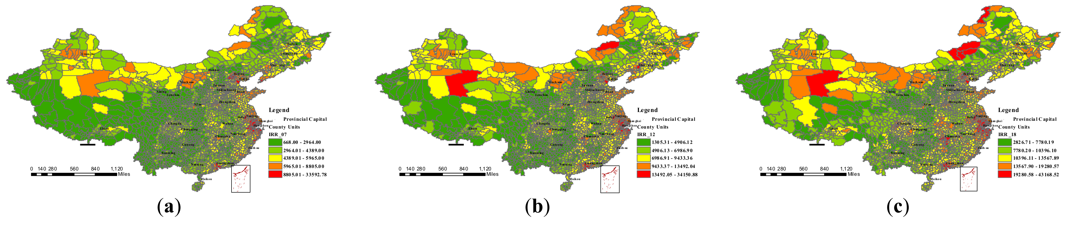
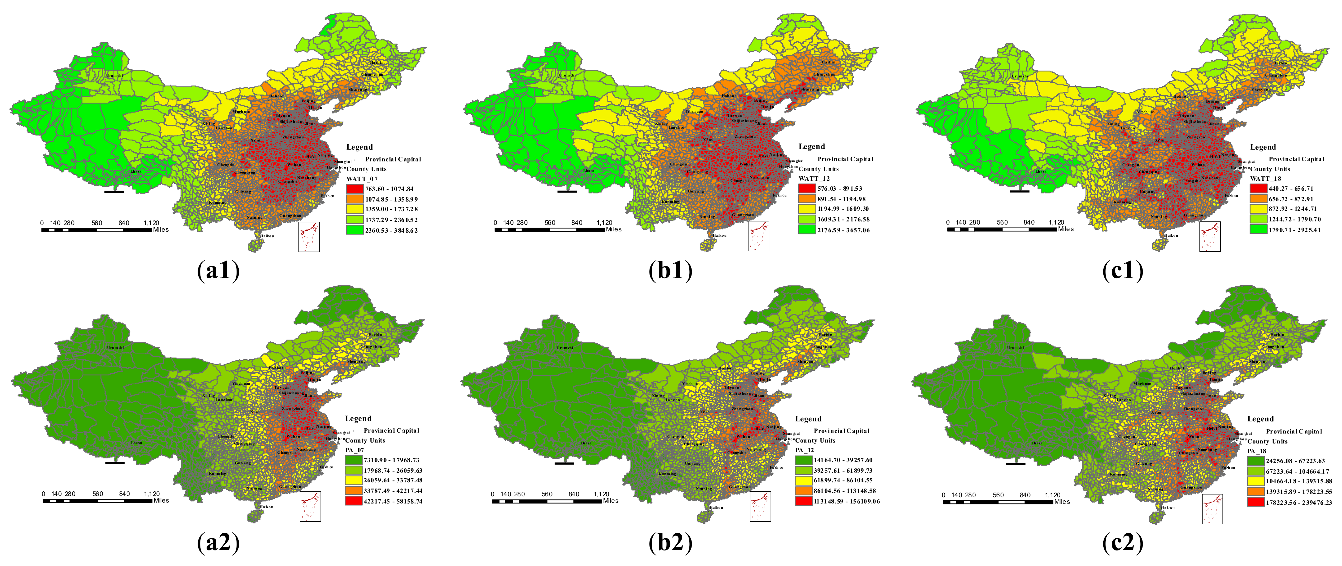
5.3. Spatial Distribution of Accessibility

Based on the travel time between each origin–destination pair, together with destination population and GDP data, the weighted average travel time and potential accessibility value were calculated for each of the 2341 counties.

Table 4. Descriptive statistics of accessibility indicators.

	2007			2012			2018
	Total	Poor	Non-Poor	Total	Poor	Non-Poor	Total	Poor	Non-Poor
WATT	1312 (0.37)	1511 (0.39)	1204 (0.30)	1072 (0.44)	1300 (0.46)	948 (0.35)	788 (0.45)	945 (0.49)	703 (0.33)
PA	30,197 (0.37)	24,193 (0.40)	33,471 (0.31)	71,520 (0.42)	54,590 (0.45)	80,751 (0.35)	126,169 (0.37)	100,655 (0.39)	140,079 (0.31)

Note: The coefficient of variation is in parentheses.

shows the mean value and coefficient of variation for WATT and PA in different sample groups. Accessibility progressively increased over 10 years during the study period. The WATT values for all counties decreased from 1312 to 788 min and PA increased from 30,197 to 126,169, reflecting a 39.9% and 317.8% increase in accessibility with HSR introduction. Poor counties were less accessible than non-poor counties. The WATT of poor counties in 2007 was 1.25 times that of non-poor counties and in 2018 was 1.34 times. For PA, the ratio between non-poor to poor counties increased from 1.38 in 2007 to 1.47 in 2012, then decreased to 1.39 in 2018. The relative gap of accessibility between poor and non-poor counties increased with HSR development at this stage.

Accessibility maps for the entire research scope shown in Figure 4 were built using an ArcGIS classification technique, namely natural breaks, ensuring the maximization of differences between levels. The color changed from red to green, with accessibility changing from high to low. In 2007, without HSR, the spatial distribution accessibility measured by WATT and PA exhibited significant “core-periphery” features from east to west. In 2018, corridor effects created by HSR development became more pronounced.

5.4. The Inequality of Rural Income and Accessibility

Table 5. Comparison of the Theil index between different groups.

		Total Counties	First Group Scheme			Second Group Scheme
			Poor	Non-Poor	Intra-Group	Inter-Group	Intra-Group	Inter-Group
TP-IRR	2007	0.3190	0.4410	0.2849	0.3172	0.0018	0.2307	0.0883
	2012	0.3217	0.4455	0.2864	0.3215	0.0002	0.2364	0.0853
	2018	0.3392	0.4562	0.2998	0.3384	0.0008	0.2448	0.0944
TP-WATT	2007	0.6525	0.7818	0.4376	0.5774	0.0751	0.2932	0.3593
	2012	0.7136	0.8088	0.4733	0.6168	0.0968	0.3011	0.4126
	2018	0.7351	0.8489	0.4941	0.6442	0.0909	0.3184	0.4167
TP-PA	2007	0.2583	0.2705	0.2439	0.2514	0.0069	0.2028	0.0556
	2012	0.2532	0.2698	0.2411	0.2488	0.0044	0.2014	0.0518
	2018	0.2617	0.2628	0.2515	0.2547	0.0071	0.2154	0.0463

and Appendix A present the outcomes of the Theil index calculation. Between 2007 and 2018, the disparity of IRR and WATT at the national level continued to increase, while the disparity of PA slightly decreased and then increased. Division of counties into poor and non-poor types revealed that the disparity of rural income and accessibility was larger among poor counties compared to non-poor counties. In particular, the decomposed result of the second group scheme shows that the intra-group index is larger than the inter-group index with respect to rural income and potential accessibility. This indicates the existence of social inequality among counties within specific provinces in China. Moreover, after grouping counties by province, it was found that the inter-group index of weighted average travel time was larger than the intra-group index. Therefore, the inter-province disparity of weighted average travel time was more significant. With the development of the HSR, the accessibility disparity increased, which is consistent with the results provided by Jiao et al. [5], while different provinces showed different performances. In Jiangsu province, the accessibility disparity decreased, which is consistent with research by Wang et al. [4]. The disparity in the accessibility of Liaoning province first decreased and then increased. Luo and Zhao [46] found that the disparity of railway accessibility was lower than that of highway accessibility in Liaoning province in 2016.

To examine the association between rural income disparity and accessibility disparity, Pearson correlation coefficients were calculated, with 31 provinces as observations. The results of the Pearson coefficient show that the Theil index of IRR is significantly positively correlated with the Theil index of PA and WATT. The three-year average value of Pearson coefficients between T_P-IRR and T_P-PA is 0.80 and for T_P-IRR and T_P-WATT the correlation is 0.83. This indicates that the inequality of accessibility is closely related to income disparity. To reduce the inequality of rural income, the government should focus on reducing disparities in accessibility between counties.

6. Accessibility and Poverty Reduction

6.1. Model Specification

• Two Way Fixed Effect Models

Based on the accessibility calculations before and after HSR was introduced into the railway system, the correlation between regional accessibility improvement and regional poverty reduction was analyzed in this study. The per capita income of rural residents is a representative variable measuring the absolute poverty level of a county [20]; and the ratio of rural income to urban income represents the relative poverty level. To empirically test the association between accessibility and absolute poverty or relative poverty, two baseline regression models are set as follows:

$$\begin{gathered} \mathrm{Model}1:lnIR{R}_{it}={\alpha }_0+{\alpha }_{1}lnP{A}_{it}+{\alpha }_{2}lnCPO{P}_{it}+{\alpha }_{3}lnPGD{P}_{it}+ \\ {\alpha }_{4}lnSP{G}_{it}+{\alpha }_{5}lnPIN{V}_{it}+{\alpha }_{6}lnPEOP{F}_{it}+{\alpha }_{7}lnPNE{P}_{it}+{\alpha }_{8}AF{F}_{it}+{\mu }_i+{\gamma }_t+{\epsilon }_{it} \end{gathered}$$

(6)

$$\begin{gathered} \mathrm{Model}2:lnRU{G}_{it}={\beta }_0+{\beta }_{1}lnP{A}_{it}+{\beta }_{2}lnCPO{P}_{it}+{\beta }_{3}lnPGD{P}_{it}+ \\ {\beta }_{4}lnSP{G}_{it}+{\beta }_{5}lnPIN{V}_{it}+{\beta }_{6}lnPEOP{F}_{it}+{\beta }_{7}lnPNE{P}_{it}+{\beta }_{8}AF{F}_{it}+{\mu }_i+{\gamma }_t+{\epsilon }_{it} \end{gathered}$$

(7)

where $i$ and $t$ represent the county and the year, respectively. In model 1, the dependent variable (lnIRR) represents the natural log of rural income. The core explanatory variable is the natural log of potential accessibility (lnPA). Other elements that may affect the rural income are controlled; these factors include (1) human capital, measured by the natural log of the county’s population (lnCPOP); (2) the level of local economic development, measured by the natural log of GDP per capita (lnPGDP); (3) economic structure, measured by the natural log of the share of production in the secondary industry (lnSPG); (4) investment in fixed assets, measured by the natural log of the fixed-asset investment per capita (lnPINV); (5) public finance expenditures, measured by the natural log of public finance expenditures per capita (lnPEOPF); (6) employment level, measured by the natural log of the proportion of employed individuals to the total population (lnPNEP); and (7) air transport, measured by daily flight frequency (AFF). Based on data availability, data for the control variables, including lnSPG, lnPINV, lnPEOPF, lnPNEP and AFF, are from the prefectural level administrative regions where that county is located. Furthermore, the county-fixed effect (${\mu }_i$) and the year fixed effect (${\gamma }_t$) are also controlled. The term ${\alpha }_0$ is a constant term and $\epsilon$ is an error term.

For model 2, the dependent variable is the natural log of the rural-urban income gap, which is measured by Equation (8). The control variables are the same as model 1:

$$RU{G}_{it}=\frac{IR{R}_{county i}}{IU{R}_{prefecture j}}$$

(8)

where $IR{R}_{county i}$ is the rural resident income of county $i$, and $IU{R}_{prefecture j}$ is the urban resident income of prefecture $j$. Prefecture $j$ has jurisdiction over county $i$. The value of RUG is less than 1. A larger RUG value is associated with a smaller rural-urban income gap.

Model 1 and model 2 are used for three parallel regressions for all counties, poor counties, and non-poor counties. Two robustness tests were conducted. One studies poor counties that only belong to contiguous poor areas (CPA) and another involves the selection of counties after deleting municipal districts as samples.

• Spatial Economic Models

The values of Moran’s I reveal a strong positive spatial correlation with IRR. Considering the presence of spatial autocorrelation, spatial regression models, including a spatial lag model (SAR), spatial error model (SEM) and a mix of SAR and SEM (SAC), are introduced. Building upon baseline Equations (6) and (7) and two-stage formulation (9) and (10), the following spatial economic models, involving spatial autocorrelation, are constructed:

$$\begin{array}{l}\mathrm{Model}3:lnIR{R}_{it}=\rho {\sum }_{j=1}^n{\omega }_{ij}lnIR{R}_{jt}+{\alpha }_0+{\alpha }_{1}lnP{A}_{it}+{\alpha }_{2}lnCPO{P}_{it}+\\ {\alpha }_{3}lnPGD{P}_{it}+{\alpha }_{4}lnSP{G}_{it}+{\alpha }_{5}lnPIN{V}_{it}+{\alpha }_{6}lnPEOP{F}_{it}+{\alpha }_{7}lnPNE{P}_{it}+\\ {\alpha }_{8}AF{F}_{it}+{\mu }_i+{\gamma }_t+{\epsilon }_{it}\\ {\epsilon }_{it}=\lambda {\displaystyle \sum _{j=1}^n}{\omega }_{ij}{\epsilon }_{jt}+v_{it}\end{array}$$

(9)

$$\begin{array}{l}\mathrm{Model}4:lnRU{G}_{it}=\rho {\sum }_{j=1}^n{\omega }_{ij}lnRU{G}_{jt}+{\beta }_0+{\beta }_{1}lnP{A}_{it}+{\beta }_{2}lnCPO{P}_{it}+\\ {\beta }_{3}lnPGD{P}_{it}+{\beta }_{4}lnSP{G}_{it}+{\beta }_{5}lnPIN{V}_{it}+{\beta }_{6}lnPEOP{F}_{it}+{\beta }_{7}lnPNE{P}_{it}+\\ {\beta }_{8}AF{F}_{it}+{\mu }_i+{\gamma }_t+{\epsilon }_{it}\\ {\epsilon }_{it}=\lambda {\displaystyle \sum _{j=1}^n}{\omega }_{ij}{\epsilon }_{jt}+v_{it}\end{array}$$

(10)

where ${\omega }_{ij}$ denotes the spatial weight matrix; $\rho$ represents the spatial autocorrelation effects in the dependent variables; $\lambda$ represents the spatial autocorrelation effects in the random error. If $\rho \ne 0 and \lambda =0$, the SAR model is estimated. If $\rho =0 and \lambda \ne 0$, the SEM model is estimated. If $\rho \ne 0 and \lambda \ne 0$, the SAC model is estimated.

Two types of spatial weight matrices are frequently used in spatial economic models. The first is the adjacency weight matrix, which includes dummy variables indicating whether counties are neighbors (1 represents neighbors and 0 otherwise). The second is the spatial distance matrix, constructed by using the inverse of the Euclidean distance between the counties’ government office buildings.

Table 6. Results of the Moran’s I.

Year	IRR		RUG
	Adjacency Weight Matrix	Spatial Distance Matrix	Adjacency Weight Matrix	Spatial Distance Matrix
2007	0.727 ***	0.506 ***	0.570 ***	0.368 ***
2012	0.728 ***	0. 496 ***	0.564 ***	0.360 ***
2018	0.747 ***	0.519 ***	0.544 ***	0.346 ***

Note: ***, **, and * indicate significance at 1, 5, and 10% levels, respectively.

lists Moran’s I of two dependent variables in this study calculated based on these two matrices. The values of Moran’s I together with the p-value indicate the existence of significant spatial autocorrelations in IRR and RUG and the spatial autocorrelation is higher based on the adjacency weight matrix. Therefore, the adjacency weight matrix was adopted in our spatial economic models.

6.2. Accessibility and Absolute Poverty Reduction

This subsection describes the estimated results of potential economic accessibility impact on absolute poverty reduction, by using two-way fixed effect models and spatial economic models. Considering the significant difference in accessibility and development level between poor and non-poor counties, the whole sample, the poor counties and the non-poor counties were regressed separately.

Table 7. The effect of accessibility on IRR (model 1).

	Different Groups of the Whole Sample				Different Groups after Deleting Municipal Districts
	(1)	(2)	(3)	(4)	(5)	(6)	(7)	(8)
	Total	Poor	CPA	Non-Poor	Total	Poor	CPA	Non-Poor
lnPA	0.1718 *** (0.0142)	0.2431 *** (0.0249)	0.2113 *** (0.0257)	0.1329 *** (0.0145)	0.1753 *** (0.0156)	0.2405 *** (0.0257)	0.2112 *** (0.0265)	0.1307 *** (0.0163)
lnPGDP	0.1505 *** (0.0150)	0.1013 *** (0.0246)	0.0749 *** (0.0258)	0.1434 *** (0.0164)	0.1500 *** (0.0162)	0.1018 *** (0.0254)	0.0776 *** (0.0267)	0.1474 *** (0.0184)
lnPINV	0.0153 ** (0.0064)	−0.0266 ** (0.0113)	−0.0357 *** (0.0119)	0.0354 *** (0.0065)	0.0122 * (0.0070)	−0.0234 ** (0.0115)	−0.0345 *** (0.0122)	0.0328 *** (0.0071)
lnSPG	−0.0153 (0.0205)	0.0419 (0.0279)	0.0357 (0.0301)	−0.0861 *** (0.0217)	−0.0153 (0.0222)	0.0381 (0.0288)	0.0339 (0.0313)	−0.0929 *** (0.0244)
lnPEOPF	0.1477 *** (0.0139)	0.1104 *** (0.0174)	0.0786 *** (0.0167)	0.0717 *** (0.0158)	0.1459 *** (0.0151)	0.1131 *** (0.0182)	0.0799 *** (0.0175)	0.0659 *** (0.0174)
lnPNEP	−0.0376 *** (0.0095)	−0.0662 *** (0.0190)	−0.0522 ** (0.0206)	−0.0091 (0.0089)	−0.0393 *** (0.0108)	−0.0698 *** (0.0207)	−0.0541 ** (0.0214)	−0.0059 (0.0098)
AFF	−0.0003 *** (0.0001)	−0.0002 ** (0.0001)	−0.0002 *** (0.0001)	−0.0002 *** (0.0001)	−0.0002 *** (0.0001)	−0.0002 ** (0.0001)	−0.0002 *** (0.0001)	−0.0001 (0.0001)
lnCPOP	0.0020 (0.0311)	−0.0349 (0.0404)	−0.0498 (0.0387)	−0.0326 (0.0400)	0.0256 (0.0361)	−0.0393 (0.0409)	−0.0523 (0.0392)	−0.0171 (0.0503)
cons	3.7032 *** (0.2470)	3.6258 *** (0.3483)	4.6269 *** (0.3675)	5.3265 *** (0.3191)	3.5331 *** (0.2704)	3.6200 *** (0.3536)	4.5933 *** (0.3744)	5.2924 *** (0.3774)
Year FE	fixed	fixed	fixed	fixed	fixed	fixed	fixed	fixed
County FE	fixed	fixed	fixed	fixed	fixed	fixed	fixed	fixed
R2	0.9547	0.9559	0.9610	0.9666	0.9539	0.9551	0.9602	0.9668
No. of Obs	7023	2478	2022	4545	6084	2397	1959	3687

Note: ***, **, and * indicate significance at 1, 5, and 10% levels, respectively. Robust standard errors clustered by county are shown in parentheses.

summarizes the results of two-way fixed effect models. For whole samples, the results show that potential economic accessibility improvement has a significant positive effect on rural income. The economic development level, investment in fixed assets and public finance expenditure also have a significant positive effect on rural income. In contrast, employment level and air transport (flight frequency) have a significant negative effect on rural income. Potential economic accessibility has a larger effect on rural income for poor counties, while the economic development level has a larger effect on non-poor counties. Rural residents in non-poor counties benefit from fixed asset investments, while residents in poor counties do not. The robustness of the results for comparing poor and non-poor counties is tested by taking poor counties located in continuous poor areas as samples. The results are summarized in column (3). After excluding 313 out of 2341 counties with more urbanized manuscript districts, the estimated coefficient of PA becomes larger for total counties. However, when grouping counties into poor and non-poor, if most urbanized districts are deleted, the influence coefficient becomes smaller. Overall, the impact of accessibility improvement on underdeveloped areas is greater than the agglomeration effect on developed areas. However, for different groups, the more developed districts have a larger agglomeration effect.

Table 8. The effect of accessibility on IRR (model 3).

	SAR			SEM			SAC
	(1)	(2)	(3)	(4)	(5)	(6)	(7)	(8)	(9)
	Total	Poor	Non-Poor	Total	Poor	Non-Poor	Total	Poor	Non-Poor
lnPA	0.0478 *** (0.0103)	0.0973 *** (0.0207)	0.0578 *** (0.0120)	0.0306 (0.0204)	0.1096 *** (0.0339)	0.0494 *** (0.0189)	0.0327 *** (0.0074)	0.0568 *** (0.0117)	0.0281 (0.0165)
lnPGDP	0.0611 *** (0.0112)	0.0626 *** (0.0192)	0.0800 *** (0.0147)	0.0964 *** (0.0218)	0.1146 *** (0.0329)	0.1110 *** (0.0217)	0.0404 *** (0.0084)	0.0324 *** (0.0107)	0.0927 *** (0.0163)
lnPINV	0.0003 (0.0050)	−0.0173 * (0.0100)	0.0137 ** (0.0053)	0.0065 (0.0096)	−0.0197 (0.0190)	0.0195 ** (0.0091)	−0.0025 (0.0036)	−0.0139 ** (0.0050)	0.0139 (0.0066)
lnSPG	0.0045 (0.0159)	0.0250 (0.0231)	−0.0474 ** (0.0184)	0.0263 (0.0273)	0.0256 (0.0387)	−0.0332 (0.0247)	0.0000 (0.0116)	0.0147 (0.0107)	−0.0234 (0.0166)
lnPEOPF	0.0528 *** (0.0094)	0.0604 *** (0.0148)	0.0407 *** (0.0130)	0.0509 *** (0.0156)	0.0772 *** (0.0225)	0.0383 * (0.0145)	0.0381 *** (0.0072)	0.0395 *** (0.0089)	0.0255 (0.0146)
lnPNEP	−0.0156** (0.0074)	−0.0337 ** (0.0168)	−0.0066 (0.0072)	−0.0216 ** (0.0119)	−0.0480* (0.0253)	−0.0105 (0.0086)	−0.0096 * (0.0055)	−0.0168 (0.0081)	−0.0102 (0.0086)
AFF	−0.0001 *** (0.0000)	−0.0001 ** (0.0001)	−0.0001 ** (0.0000)	−0.0002 *** (0.0001)	−0.0002 ** (0.0001)	−0.0001 (.0000)	−0.0001 *** (0.0000)	−0.0001 ** (0.0001)	−0.0001 (0.0000)
lnCPOP	−0.0318 (0.0309)	−0.0189 (0.0321)	−0.0355 (0.0392)	−0.0479 (0.0354)	−0.0133 (0.0377)	−0.0394 (.0146)	−0.0235 (0.0248)	−0.0254 (0.0179)	−0.0382 (0.0132)
λ				0.7224 *** (0.0132)	0.5835 *** (0.0286)	0.6242 *** (0.0190)	−0.4251 *** (0.0596)	−0.4969 *** (0.0843)	0.8186 *** (0.0703)
ρ	0.6963 *** (0.0128)	0.5987 *** (0.0166)	0.5490 *** (0.0272)				0.8291 *** (0.0149)	0.8128 *** (0.0270)	−0.5541 ** (0.2603)
Year FE	fixed	fixed	fixed	fixed	fixed	fixed	fixed	fixed	fixed
County FE	fixed	fixed	fixed	fixed	fixed	fixed	fixed	fixed	fixed
R2	0.9302	0.9239	0.9459	0.8933	0.9227	0.9318	0.9331	0.9172	0.9007
No. of Obs	7023	2478	4545	7023	2478	4545	7023	2478	4545

Note: ***, **, and * indicate significance at 1, 5, and 10% levels, respectively. Robust standard errors clustered by county are shown in parentheses.

summarizes the results estimated by using the three spatial economic models. In particular, spatial economic models indicate that conventional linear regression approaches may have overestimated the benefits by not considering the spatial autocorrelation of rural income. The values of the R-square indicate that the SAC model is appropriate for the whole sample, while the SAR model is appropriate for poor and non-poor subgroups. The results indicate that the potential accessibility improvement has rural income growth impacts with an overall elastic coefficient of 0.03; the coefficient is 0.10 for poor areas and 0.06 for non-poor areas.

6.3. Accessibility and Relative Poverty Reduction

Table 9. The effect of accessibility on RUG (model 2).

	Different Groups of the Whole Sample				Different Groups after Deleting Municipal Districts
	Total	Poor	Co-Poor	Non-Poor	Total	Poor	Co-Poor	Non-Poor
lnPA	0.1151 *** (0.0139)	0.1767 *** (0.0248)	0.1476 *** (0.0252)	0.0878 *** (0.0156)	0.1161 *** (0.0152)	0.1784 *** (0.0256)	0.1492 *** (0.0259)	0.0804 *** (0.0173)
lnPGDP	0.0715 *** (0.0150)	0.0209 (0.0235)	−0.0030 (0.0252)	0.0780 *** (0.0204)	0.0749 *** (0.0160)	0.0212 (0.0243)	−0.0008 (0.0262)	0.0918 *** (0.0224)
lnPINV	0.0174 ** (0.0067)	−0.0163 (0.0118)	−0.0222 * (0.0118)	0.0325 *** (0.0076)	0.0142 ** (0.0072)	−0.0132 (0.0120)	−0.0209 * (0.0121)	0.0286 *** (0.0082)
lnSPG	−0.0360 * (0.0198)	0.0043 (0.0282)	−0.0070 (0.0299)	−0.0890 *** (0.0258)	−0.0397 * (0.0212)	0.0032 (0.0290)	−0.0051 (0.0310)	−0.1056 *** (0.0284)
lnPEOPF	0.1090 *** (0.0122)	0.0973 *** (0.0179)	0.0662 *** (0.0188)	0.0424 ** (0.0183)	0.1113 *** (0.0131)	0.0977 *** (0.0189)	0.0641 *** (0.0199)	0.0432 ** (0.0203)
lnPNEP	−0.0303 *** (0.0097)	−0.0574 *** (0.0193)	−0.0396 ** (0.0199)	−0.0068 (0.0102)	−0.0358 *** (0.0108)	−0.0622 *** (0.0210)	−0.0416 ** (0.0208)	−0.0090 (0.0111)
AFF	−0.0003 *** (0.0001)	−0.0001 (0.0001)	−0.0001 (0.0001)	−0.0003 *** (0.0001)	−0.0002 *** (0.0001)	−0.0001 (0.0001)	−0.0001 (0.0001)	−0.0002 *** (0.0001)
lnCPOP	0.0255 (0.0299)	−0.0419 (0.0423)	−0.0845 ** (0.0390)	0.0278 (0.0390)	0.0283 (0.0347)	−0.0512 (0.0428)	−0.0902 ** (0.0396)	0.0263 (0.0499)
cons	−4.066 *** (0.2346)	−3.978 *** (0.3451)	−2.8856 *** (0.3440)	−3.0763 *** (0.3218)	−4.142 *** (0.2532)	−3.9919 *** (0.3509)	−2.905 *** (0.3492)	−3.0537 *** (0.3769)
Year FE	fixed	fixed	fixed	fixed	fixed	fixed	fixed	fixed
County FE	fixed	fixed	fixed	fixed	fixed	fixed	fixed	fixed
R2	0.5496	0.6569	0.7067	0.4886	0.5604	0.6554	0.7041	0.4989
No. of Obs	7023	2478	2022	4545	6084	2397	1959	3687

Note: ***, **, and * indicate significance at 1, 5, and 10% levels, respectively. Robust standard errors clustered by county are shown in parentheses.

and

Table 10. The effect of accessibility on RUG (model 4).

	SAR			SEM			SAC
	Total	Poor	Non-Poor	Total	Poor	Non-Poor	Total	Poor	Non-Poor
lnPA	0.0391 *** (0.0106)	0.0872 *** (0.0207)	0.0336 *** (0.0117)	0.0373 * (0.0202)	0.1014 *** (0.0332)	0.0344 * (0.0196)	0.0279 *** (0.0077)	0.0507 *** (0.0126)	0.0159 (0.0199)
lnPGDP	0.0228 * (0.0117)	0.0057 (0.0196)	0.0317 ** (0.0160)	0.0192 (0.0229)	−0.0079 (0.0339)	0.0465 * (0.0244)	0.0161 * (0.0085)	0.0038 (0.0118)	0.0401 (0.0249)
lnPINV	0.0030 (0.0053)	−0.0084 (0.0108)	0.0095 * (0.0056)	0.0068 (0.0102)	−0.0039 (0.0200)	0.0078 (0.0106)	−0.0002 (0.0038)	−0.0060 (0.0063)	0.0006 (0.0113)
lnSPG	−0.0145 (0.0151)	−0.0006 (0.0227)	−0.0505 *** (0.0192)	−0.0149 (0.0264)	−0.0064 (0.0374)	−0.0642 ** (0.0264)	−0.0111 (0.0110)	−0.0015 (0.0140)	−0.0564** (0.0252)
lnPEOPF	0.0411 *** (0.0095)	0.0571 *** (0.0149)	0.0222 (0.0137)	0.0365 ** (0.0164)	0.0696 *** (0.0234)	0.0281 (0.0229)	0.0308 *** (0.0071)	0.0357 *** (0.0098)	0.0232 (0.0233)
lnPNEP	−0.0097 (0.0076)	−0.0308 * (0.0174)	−0.0009 (0.0076)	−0.0105 (0.0118)	−0.0435* (0.0251)	−0.0034 (0.0113)	−0.0061 (0.0056)	−0.0144 (0.0104)	−0.0043 (0.0108)
AFF	−0.0002 *** (0.0000)	−0.0000 (0.0001)	−0.0002 *** (0.0000)	−0.0002 *** (0.0001)	0.0000 (0.0001)	−0.0002 *** (0.0001)	−0.0001 *** (0.0000)	−0.0000 (0.0001)	−0.0002 *** (0.0001)
lnCPOP	−0.0233 (0.0295)	−0.0426 (0.0335)	−0.0050 (0.0379)	−0.0538 (0.0334)	−0.0581 (0.0392)	−0.0221 (0.0381)	−0.0135 (0.0239)	−0.0299 (0.0227)	−0.0232 (0.0341)
λ				0.7138 *** (0.0130)	0.5481 *** (0.0295)	0.6757 *** (0.0164)	−0.4146 *** (0.0545)	−0.5321 *** (0.0785)	0.8500 *** (0.0526)
ρ	0.6995 *** (0.0127)	0.5462 *** (0.0306)	0.6598 *** (0.0166)				0.8320 *** (0.0146)	0.7944 *** (0.0244)	−0.5416 *** (0.0143)
Year FE	fixed	fixed	fixed	fixed	fixed	fixed	fixed	fixed	fixed
County FE	fixed	fixed	fixed	fixed	fixed	fixed	fixed	fixed	fixed
R2	0.4955	0.6075	0.4419	0.4897	0.6060	0.4475	0.4947	0.6048	0.4343
No. of Obs	7023	2478	4545	7023	2478	4545	7023	2478	4545

Note: ***, **, and * indicate significance at 1, 5, and 10% levels, respectively. Robust standard errors clustered by county are shown in parentheses.

present the estimated results of models 2 and 4, respectively. The results indicate that improving potential economic accessibility effectively narrowed the urban–rural income gap, with the benefits accruing more to poor counties compared to non-poor counties. Based on provincial panel data, Wei and Bu [27] also found that HSR could narrow the urban–rural income gap and the effect on the income of rural residents is greater than that of urban residents. The economic development level has a significant positive effect on the increase in the ratio of rural income to urban income for whole samples and non-poor counties. Public finance expenditures have a significant positive effect on whole samples and poor counties. The frequency of flights has a modest negative effect on the ratio of rural income to urban income for whole samples and for non-poor counties.

6.4. Further Robustness Tests

Following the main analyses, additional robustness tests were conducted to verify the effectiveness of the results of spatial economic models. The first tests addressed concerns about the accessibility measure. In models 3 and 4, lnPA was changed into the natural log of weighted average travel time (lnWATT) as the independent variable to verify the impact of accessibility improvement on poverty reduction. The model consisted of absolute poverty, measured by rural income, and relative poverty, measured by the ratio of rural income to urban income. The results reported in

Table 11. Results of robustness test.

Spatial Weight Matrix	Adjacency Weight Matrix						Spatial Distance Matrix
Dependent Variables	lnIRR			lnRUG			lnIRR	lnRUG
	(1)	(2)	(3)	(4)	(5)	(6)	(7)	(8)
	Total	Poor	Non-Poor	Total	Poor	Non-Poor	Total	Total
lnWATT	−0.0289 *** (0.0097)	−0.1083 *** (0.0266)	−0.0514 *** (0.0166)	−0.0312 ** (0.0145)	−0.0883 *** (0.0271)	−0.0342 *** (0.0165)
lnPA							0.0385 *** (0.0103)	0.0366 *** (0.0113)
Controlled	Yes	Yes	Yes	Yes	Yes	Yes	Yes	Yes
$\mathsf{\lambda }$	−0.4317 *** (0.0595)						−0.0802 (0.1001)
$\mathsf{\rho }$	0.8343 *** (0.0144)	0.6038 *** (0.0358)	0.5570 *** (0.0265)	0.7023 *** (0.0126)	0.5488 *** (0.0304)	0.6608 *** (0.0164)	0.9418 *** (0.0190)	0.9318 *** (0.0144)
Year FE	fixed	fixed	fixed	fixed	fixed	fixed	fixed	fixed
County FE	fixed	fixed	fixed	fixed	fixed	fixed	fixed	fixed
R2	0.9306	0.9232	0.9418	0.5029	0.6198	0.4538	0.9274	0.4691
No. of Obs	7023	2478	4545	7023	2478	4545	7023	7023

Note: ***, **, and * indicate significance at 1, 5, and 10% levels, respectively. Robust standard errors clustered by county are shown in parentheses.

(columns 1–3 and 4–6) indicate that a 1% decrease in weighted average travel time contributes to an overall increase in rural income and an increase in the ratio of rural–urban income by 0.0289% and 0.0312%, respectively, 0.1083% and 0.0883% for poor counties, respectively, and 0.0514% and 0.0342% for non-poor counties, respectively.

Second, after replacing the adjacency weight matrix with the spatial distance matrix in models 3 and 4, Table 11 (columns 7 and 8) shows the estimated results for the effects of potential economic accessibility on rural income and the ratio of rural income to urban income for total samples. Potential economic accessibility improvement has a significant and positive effect on poverty reduction, which is consistent with the results obtained with the adjacency weight matrix.

7. Discussion

The development of HSR has significantly reduced inter-county travel time, leading to improvement in the potential economic accessibility. The accessibility improvements have created significant development opportunities for poor counties and contiguous poor areas. In the context of poverty reduction goals, it is important to ensure that the poor can benefit from the advantages created by HSR expansion. This analysis indicates that improving accessibility has a positive effect on reducing both absolute poverty and relative poverty. One of the reasons is that the operation of high-speed railways, which are passenger-dedicated railway lines with high service efficiency, frees up the transport capacity of the conventional railway to transport agricultural products. Rural residents reap the benefits from saving transport costs including money and time and improving transport efficiency. Moreover, the success of HSR development in regional poverty reduction may be partly due to the other TPA strategies in China. When upgrading the local transportation infrastructure, the government also coordinates this activity with adjustments and upgrades to the local industrial structure, maximizing the regional advantages of industries and tourism and maintaining relevant skills training for low-income populations to protect the backward region from the siphoning effect.

Compared with the increase in rural income and decrease in the urban–rural income gap, rural income disparity increased at a national level. This is attributed to the fact that the rural income disparity between poor counties and counties within a single province became larger. Therefore, reducing the development difference between counties should be the goal of future investments. When developing poverty-alleviation-oriented policies, it is important to consider the poverty level and geographical characteristics of each county to implement diverse, fair and reasonable investment strategies. Ending regional poverty should go forward hand in hand with reducing inequality by utilizing strategies for improving transportation, public welfare, adjustment of the industrial structure, etc., and attaching importance to the Development Capacity Building of the nation, province, prefecture and county.

8. Conclusions

After eliminating the impact of price factors, the income of rural residents increased by 2.69 times from 4064 yuan (RMB) in 2007 to 10,951 yuan (RMB) in 2018 and the urban–rural income gap continued to decline. Significant progress was made in reducing poverty. However, the rural income disparity increased for both intra-group and inter-group measures. With the expansion of the HSR network, the accessibility measured by weighted average travel time decreased by 39.9% and the potential economic accessibility increased by 317.8%. However, the inequities of accessibility continued to rise, which is consistent with the result presented in a literature study [5]. Moreover, a strong positive correlation between rural income disparity and accessibility disparity indicates that the government should further address sustainable and balanced societal development. Based on the accessibility analysis, the effect on poverty reduction brought by accessibility improvement was further examined by using two-way fixed effect models and spatial economic models. In particular, when estimating the absolute poverty reduction effect, the goodness of fit test (R-square) of the spatial economic models indicates that SAC is a feasible method for total samples, while SAR is more suitable for subgroups, namely poor counties and non-poor counties. The SAR model is more suitable for estimating the relative poverty reduction effect. The empirical results show that a 1% improvement in the potential economic accessibility led to an improvement in the aggregated rural income by 0.03–0.17%. The ratio of rural income to urban income increased by 0.04–0.12%; for every 1% decrease in the weighted average travel time, rural income increased by 0.03%. The ratio of rural income to urban income increased by 0.02% and there was a larger effect in poor counties. Owing to spatial autocorrelation, the spatial economic model based on the adjacency weight matrix is better for exploring the association between regional poverty and accessibility.

In China, HSR development affects the income of rural residents and the urban–rural income gap by enhancing potential economic accessibility and reducing the weighted average travel time. This empirical research provides evidence that HSR development has broad poverty reduction effects in China’s anti-poverty initiatives. This can inform future poverty-alleviation-oriented transport policies. Based on experience gained from China’s anti-poverty initiatives, it is important to integrate transport policy with other anti-poverty strategies to accelerate sustainable development in poverty-stricken areas.

The improvement of railway accessibility is conducive to increase in rural income. However, the inequality of rural income and accessibility between counties increases, which may strengthen other facets of relative poverty problems. Therefore, it is urgent to solve the relative poverty by improving accessibility and alleviating accessibility disparities, which is the main goal of future national comprehensive transportation planning and transportation investments.

The relationships among accessibility brought by HSR development, regional poverty and inequality were explored at the macro-level in this study. The analysis conclusions are relatively weak in supporting micro policies for individuals. Moreover, research on the impact of HSR construction and operation on the environment is also meaningful, such as pollution emission and ecological conservation along HSR lines. The development of HSR receives widespread favor from the local government due to its high speed, large volume, high security, convenience and comfort. Comprehensive understanding of the cost of the HSR system and its positive or negative impact on the economy and the environment helps to rationally lay out HSR and eventually to realize the SDGs on schedule.

References

1. Nations, U. Transforming our world: The 2030 Agenda for Sustainable Development. Available online: https://sdgs.un.org/2030agenda (accessed on 17 September 2022).
2. Gannon, C.A.; Liu, Z. Poverty and Transport; World Bank: Washington, DC, USA, 1997. [Google Scholar]
3. Njenga, P.; Davis, A. Drawing the road map to rural poverty reduction. Transp. Rev. 2003, 23, 217–241. [Google Scholar] [CrossRef]
4. Wang, L.; Liu, Y.; Sun, C.; Liu, Y. Accessibility Impact of the present and future high-speed rail network: A case study of Jiangsu Province, China. J. Transp. Geogr. 2016, 54, 161–172. [Google Scholar] [CrossRef]
5. Jiao, J.; Wang, J.; Jin, F.; Dunford, M. Impacts on accessibility of China’s present and future HSR network. J. Transp. Geogr. 2014, 40, 123–132. [Google Scholar] [CrossRef]
6. Fan, J.; Li, Y.; Zhang, Y.; Luo, X.; Ma, C. Connectivity and accessibility of the railway network in China: Guidance for spatial balanced development. Sustainability 2019, 11, 7099. [Google Scholar] [CrossRef] [Green Version]
7. Jin, M.; Lin, K.-C.; Shi, W.; Lee, P.T.; Li, K.X. Impacts of high-speed railways on economic growth and disparity in China. Transp. Res. Part A: Policy Pract. 2020, 138, 158–171. [Google Scholar] [CrossRef]
8. Jia, S.; Zhou, C.; Qin, C. No difference in effect of high-speed rail on regional economic growth based on match effect perspective? Transp. Res. Part A: Policy Pract. 2017, 106, 144–157. [Google Scholar] [CrossRef]
9. Monzón, A.; Ortega, E.; López, E. Efficiency and spatial equity impacts of high-speed rail extensions in urban areas. Cities 2013, 30, 18–30. [Google Scholar] [CrossRef] [Green Version]
10. Monzon, A.; Lopez, E.; Ortega, E. Has HSR improved territorial cohesion in Spain? An accessibility analysis of the first 25 years: 1990–2015. Eur. Plan. Stud. 2019, 27, 513–532. [Google Scholar] [CrossRef]
11. Cascetta, E.; Cartenì, A.; Henke, I.; Pagliara, F. Economic growth, transport accessibility and regional equity impacts of high-speed railways in Italy: Ten years ex post evaluation and future perspectives. Transp. Res. Part A Policy Pract. 2020, 139, 412–428. [Google Scholar] [CrossRef]
12. Liu, S.; Wan, Y.; Zhang, A. Does China’s high-speed rail development lead to regional disparities? A network perspective. Transp. Res. Part A Policy Pract. 2020, 138, 299–321. [Google Scholar] [CrossRef]
13. Long, F.; Zheng, L.; Song, Z. High-speed rail and urban expansion: An empirical study using a time series of nighttime light satellite data in China. J. Transp. Geogr. 2018, 72, 106–118. [Google Scholar] [CrossRef]
14. Shao, S.; Tian, Z.; Yang, L. High speed rail and urban service industry agglomeration: Evidence from China’s Yangtze River Delta region. J. Transp. Geogr. 2017, 64, 174–183. [Google Scholar] [CrossRef]
15. Pagliara, F.; Mauriello, F. Modelling the impact of High Speed Rail on tourists with Geographically Weighted Poisson Regression. Transp. Res. Part A Policy Pract. 2020, 132, 780–790. [Google Scholar] [CrossRef]
16. Luis Campa, J.; Eugenia Lopez-Lambas, M.; Guirao, B. High speed rail effects on tourism: Spanish empirical evidence derived from China’s modelling experience. J. Transp. Geogr. 2016, 57, 44–54. [Google Scholar] [CrossRef]
17. Ren, X.; Chen, Z.; Wang, F.; Dan, T.; Wang, W.; Guo, X.; Liu, C. Impact of high-speed rail on social equity in China: Evidence from a mode choice survey. Transp. Res. Part A Policy Pract. 2020, 138, 422–441. [Google Scholar] [CrossRef]
18. Wu, L.; Jiang, Y.; Yang, F. The impact of high speed railway on government expenditure on poverty alleviation in China —Evidence from Chinese poverty counties. J. Asia Pac. Econ. 2022, 1–21. [Google Scholar] [CrossRef]
19. Liang, Y.; Zhou, K.; Li, X.; Zhou, Z.; Sun, W.; Zeng, J. Effectiveness of high-speed railway on regional economic growth for less developed areas. J. Transp. Geogr. 2020, 82, 102621. [Google Scholar] [CrossRef]
20. Park, A.; Wang, S.; Wu, G. Regional poverty targeting in China. J. Public Econ. 2002, 86, 123–153. [Google Scholar] [CrossRef]
21. Zhou, Y.; Guo, Y.; Liu, Y. Comprehensive measurement of county poverty and anti-poverty targeting after 2020 in China. Acta Geogr. Sin 2018, 73, 1478–1493. [Google Scholar]
22. Anyanwu, J.C.; Erhijakpor, A.E. The impact of road infrastructure on poverty reduction in Africa. In Poverty in Africa; Nova Science Publishers, Inc.: New York, NY, USA, 2009; pp. 1–40. [Google Scholar]
23. Fan, S.; Chan-Kang, C. Road Development, Economic Growth, and Poverty Reduction in China; International Food Policy Research Institute: Washington, DC, USA, 2005; Volume 12. [Google Scholar]
24. Narayan-Parker, D. Empowerment and Poverty Reduction: A Sourcebook; World Bank Publications: Washington, DC, USA, 2002. [Google Scholar]
25. Chen, Z.; Haynes, K.E. Impact of high-speed rail on regional economic disparity in China. J. Transp. Geogr. 2017, 65, 80–91. [Google Scholar] [CrossRef]
26. Fan, J.; Kato, H.; Yang, Z.; Li, Y. Effects From Expanding High-Speed Railway Network on Regional Accessibility and Economic Productivity in China. Transp. Res. Rec. 2022, 2676, 145–160. [Google Scholar] [CrossRef]
27. Wei, L.; Bu, W. Does the High-speed Railway Reduce the Urban-rural Income Gap? In Proceedings of the 2018 5th International Conference on Industrial Economics System and Industrial Security Engineering (IEIS), Toronto, ON, Canada, 3–6 August 2018; IEEE: Toronto, ON, Canada, 2018; pp. 1–4. [Google Scholar]
28. The passenger volume of high-speed railway in China over the years. Available online: https://m.shujujidi.com/hangye/55.html (accessed on 3 October 2022).
29. Benevenuto, R.; Caulfield, B. Poverty and transport in the global south: An overview. Transp. Policy 2019, 79, 115–124. [Google Scholar] [CrossRef]
30. Ornati, O.A.; Whittaker, J.W.; Solomon, R. Transportation Needs of the Poor: A Case Study of New York City; Praeger: New York, NY, USA, 1969. [Google Scholar]
31. Idei, R.; Kato, H.; Morikawa, S. Contribution of rural roads improvement on children’s school attendance: Evidence in Cambodia. Int. J. Educ. Dev. 2020, 72, 102131. [Google Scholar] [CrossRef]
32. Idei, R.; Kato, H. Changes in individual economic activities and regional market structures caused by rural road improvements in Cambodia. Transp. Res. Rec. 2018, 2672, 26–36. [Google Scholar] [CrossRef]
33. Takada, S.; Morikawa, S.; Idei, R.; Kato, H. Impacts of improvements in rural roads on household income through the enhancement of market accessibility in rural areas of Cambodia. Transportation 2021, 48, 2857–2881. [Google Scholar] [CrossRef]
34. Zhao, P.; Yu, Z. Rural poverty and mobility in China: A national-level survey. J. Transp. Geogr. 2021, 93, 103083. [Google Scholar] [CrossRef]
35. Warr, P. Road Development and Poverty Reduction: The Case of Lao PDR; ADBI Research Paper Series: Tokyo, Japan, 2005. [Google Scholar]
36. Zou, W.; Zhang, F.; Zhuang, Z.; Song, H. Transport Infrastructure, Growth, and Poverty Alleviation: Empirical Analysis of China. Ann. Econ. Financ. 2008, 9, 345–371. [Google Scholar]
37. Yang, D.; Song, W. Does the Accessibility of Regional Internal and External Traffic Play the Same Role in Achieving Anti-Poverty Goals? Land 2022, 11, 90. [Google Scholar] [CrossRef]
38. Cartenì, A.; Pariota, L.; Henke, I. Hedonic value of high-speed rail services: Quantitative analysis of the students’ domestic tourist attractiveness of the main Italian cities. Transp. Res. Part A Policy Pract. 2017, 100, 348–365. [Google Scholar] [CrossRef]
39. Farrington, J.; Farrington, C. Rural accessibility, social inclusion and social justice: Towards conceptualisation. J. Transp. Geogr. 2005, 13, 1–12. [Google Scholar] [CrossRef]
40. Murakami, J.; Cervero, R. High-Speed Rail and Economic Development: Business Agglomerations and Policy Implications; Routledge: London, UK, 2017. [Google Scholar]
41. Givoni, M. Development and impact of the modern high-speed train: A review. Transp. Rev. 2006, 26, 593–611. [Google Scholar] [CrossRef]
42. Garmendia, M.; de Urena, J.M.; Ribalaygua, C.; Leal, J.; Coronado, J.M. Urban residential development in isolated small cities that are partially integrated in metropolitan areas by high speed train. Eur. Urban Reg. Stud. 2008, 15, 249–264. [Google Scholar] [CrossRef]
43. Liu, S.; Kesteloot, C. High-Speed Rail and Rural Livelihood: The Wuhan-Guangzhou Line and Qiya Village. Tijdschr. Voor Econ. En Soc. Geogr. 2016, 107, 468–483. [Google Scholar] [CrossRef]
44. Li, W.; Wang, X.; Hilmola, O.-P. Does High-Speed Railway Influence Convergence of Urban-Rural Income Gap in China? Sustainability 2020, 12, 4236. [Google Scholar] [CrossRef]
45. The operating mileage of high-speed railway in China over the years. Available online: https://m.shujujidi.com/hangye/54.html (accessed on 3 October 2022).
46. Luo, H.; Zhao, S. Impacts of high-speed rail on the inequality of intercity accessibility: A case study of Liaoning Province, China. J. Transp. Geogr. 2021, 90, 102920. [Google Scholar] [CrossRef]
47. Kun, Y. Poverty Alleviation in China; Springer-Verlag: Berlin, Germany, 2016. [Google Scholar]
48. Bank, W. China—Systematic Country Diagnostic: Towards a More Inclusive and Sustainable Development; World Bank Group: Washington, DC, USA, 2018. [Google Scholar]
49. Domma, F.; Condino, F.; Giordano, S. A new formulation of the Dagum distribution in terms of income inequality and poverty measures. Phys. A: Stat. Mech. Its Appl. 2018, 511, 104–126. [Google Scholar] [CrossRef]
50. Yin, M.; Bertolini, L.; Duan, J. The effects of the high-speed railway on urban development: International experience and potential implications for China. Prog. Plan. 2015, 98, 1–52. [Google Scholar] [CrossRef] [Green Version]
51. Li, Y.; Fan, J.; Deng, H. Analysis of regional difference and correlation between highway traffic development and economic development in China. Transp. Res. Rec. 2018, 2672, 12–25. [Google Scholar] [CrossRef]
52. Fisher, G.R.; Theil, H. Economics and Information Theory. J. R. Stat. Soc. Ser. A 1970, 133, 489. [Google Scholar] [CrossRef]
Figure 1. Poverty alleviation over time in China.
Land 11 01846 g001
Figure 2. The spatial distribution of rural income during the three study years. (a) IRR of 2007; (b) IRR of 2012; (c) IRR of 2018.
Land 11 01846 g002
Figure 3. The spatial distribution of poor areas and HSR in China. (a) The Chinese HSR network from 2008 to 2018; (b) The distribution of poor counties; (c) The distribution of 14 contiguous poor areas.
Land 11 01846 g003
Figure 4. The spatial distribution of accessibility in the study years. (a1) WATT of 2007; (b1) WATT of 2012; (c1) WATT of 2018; (a2) PA of 2007; (b2) PA of 2012; (c2) PA of 2018.
Land 11 01846 g004