

Estimating Groundnut Yield in Smallholder Agriculture Systems Using PlanetScope Data
 , , , ,
Abstract
:1. Introduction
2. Materials and Methods
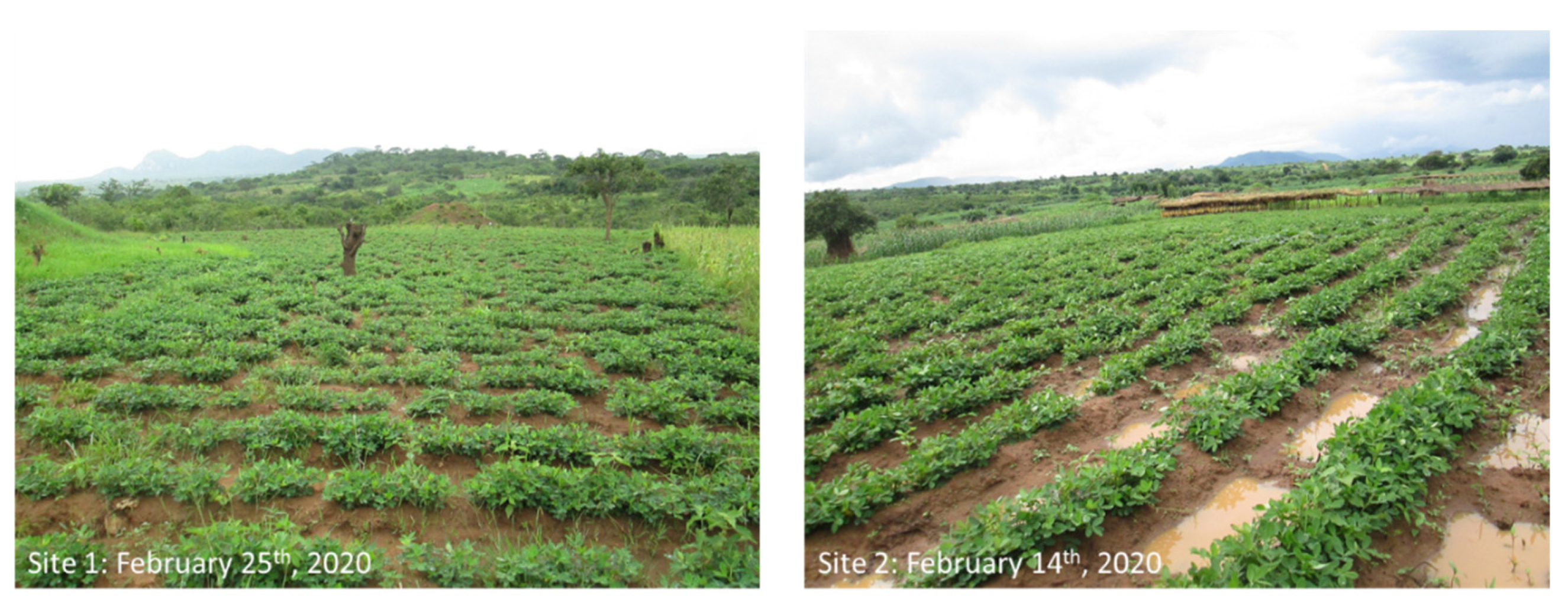
2.1. Study Sites
2.2. Study Design
3. Data Collection and Processing
3.1. Digital Hemispherical Photographs’ Capture and Processing
3.2. Groundnut Yield Data
3.3. Satellite Image Acquisition and Vegetation Index Selection
4. Analytical Approach
5. Results
5.1. Descriptive Statistics for Yield and In Situ LAI Data
5.2. Relationship between Average Observed Yield and Predictor Variables
6. Discussion
7. Conclusions
Author Contributions
Funding
Data Availability Statement
Conflicts of Interest
References
- USDA. World Agricultural Production; USDA: Washington, DC, USA, 2020. [Google Scholar]
- Nautiyal, P.C. Groundnut: Post-Harvest Operations. Res. Cent. Groundn. ICAR 2002, 23, 2013. [Google Scholar]
- Sako, D.; Traoré, M.; Doumbia, F.; Diallo, F.; Fané, M.; Kapran, I. Kolokani Groundnut Innovation Platform Activities and Achievements through TL III Project in Mali. In Enhancing Smallholder Farmers’ Access to Seed of Improved Legume Varieties through Multi-Stakeholder Platforms; Springer: Singapore, 2021; pp. 51–64. [Google Scholar]
- Aransiola, E.F.; Ehinmitola, E.O.; Adebimpe, A.I.; Shittu, T.D.; Solomon, B.O. Prospects of Biodiesel Feedstock as an Effective Ecofuel Source and Their Challenges. In Advances in Eco-Fuels for a Sustainable Environment; Elsevier: Amsterdam, The Netherlands, 2019; pp. 53–87. [Google Scholar]
- Corporate, C.A.I. Malawi Groundnut Outlook; Lilongwe, Malawi, 2016. Available online: https://mitc.mw/trade/index.php/groundnuts-export-product (accessed on 15 September 2022).
- Abady, S.; Shimelis, H.; Janila, P.; Mashilo, J. Groundnut (Arachis hypogaea L.) Improvement in Sub-Saharan Africa: A Review. Acta Agric. Scand. Sect. B-Soil Plant Sci. 2019, 69, 528–545. [Google Scholar]
- AICC. Harmonized Groundnut Production Manual for Malawi; Legumes Development Trust: Lilongwe, Malawi, 2014. [Google Scholar]
- Holzman, M.E.; Rivas, R.; Piccolo, M.C. Estimating Soil Moisture and the Relationship with Crop Yield Using Surface Temperature and Vegetation Index. Int. J. Appl. Earth Obs. Geoinf. 2014, 28, 181–192. [Google Scholar] [CrossRef]
- Schwalbert, R.A.; Amado, T.; Corassa, G.; Pott, L.P.; Prasad, P.V.V.; Ciampitti, I.A. Satellite-Based Soybean Yield Forecast: Integrating Machine Learning and Weather Data for Improving Crop Yield Prediction in Southern Brazil. Agric. For. Meteorol. 2020, 284, 107886. [Google Scholar] [CrossRef]
- WFP. Prevention of Undernutrition: 2019-Malawi Factsheets; WFP: Rome, Italy, 2019. [Google Scholar]
- Gao, F.; Anderson, M.; Daughtry, C.; Johnson, D. Assessing the Variability of Corn and Soybean Yields in Central Iowa Using High Spatiotemporal Resolution Multi-Satellite Imagery. Remote Sens. 2018, 10, 1489. [Google Scholar] [CrossRef] [Green Version]
- Thenkabail, P.S.; Knox, J.W.; Ozdogan, M.; Gumma, M.K.; Congalton, R.G.; Wu, Z.; Milesi, C.; Finkral, A.; Marshall, M.; Mariotto, I. Assessing Future Risks to Agricultural Productivity, Water Resources and Food Security: How Can Remote Sensing Help? Photogramm. Eng. Remote Sens. 2012, 78, 773–782. [Google Scholar]
- da Silva, E.E.; Baio, F.H.R.; Teodoro, L.P.R.; da Silva Junior, C.A.; Borges, R.S.; Teodoro, P. UAV-Multispectral and Vegetation Indices in Soybean Grain Yield Prediction Based on in Situ Observation. Remote Sens. Appl. Soc. Environ. 2020, 18, 100318. [Google Scholar] [CrossRef]
- Vergara-Díaz, O.; Zaman-Allah, M.A.; Masuka, B.; Hornero, A.; Zarco-Tejada, P.; Prasanna, B.M.; Cairns, J.E.; Araus, J.L. A Novel Remote Sensing Approach for Prediction of Maize Yield under Different Conditions of Nitrogen Fertilization. Front. Plant Sci. 2016, 7, 666. [Google Scholar] [CrossRef] [PubMed] [Green Version]
- Bolton, D.K.; Friedl, M.A. Forecasting Crop Yield Using Remotely Sensed Vegetation Indices and Crop Phenology Metrics. Agric. For. Meteorol. 2013, 173, 74–84. [Google Scholar] [CrossRef]
- Swain, K.C.; Thomson, S.J.; Jayasuriya, H.P.W. Adoption of an Unmanned Helicopter for Low-Altitude Remote Sensing to Estimate Yield and Total Biomass of a Rice Crop. Trans. ASABE 2010, 53, 21–27. [Google Scholar] [CrossRef] [Green Version]
- Wang, J.; Zhang, J.; Bai, Y.; Zhang, S.; Yang, S.; Yao, F. Integrating Remote Sensing-Based Process Model with Environmental Zonation Scheme to Estimate Rice Yield Gap in Northeast China. Field Crops Res. 2020, 246, 107682. [Google Scholar] [CrossRef]
- Stepanov, A.; Dubrovin, K.; Sorokin, A.; Aseeva, T. Predicting Soybean Yield at the Regional Scale Using Remote Sensing and Climatic Data. Remote Sens. 2020, 12, 1936. [Google Scholar] [CrossRef]
- Gómez, D.; Salvador, P.; Sanz, J.; Casanova, J.L. Potato Yield Prediction Using Machine Learning Techniques and Sentinel 2 Data. Remote Sens. 2019, 11, 1745. [Google Scholar] [CrossRef]
- Hunt, E.R.; Horneck, D.A.; Spinelli, C.B.; Turner, R.W.; Bruce, A.E.; Gadler, D.J.; Brungardt, J.J.; Hamm, P.B. Monitoring Nitrogen Status of Potatoes Using Small Unmanned Aerial Vehicles. Precis. Agric. 2018, 19, 314–333. [Google Scholar] [CrossRef]
- Xue, J.; Su, B. Significant Remote Sensing Vegetation Indices: A Review of Developments and Applications. J. Sens. 2017, 2017, 1353691. [Google Scholar] [CrossRef] [Green Version]
- Gitelson, A.A.; Peng, Y.; Arkebauer, T.J.; Suyker, A.E. Productivity, Absorbed Photosynthetically Active Radiation, and Light Use Efficiency in Crops: Implications for Remote Sensing of Crop Primary Production. J. Plant Physiol. 2015, 177, 100–109. [Google Scholar] [CrossRef] [Green Version]
- Huete, A.; Didan, K.; Miura, T.; Rodriguez, E.P.; Gao, X.; Ferreira, L.G. Overview of the Radiometric and Biophysical Performance of the MODIS Vegetation Indices. Remote Sens. Environ. 2002, 83, 195–213. [Google Scholar] [CrossRef]
- Zhao, Y.; Potgieter, A.B.; Zhang, M.; Wu, B.; Hammer, G.L. Predicting Wheat Yield at the Field Scale by Combining High-Resolution Sentinel-2 Satellite Imagery and Crop Modelling. Remote Sens. 2020, 12, 1024. [Google Scholar] [CrossRef] [Green Version]
- Baio, F.H.R.; Neves, D.C.; da Silva Campos, C.N.; Teodoro, P.E. Relationship between Cotton Productivity and Variability of NDVI Obtained by Landsat Images. Biosci. J. 2018, 34, 197–205. [Google Scholar] [CrossRef] [Green Version]
- Rahman, M.M.; Robson, A. Integrating Landsat-8 and Sentinel-2 Time Series Data for Yield Prediction of Sugarcane Crops at the Block Level. Remote Sens. 2020, 12, 1313. [Google Scholar] [CrossRef] [Green Version]
- Chen, J.M.; Black, T.A. Defining Leaf Area Index for Non-flat Leaves. Plant Cell Environ. 1992, 15, 421–429. [Google Scholar] [CrossRef]
- Buermann, W.; Wang, Y.; Dong, J.; Zhou, L.; Zeng, X.; Dickinson, R.E.; Potter, C.S.; Myneni, R.B. Analysis of a Multiyear Global Vegetation Leaf Area Index Data Set. J. Geophys. Res. Atmos. 2002, 107, ACL-14. [Google Scholar] [CrossRef] [Green Version]
- Ke, L.; Zhou, Q.; Wu, W.; Tian, X.; Tang, H. Estimating the Crop Leaf Area Index Using Hyperspectral Remote Sensing. J. Integr. Agric. 2016, 15, 475–491. [Google Scholar]
- Fu, Z.; Jiang, J.; Gao, Y.; Krienke, B.; Wang, M.; Zhong, K.; Cao, Q.; Tian, Y.; Zhu, Y.; Cao, W. Wheat Growth Monitoring and Yield Estimation Based on Multi-Rotor Unmanned Aerial Vehicle. Remote Sens. 2020, 12, 508. [Google Scholar] [CrossRef]
- Hou, H.; Wei, M.; Noor, M.A.; Tang, L.; Li, C.; Ding, Z.; Ming, Z. Quantitative Design of Yield Components to Simulate Yield Formation for Maize in China. J. Integr. Agric. 2020, 19, 668–679. [Google Scholar] [CrossRef]
- Paul, G.C.; Saha, S.; Hembram, T.K. Application of Phenology-Based Algorithm and Linear Regression Model for Estimating Rice Cultivated Areas and Yield Using Remote Sensing Data in Bansloi River Basin, Eastern India. Remote Sens. Appl. Soc. Environ. 2020, 19, 100367. [Google Scholar]
- Khaki, S.; Wang, L.; Archontoulis, S. V A Cnn-Rnn Framework for Crop Yield Prediction. Front. Plant Sci. 2020, 10, 1750. [Google Scholar] [CrossRef]
- Sakamoto, T. Incorporating Environmental Variables into a MODIS-Based Crop Yield Estimation Method for United States Corn and Soybeans through the Use of a Random Forest Regression Algorithm. ISPRS J. Photogramm. Remote Sens. 2020, 160, 208–228. [Google Scholar] [CrossRef]
- Khan, M.S.; Semwal, M.; Sharma, A.; Verma, R.K. An Artificial Neural Network Model for Estimating Mentha Crop Biomass Yield Using Landsat 8 OLI. Precis. Agric. 2020, 21, 18–33. [Google Scholar] [CrossRef]
- Prasad, N.R.; Patel, N.R.; Danodia, A. Crop Yield Prediction in Cotton for Regional Level Using Random Forest Approach. Spat. Inf. Res. 2020, 29, 195–206. [Google Scholar] [CrossRef]
- Martín-Ortega, P.; García-Montero, L.G.; Sibelet, N. Temporal Patterns in Illumination Conditions and Its Effect on Vegetation Indices Using Landsat on Google Earth Engine. Remote Sens. 2020, 12, 211. [Google Scholar] [CrossRef] [Green Version]
- Olmos-Trujillo, E.; González-Trinidad, J.; Júnez-Ferreira, H.; Pacheco-Guerrero, A.; Bautista-Capetillo, C.; Avila-Sandoval, C.; Galván-Tejada, E. Spatio-Temporal Response of Vegetation Indices to Rainfall and Temperature in A Semiarid Region. Sustainability 2020, 12, 1939. [Google Scholar] [CrossRef] [Green Version]
- Semeraro, T.; Luvisi, A.; Lillo, A.O.; Aretano, R.; Buccolieri, R.; Marwan, N. Recurrence Analysis of Vegetation Indices for Highlighting the Ecosystem Response to Drought Events: An Application to the Amazon Forest. Remote Sens. 2020, 12, 907. [Google Scholar] [CrossRef] [Green Version]
- Yang, Q.; Zheng, F.; Jia, X.; Liu, P.; Dong, S.; Zhang, J.; Zhao, B. The Combined Application of Organic and Inorganic Fertilizers Increases Soil Organic Matter and Improves Soil Microenvironment in Wheat-Maize Field. J. Soils Sediments 2020, 20, 2395–2404. [Google Scholar] [CrossRef]
- de Sousa, M.A.; de Oliveira, M.M.; Damin, V.; de Brito Ferreira, E.P. Productivity and Economics of Inoculated Common Bean as Affected by Nitrogen Application at Different Phenological Phases. J. Soil Sci. Plant Nutr. 2020, 20, 1848–1858. [Google Scholar] [CrossRef]
- Lowder, S.K.; Skoet, J.; Raney, T. The Number, Size, and Distribution of Farms, Smallholder Farms, and Family Farms Worldwide. World Dev. 2016, 87, 16–29. [Google Scholar] [CrossRef] [Green Version]
- Gyamerah, S.A.; Ngare, P.; Ikpe, D. Probabilistic Forecasting of Crop Yields via Quantile Random Forest and Epanechnikov Kernel Function. Agric. For. Meteorol. 2020, 280, 107808. [Google Scholar] [CrossRef]
- Karst, I.G.; Mank, I.; Traoré, I.; Sorgho, R.; Stückemann, K.-J.; Simboro, S.; Sié, A.; Franke, J.; Sauerborn, R. Estimating Yields of Household Fields in Rural Subsistence Farming Systems to Study Food Security in Burkina Faso. Remote Sens. 2020, 12, 1717. [Google Scholar] [CrossRef]
- Gama, A.C.; Mapemba, L.D.; Masikat, P.; Tui, S.H.-K.; Crespo, O.; Bandason, E. Modeling Potential Impacts of Future Climate Change in Mzimba District, Malawi, 2040–2070: An Integrated Biophysical and Economic Modeling Approach; Intl Food Policy Res Inst: Washington, DC, USA, 2014; Volume 8. [Google Scholar]
- Snapp, S.S. Soil Nutrient Status of Smallholder Farms in Malawi. Commun. Soil Sci. Plant Anal. 1998, 29, 2571–2588. [Google Scholar] [CrossRef]
- Mzimba District Department of Planning. Mzimba District Socioeconomic Profile; Mzimba District Assembly: Mzimba, Malawi, 2008. [Google Scholar]
- Lunduka, R.; Ricker-Gilbert, J.; Fisher, M. What Are the Farm-level Impacts of Malawi’s Farm Input Subsidy Program? A Critical Review. Agric. Econ. 2013, 44, 563–579. [Google Scholar] [CrossRef]
- Hall-Spencer, J.M. Agriculture Production as a Major Driver of the Earth System Exceeding Planetary Boundaries. Ecol. Soc. 2017, 22, 8. [Google Scholar]
- Bi, L.; Yao, S.; Zhang, B. Impacts of Long-Term Chemical and Organic Fertilization on Soil Puddlability in Subtropical China. Soil Tillage Res. 2015, 152, 94–103. [Google Scholar] [CrossRef]
- van Leeuwen, W.J.D.; Huete, A.R.; Laing, T.W. MODIS Vegetation Index Compositing Approach: A Prototype with AVHRR Data. Remote Sens. Environ. 1999, 69, 264–280. [Google Scholar] [CrossRef]
- Fang, H.; Li, W.; Wei, S.; Jiang, C. Seasonal Variation of Leaf Area Index (LAI) over Paddy Rice Fields in NE China: Intercomparison of Destructive Sampling, LAI-2200, Digital Hemispherical Photography (DHP), and AccuPAR Methods. Agric. For. Meteorol. 2014, 198, 126–141. [Google Scholar] [CrossRef]
- Mokhtari, A.; Noory, H.; Vazifedoust, M. Improving Crop Yield Estimation by Assimilating LAI and Inputting Satellite-Based Surface Incoming Solar Radiation into SWAP Model. Agric. For. Meteorol. 2018, 250, 159–170. [Google Scholar] [CrossRef]
- Weiss, M.; Baret, F. CAN_EYE V6.4.91 User Manual; INRA Science & Impact: Avignon, France, 2017. [Google Scholar]
- Mougin, E.; Demarez, V.; Diawara, M.; Hiernaux, P.; Soumaguel, N.; Berg, A. Estimation of LAI, FAPAR and FCover of Sahel Rangelands (Gourma, Mali). Agric. For. Meteorol. 2014, 198, 155–167. [Google Scholar] [CrossRef]
- Jonckheere, I.; Nackaerts, K.; Muys, B.; Coppin, P. Assessment of Automatic Gap Fraction Estimation of Forests from Digital Hemispherical Photography. Agric. For. Meteorol. 2005, 132, 96–114. [Google Scholar] [CrossRef]
- Weiss, M.; Baret, F.; Smith, G.J.; Jonckheere, I.; Coppin, P. Review of Methods for in Situ Leaf Area Index (LAI) Determination: Part II. Estimation of LAI, Errors and Sampling. Agric. For. Meteorol. 2004, 121, 37–53. [Google Scholar] [CrossRef]
- Nilson, T. A Theoretical Analysis of the Frequency of Gaps in Plant Stands. Agric. Meteorol. 1971, 8, 25–38. [Google Scholar] [CrossRef]
- Planet Labs Inc. Planet Imagery and Archive, 2020. Available online: https://www.planet.com/products/planet-imagery/ (accessed on 6 June 2021).
- Kotchenova, S.Y.; Vermote, E.F. Validation of a Vector Version of the 6S Radiative Transfer Code for Atmospheric Correction of Satellite Data. Part II. Homogeneous Lambertian and Anisotropic Surfaces. Appl. Opt. 2007, 46, 4455–4464. [Google Scholar] [CrossRef] [Green Version]
- Guerini Filho, M.; Kuplich, T.M.; Quadros, F.L.F. De Estimating Natural Grassland Biomass by Vegetation Indices Using Sentinel 2 Remote Sensing Data. Int. J. Remote Sens. 2020, 41, 2861–2876. [Google Scholar] [CrossRef]
- Kpienbaareh, D.; Kansanga, M.; Luginaah, I. Examining the Potential of Open Source Remote Sensing for Building Effective Decision Support Systems for Precision Agriculture in Resource-Poor Settings. GeoJournal 2018, 84, 1481–1497. [Google Scholar] [CrossRef]
- Kpienbaareh, D.; Sun, X.; Wang, J.; Luginaah, I.; Kerr, R.B.; Lupafya, E.; Dakishoni, L. Crop Type and Land Cover Mapping in Northern Malawi Using the Integration of Sentinel-1, Sentinel-2, and PlanetScope Satellite Data. Remote Sens. 2021, 13, 700. [Google Scholar] [CrossRef]
- Todd, S.W.; Hoffer, R.M. Responses of Spectral Indices to Variations in Vegetation Cover and Soil Background. Photogramm. Eng. Remote Sens. 1998, 64, 915–922. [Google Scholar]
- Hashimoto, A.; Segah, H.; Yulianti, N.; Naruse, N.; Takahashi, Y. A New Indicator of Forest Fire Risk for Indonesia Based on Peat Soil Reflectance Spectra Measurements. Int. J. Remote Sens. 2021, 42, 1917–1927. [Google Scholar] [CrossRef]
- Lucas, B.D.; Kanade, T. An Iterative Image Registration Technique with an Application to Stereo Vision. In Proceedings of the International Joint Conference on Artificial Intelligence (IJCAI), Vancouver, BC, Canada, 24–28 August 1981. [Google Scholar]
- Gitelson, A.A.; Kaufman, Y.J.; Merzlyak, M.N. Use of a Green Channel in Remote Sensing of Global Vegetation from EOS-MODIS. Remote Sens. Environ. 1996, 58, 289–298. [Google Scholar] [CrossRef]
- Tucker, C.J. Red and Photographic Infrared Linear Combinations Monitoring Vegetation. J. Remote Sens. Environ. 1979, 8, 127–150. [Google Scholar] [CrossRef]
- Huete, A. Huete, AR A Soil-Adjusted Vegetation Index (SAVI). Remote Sensing of Environment. Remote Sens. Environ. 1988, 25, 295–309. [Google Scholar] [CrossRef]
- Qi, J.; Chehbouni, A.; Huete, A.R.; Kerr, Y.H.; Sorooshian, S. A Modified Soil Adjusted Vegetation Index. Remote Sens. Environ. 1994, 48, 119–126. [Google Scholar] [CrossRef]
- Pearson, R.L.; Miller, L.D. Remote Mapping of Standing Crop Biomass for Estimation of the Productivity of the Shortgrass Prairie. Remote Sens. Environ. 1972, 1355, 37–50. [Google Scholar]
- Senseman, G.M.; Bagley, C.F.; Tweddale, S.A. Correlation of Rangeland Cover Measures to Satellite-imagery-derived Vegetation Indices. Geocarto Int. 1996, 11, 29–38. [Google Scholar] [CrossRef]
- Clevers, J. The Derivation of a Simplified Reflectance Model for the Estimation of Leaf Area Index. Remote Sens. Environ. 1988, 25, 53–69. [Google Scholar] [CrossRef]
- Panda, S.S.; Ames, D.P.; Panigrahi, S. Application of Vegetation Indices for Agricultural Crop Yield Prediction Using Neural Network Techniques. Remote Sens. 2010, 2, 673–696. [Google Scholar] [CrossRef] [Green Version]
- Satir, O.; Berberoglu, S. Crop Yield Prediction under Soil Salinity Using Satellite Derived Vegetation Indices. Field Crops Res. 2016, 192, 134–143. [Google Scholar] [CrossRef]
- Malone, S.; Ames Herbert, D., Jr.; Holshouser, D.L. Relationship between Leaf Area Index and Yield in Double-Crop and Full-Season Soybean Systems. J. Econ. Entomol. 2002, 95, 945–951. [Google Scholar] [CrossRef]
- Mendoza-Pérez, C.; Ramírez-Ayala, C.; Ojeda-Bustamante, W.; Flores-Magdaleno, H. Estimation of Leaf Area Index and Yield of Greenhouse-Grown Poblano Pepper; 2017. Available online: https://www.researchgate.net/publication/318018386_Estimation_of_leaf_area_index_and_yield_of_greenhouse-grown_poblano_pepper (accessed on 15 September 2022).
- Prasad, A.M.; Iverson, L.R.; Liaw, A. Newer Classification and Regression Tree Techniques: Bagging and Random Forests for Ecological Prediction. Ecosystems 2006, 9, 181–199. [Google Scholar] [CrossRef]
- Breiman, L. Random Forests. Mach. Learn. 2001, 45, 5–32. [Google Scholar] [CrossRef] [Green Version]
- Verikas, A.; Gelzinis, A.; Bacauskiene, M. Mining Data with Random Forests: A Survey and Results of New Tests. Pattern Recognit. 2011, 44, 330–349. [Google Scholar] [CrossRef]
- Belgiu, M.; Drăguţ, L. Random Forest in Remote Sensing: A Review of Applications and Future Directions. ISPRS J. Photogramm. Remote Sens. 2016, 114, 24–31. [Google Scholar] [CrossRef]
- Dormann, C.F.; Elith, J.; Bacher, S.; Buchmann, C.; Carl, G.; Carré, G.; Marquéz, J.R.G.; Gruber, B.; Lafourcade, B.; Leitao, P.J. Collinearity: A Review of Methods to Deal with It and a Simulation Study Evaluating Their Performance. Ecography 2013, 36, 27–46. [Google Scholar] [CrossRef]
- Team, R.C. R: A Language and Environment for Statistical Computing; MSOR Connections; 2013. Available online: https://www.semanticscholar.org/paper/R%3A-A-language-and-environment-for-statistical-Team/659408b243cec55de8d0a3bc51b81173007aa89b (accessed on 15 September 2022).
- Kohavi, R. A Study of Cross-Validation and Bootstrap for Accuracy Estimation and Model Selection. In Proceedings of the International Joint Conference on Articial Intelligence (IJCAI), Montreal, QC, Canada, 20 August 1995; Volume 14, pp. 1137–1145. [Google Scholar]
- Peduzzi, A.; Wynne, R.H.; Fox, T.R.; Nelson, R.F.; Thomas, V.A. Estimating Leaf Area Index in Intensively Managed Pine Plantations Using Airborne Laser Scanner Data. For. Ecol. Manag. 2012, 270, 54–65. [Google Scholar] [CrossRef] [Green Version]
- Brovelli, M.A.; Crespi, M.; Fratarcangeli, F.; Giannone, F.; Realini, E. Accuracy Assessment of High Resolution Satellite Imagery Orientation by Leave-One-out Method. ISPRS J. Photogramm. Remote Sens. 2008, 63, 427–440. [Google Scholar] [CrossRef]
- Yue, J.; Feng, H.; Jin, X.; Yuan, H.; Li, Z.; Zhou, C.; Yang, G.; Tian, Q. A Comparison of Crop Parameters Estimation Using Images from UAV-Mounted Snapshot Hyperspectral Sensor and High-Definition Digital Camera. Remote Sens. 2018, 10, 1138. [Google Scholar] [CrossRef] [Green Version]
- Boote, K.J. Growth Stages of Peanut (Arachis hypogaea L.). Peanut Sci. 1982, 9, 35–40. [Google Scholar] [CrossRef]
- Munger, P.; Bleiholder, H.; Hack, H.; Hess, M.; Stauss, R.; van Den Boom, T.; Weber, E. Phenological Growth Stages of the Peanut Plant (Arachis Hypogaea L.): Codification and Description According to the BBCH Scale 1. J. Agron. Crop Sci. 1998, 180, 101–107. [Google Scholar] [CrossRef]
- Azzari, G.; Jain, M.; Lobell, D.B. Towards Fine Resolution Global Maps of Crop Yields: Testing Multiple Methods and Satellites in Three Countries. Remote Sens. Environ. 2017, 202, 129–141. [Google Scholar] [CrossRef]
- Lobell, D.B.; Thau, D.; Seifert, C.; Engle, E.; Little, B. A Scalable Satellite-Based Crop Yield Mapper. Remote Sens. Environ. 2015, 164, 324–333. [Google Scholar] [CrossRef]
- Liang, L.; Qin, Z.; Zhao, S.; Di, L.; Zhang, C.; Deng, M.; Lin, H.; Zhang, L.; Wang, L.; Liu, Z. Estimating Crop Chlorophyll Content with Hyperspectral Vegetation Indices and the Hybrid Inversion Method. Int. J. Remote Sens. 2016, 37, 2923–2949. [Google Scholar] [CrossRef]
- Tillack, A.; Clasen, A.; Kleinschmit, B.; Förster, M. Estimation of the Seasonal Leaf Area Index in an Alluvial Forest Using High-Resolution Satellite-Based Vegetation Indices. Remote Sens. Environ. 2014, 141, 52–63. [Google Scholar] [CrossRef]
- You, J.; Li, X.; Low, M.; Lobell, D.; Ermon, S. Deep Gaussian Process for Crop Yield Prediction Based on Remote Sensing Data. In Proceedings of the Thirty-First AAAI Conference on Artificial Intelligence, San Francisco, CA, USA, 4–9 February 2017. [Google Scholar]
- Carneiro, F.M.; Furlani, C.E.A.; Zerbato, C.; de Menezes, P.C.; da, S. Gírio, L.A. Correlations among Vegetation Indices and Peanut Traits during Different Crop Development Stages. Eng. Agríc. 2019, 39, 33–40. [Google Scholar] [CrossRef]
- Waldner, F.; Lambert, M.-J.; Li, W.; Weiss, M.; Demarez, V.; Morin, D.; Marais-Sicre, C.; Hagolle, O.; Baret, F.; Defourny, P. Land Cover and Crop Type Classification along the Season Based on Biophysical Variables Retrieved from Multi-Sensor High-Resolution Time Series. Remote Sens. 2015, 7, 10400–10424. [Google Scholar] [CrossRef] [Green Version]
- Djamai, N.; Zhong, D.; Fernandes, R.; Zhou, F. Evaluation of Vegetation Biophysical Variables Time Series Derived from Synthetic Sentinel-2 Images. Remote Sens. 2019, 11, 1547. [Google Scholar] [CrossRef] [Green Version]
- Lawrence, R.L.; Wood, S.D.; Sheley, R.L. Mapping Invasive Plants Using Hyperspectral Imagery and Breiman Cutler Classifications (RandomForest). Remote Sens. Environ. 2006, 100, 356–362. [Google Scholar] [CrossRef]
- Broge, N.H.; Leblanc, E. Comparing Prediction Power and Stability of Broadband and Hyperspectral Vegetation Indices for Estimation of Green Leaf Area Index and Canopy Chlorophyll Density. Remote Sens. Environ. 2001, 76, 156–172. [Google Scholar] [CrossRef]
- Tian, H.; Huang, N.; Niu, Z.; Qin, Y.; Pei, J.; Wang, J. Mapping Winter Crops in China with Multi-Source Satellite Imagery and Phenology-Based Algorithm. Remote Sens. 2019, 11, 820. [Google Scholar] [CrossRef] [Green Version]
- Pan, Z.; Huang, J.; Zhou, Q.; Wang, L.; Cheng, Y.; Zhang, H.; Blackburn, G.A.; Yan, J.; Liu, J. Mapping Crop Phenology Using NDVI Time-Series Derived from HJ-1 A/B Data. Int. J. Appl. Earth Obs. Geoinf. 2015, 34, 188–197. [Google Scholar] [CrossRef] [Green Version]
- Wei, M.C.F.; Maldaner, L.F.; Ottoni, P.M.N.; Molin, J.P. Carrot Yield Mapping: A Precision Agriculture Approach Based on Machine Learning. AI 2020, 1, 15. [Google Scholar] [CrossRef]
- Ambler, K.; de Brauw, A.; Godlonton, S. Measuring Postharvest Losses at the Farm Level in Malawi. Aust. J. Agric. Resour. Econ. 2018, 62, 139–160. [Google Scholar] [CrossRef]
- Jenkins, D.G.; Quintana-Ascencio, P.F. A Solution to Minimum Sample Size for Regressions. PLoS ONE 2020, 15, e0229345. [Google Scholar] [CrossRef] [PubMed]


| Site 1 | Site 2 | Testing Data | Yield Prediction |
|---|---|---|---|
| February 22 | January 2 | February 23 | March 7 |
| March 15 | February 4 | March 31 | |
| April 1 | February 23 | ||
| March 7 | |||
| March 31 | |||
| April 7 |
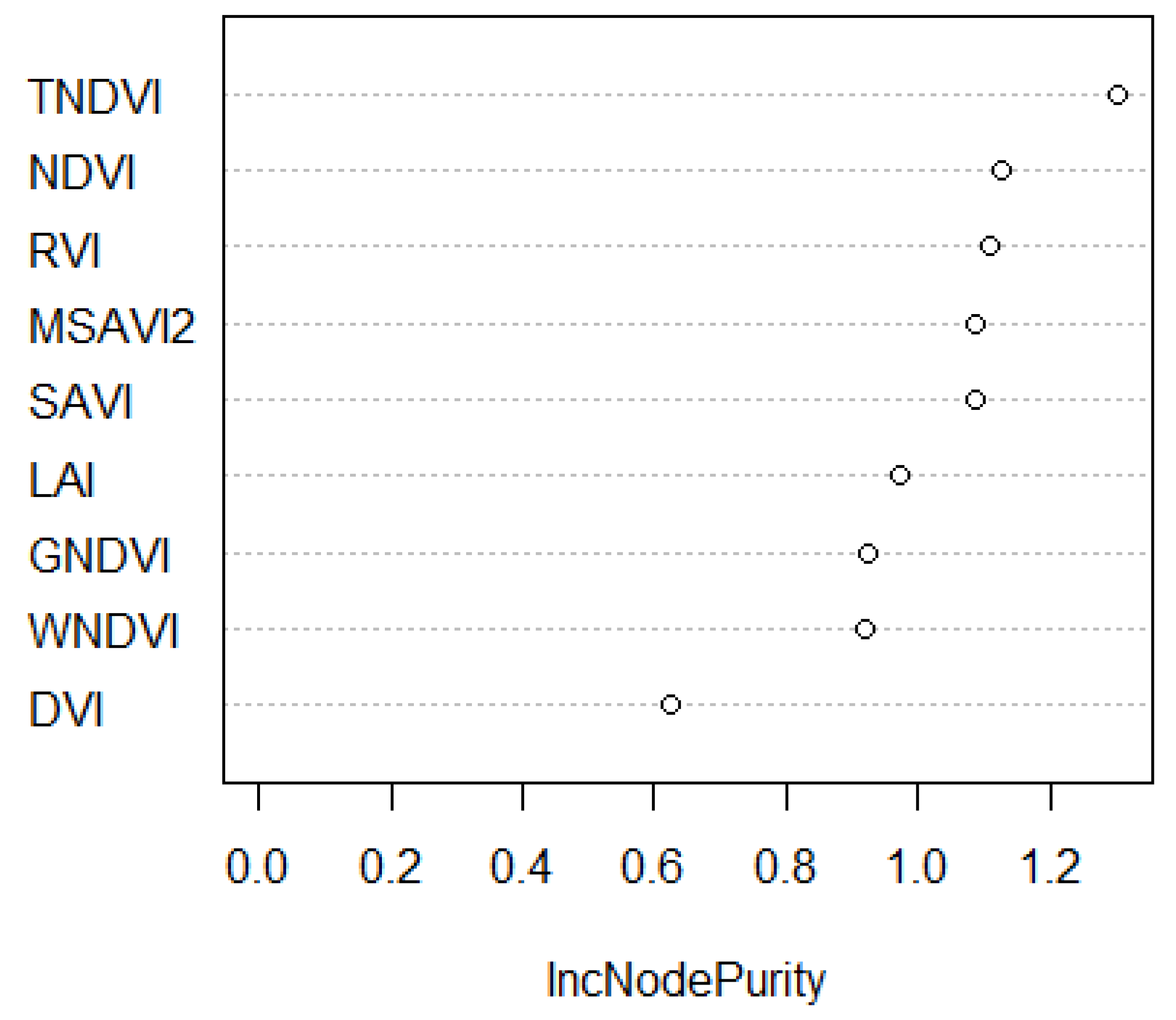
| Index | Equation | Reference | Description |
|---|---|---|---|
| Green Normalized Difference Vegetation Index (GNDVI) | [68] | More sensitive than NDVI to identifying different concentration rates of chlorophyll. | |
| Normalized Difference Vegetation Index (NDVI) | [69] | Has the capacity for assessing regional and global vegetation fluctuations. It is more sensitive to reflectance from soil background and tends to saturate for high biomass canopies. | |
| Soil Adjusted Vegetation Index (SAVI) | [70] | Used to correct NDVI for the influence of soil brightness in areas with low vegetative cover. | |
| Modified Soil Adjusted Vegetation Index 2 (MSAVI2) | [71] | Does not rely on a soil line principle and has a simpler algorithm. It is mainly applied in plant growth analysis. | |
| Ratio Vegetation Index (RVI) | [72] | Sensitive to green vegetation and is highly correlated with LAI and leaf biomass. | |
| Difference Vegetation Index (DVI) | [69] | Very sensitive to the amount of vegetation and changes in the soil background. | |
| Transformed Normalized Difference Vegetation Index (TNDVI) | [73] | Indicates a better correlation between the amount of green biomass that is found in a pixel. | |
| Weighted Difference Vegetation Index (WDVI) | [74] | Very sensitive to atmospheric variations and has a correction factor on the slope of the soil line. |
| Site 1 | Site 2 | |
|---|---|---|
| Variable | R2 | R2 |
| LAI | 0.45 | 0.70 |
| GNDVI | 0.21 | 0.70 |
| NDVI | 0.26 | 0.65 |
| SAVI | 0.26 | 0.79 |
| DVI | 0.26 | 0.56 |
| MSAVI2 | 0.25 | 0.69 |
| RVI | 0.27 | 0.73 |
| TNDVI | 0.26 | 0.59 |
| WNDVI | 0.27 | 0.89 |
| Variables | Model | R2 | RMSE | p-Value |
|---|---|---|---|---|
| All variables | RF All | 0.35 | 1.23 | 0.22 |
| TNDVI, NDVI, RVI, MSAVI2, and SAVI | RF5 | 0.82 | 1.00 | 0.01 ** |
| TNDVI, NDVI, and RVI | MLR | 0.98 | 0.18 | 0.02 ** |
| Variables | Method | R2 | RMSE | p-Value |
|---|---|---|---|---|
| TNDVI, NDVI, RVI, MSAVI2, and SAVI | RF5 | 0.96 | 0.29 | 0.001 ** |
| TNDVI, NDVI, and RVI | MLR | 0.84 | 0.84 | 0.02 ** |
| Date | Growth Stage | Model | R2 | RMSE (kg/ha) | p-Value |
|---|---|---|---|---|---|
| 7 March 2020 | R3/beginning pod stage | MLR | 0.57 | 0.99 | 0.08 |
| RF5 | 0.59 | 0.97 | 0.070 | ||
| 31 March 2020 | R5/beginning seed stage | MLR | 0.70 | 0.66 | 0.370 |
| RF5 | 0.95 | 0.35 | 0.001 ** |
| Farm | Reported Yield (kg/ha) | Predicted Yield (kg/ha) | Difference (kg/ha) | % Difference |
|---|---|---|---|---|
| Farm A | 3180.72 | 3226.46 | −45.74 | −1.44 |
| Farm B | 1180.33 | 1190.31 | −9.98 | −0.85 |
| Farm C | 2400.56 | 2461.79 | −61.23 | −2.55 |
| Farm D | 140.75 | 156.88 | −16.13 | −11.46 |
Publisher’s Note: MDPI stays neutral with regard to jurisdictional claims in published maps and institutional affiliations. |
© 2022 by the authors. Licensee MDPI, Basel, Switzerland. This article is an open access article distributed under the terms and conditions of the Creative Commons Attribution (CC BY) license (https://creativecommons.org/licenses/by/4.0/).
Share and Cite
Kpienbaareh, D.; Mohammed, K.; Luginaah, I.; Wang, J.; Bezner Kerr, R.; Lupafya, E.; Dakishoni, L. Estimating Groundnut Yield in Smallholder Agriculture Systems Using PlanetScope Data. Land 2022, 11, 1752. https://doi.org/10.3390/land11101752
Kpienbaareh D, Mohammed K, Luginaah I, Wang J, Bezner Kerr R, Lupafya E, Dakishoni L. Estimating Groundnut Yield in Smallholder Agriculture Systems Using PlanetScope Data. Land. 2022; 11(10):1752. https://doi.org/10.3390/land11101752
Chicago/Turabian StyleKpienbaareh, Daniel, Kamaldeen Mohammed, Isaac Luginaah, Jinfei Wang, Rachel Bezner Kerr, Esther Lupafya, and Laifolo Dakishoni. 2022. "Estimating Groundnut Yield in Smallholder Agriculture Systems Using PlanetScope Data" Land 11, no. 10: 1752. https://doi.org/10.3390/land11101752