A Protected Area Connectivity Evaluation and Strategy Development Framework for Post-2020 Biodiversity Conservation

Abstract

Maintaining and improving the connectivity of protected areas (PAs) is essential for biodiversity conservation. The Post-2020 Global Biodiversity Framework (GBF) aims to expand the coverage of well-connected PAs and other effective area-based conservation measures to 30% by 2030. We proposed a framework to evaluate the connectivity of PAs and developed strategies to maintain and improve the connectivity of PAs based on PA connectivity indicators, and we applied this framework to China’s terrestrial PAs. We considered that the concept of PA connectivity is at the level of both PA patches and PA networks, including four aspects: intra-patch connectivity, inter-patch connectivity, network connectivity, and PA–landscape connectivity. We found that among China’s 2153 terrestrial PA patches, only 427 had good intra-patch connectivity, and their total area accounted for 11.28% of China’s land area. If inter-patch connectivity, network connectivity, and PA–landscape connectivity were taken as the criteria to evaluate PA connectivity, respectively, then the coverage of well-connected terrestrial PAs in China was only 4.07%, 8.30%, and 5.92%, respectively. Only seven PA patches have good connectivity of all four aspects, covering only 2.69% of China’s land. The intra-patch, inter-patch, network, and PA–landscape connectivity of China’s terrestrial PA network reached 93.41%, 35.40%, 58.43%, and 8.58%, respectively. These conclusions indicated that there is still a big gap between China’s PA connectivity and the Post-2020 GBF target, which urgently needs to be improved. We identified PA patches and PA networks of ecological zones that need to improve PA connectivity and identified improvement priorities for them. We also identified priority areas for connectivity restoration in existing PAs, potential ecological corridors between PAs, and priority areas for PA expansion to improve the connectivity of PAs in China. Application of our framework elsewhere should help governments and policymakers reach ambitious biodiversity conservation goals at national and global scales.

1. Introduction

Biodiversity loss and climate change are urgent and critical crises to which humanity must respond [1,2,3]. Connectivity can facilitate a range shift and the climate resilience of species [4,5]. Maintaining and improving connectivity is essential for achieving long-term biodiversity outcomes in response to climate change [6,7,8]. Research has shown that habitat connectivity is sensitive to climate change and may be lost more rapidly than habitat area [9,10]. In summary, connectivity loss has a robust, lasting, and negative impact on biodiversity and is, therefore, a major threat to biodiversity maintenance [11,12].

The establishment of protected areas (PAs) is a vital initiative for biodiversity conservation [13,14,15,16], and connectivity is necessary, and even of central importance, for the effectiveness of PAs [17,18]. Both the Conservation for Biodiversity Aichi Targets [19] and the Post-2020 Global Biodiversity Framework (GBF), which is under discussion globally, emphasize the importance of PA connectivity and set global PA connectivity targets. Aichi Targets and the First Draft of the Post-2020 GBF call for 17% and 30%, respectively, of the global land area to be conserved through well-connected PAs and other effective area-based conservation measures (OECMs) [19,20].

Research on connectivity evaluation has led to the development of different connectivity indicators [21,22]. The probability of connectivity (PC) is a widely used indicator to evaluate the connectivity of PAs [23,24,25]. Based on PC, Saura et al. (2018) used the ProtConn indicator and found that only 7.5% of global terrestrial land is covered by well-connected PAs, whereas in case of China, the value is 8–12% [26]. Ward et al. (2020) used the ConnIntact indicator and found that intact land structurally connected only 10% of the terrestrial PAs globally [27]. Among the existing global PA connectivity assessment studies, some focused on the connectivity of the PA network including intra-patch connectivity and inter-patch connectivity [25,26,28], while others concentrated on the connectivity between PA patches (inter-patch connectivity) [27,29]. It is necessary to integrate the connectivity at different levels and aspects into a unified framework to comprehensively describe connectivity and propose systematic approaches to address it accordingly.

We considered that the concept of PA connectivity includes the intra-patch connectivity, inter-patch connectivity, network connectivity, and PA–landscape connectivity of both PA patches and PA networks (Figure 1) based on previous studies [23,27,30,31,32]. For a PA network that includes several PA patches located in a landscape, we distinguish the above concepts of connectivity according to the following definition. The intra-patch connectivity of a PA patch means the connectivity within the PA patch. The inter-patch connectivity of a PA patch means the connectivity between it and other PA patches within the PA network. The network connectivity of a PA patch means its connectivity with the PA network that includes its intra-patch connectivity and its inter-patch connectivity with other PA patches. The PA–landscape connectivity of a PA patch means the connectivity between this PA patch and the whole landscape. The intra-patch connectivity of the PA network includes the connectivity within every PA patch of the PA network. The inter-patch connectivity of the PA network includes the connectivity between every patch pairs within the PA network. The network connectivity of the PA network includes the intra-patch connectivity of every PA patch within the PA network and the inter-patch connectivity between every patch pair within the PA network. The PA–landscape connectivity of the PA network includes the connectivity between every PA patch and the whole landscape.

This study proposed a set of indicators to evaluate the PA connectivity of both PA patches and PA networks based on dispersal probability and the PC indicator [23], and all of these indicators range from 0 to 1. The probability of connectivity of intra PA patches (PCintra) indicator measures intra-patch connectivity, the probability of connectivity of inter PA patches (PCinter) indicator measures inter-patch connectivity, the probability of connectivity with the PA network (PCnet) indicator measures network connectivity, and the probability of connectivity with the whole landscape (PCland) indicator measures PA–landscape connectivity. We established a PA connectivity evaluation and strategy development framework based on these PA connectivity indicators (Figure 1).

The aim of this study is to provide a framework on PA connectivity evaluation and improvement for post-2020 biodiversity conservation and illustrate how this framework can be applied and guide the management of PAs, using China as an example. In the methods section, we explain the calculation methods of different connectivity indictors and how to determine the connectivity maintenance or improvement strategies according to the connectivity evaluation results. In the results section, we show the calculation results of the connectivity indicators of the PA networks and PA patches in China, the connectivity strategy classification results of PAs based on connectivity indicators, and the spatial priority area to improve PA connectivity in China.

2. Materials and Methods

2.1. Protected Areas and Ecological Zones

The natural conservation geographical regionalization scheme of China [33], which aims to guide China’s biodiversity conservation and establishment of the PA system, was adopted in this study. This biogeographic regionalization scheme divides China’s land into 38 terrestrial ecological zones. The South China Sea island tropical humid zone (Ⅷ2), which has no terrestrial PAs, was not included in the analysis. This study assumed that PAs need to connect with PAs within the same ecological zone, and we evaluated PA connectivity separately at the ecological zone scale.

We used data collected for various types of terrestrial PAs in China, including 819 polygons and 3163 points. The polygon data included data for 10 national parks, which were mapped according to the national park pilot area plans released by the Chinese government. Data for 252 national nature reserves and 377 local nature reserves were extracted from information published by the Chinese government. The data were merged with data on 180 PAs in China provided by the World Database on Protected Areas (WDPA) for September 2020 (https://www.protectedplanet.net (accessed on 5 January 2021)). The point data included scenic areas, forest parks, and geoparks, which we collected according to information released by the Chinese government. Areas of high ecological integrity within 2 km of the point data were used instead of the point data, as many studies have shown that it is reasonable to use areas of high ecological integrity for connectivity analysis [30,34,35,36]. In this study, global-scale, very low human impact areas [37] and China-scale wilderness areas [38] were selected to form high ecological integrity areas. The polygon data were merged with the high ecological integrity areas that replaced the point data. We intersected the PA patches with ecological zones and obtained 2153 PA patches covering 14.68% of China’s land surface with a total area of 1,409,761 km².

2.2. Resistance Surface

The resistance surface measures how difficult it is for an organism or ecological flow to move successfully [36] or measures the relative cost of passing through a gridded mapped surface [39]. Many studies create resistance surfaces based on the degree of human modification, naturalness, or other similar indicators [30,39,40,41]. In this study, we created a resistance surface based on the global land-scale human modification indicator, HMc, which estimates the cumulative human modification of the land using 13 global human stressor datasets with 2016 as the median year; the value is between 0 and 1 and has a spatial resolution of 1 km [42]. The stressor datasets included human settlement (population density, built-up areas), agriculture (cropland, livestock), transportation (major roads, minor roads, two tracks, railroads), mining and energy production (mining, oil wells, wind turbines), and electrical infrastructure (powerlines, nighttime lights) [42]. Despite the uncertainties that global data might bring, this was the best available data on human modification of China’s land. We performed an exponential transformation of HMc, similar to Cao et al. (2020) [30], and we formed a resistance surface R between 1 and 1000 using the following equation:

$$\mathrm{R}=1+999\ast \frac{{\mathrm{e}}^{{\mathrm{HM}}_{\mathrm{c}}}-1}{\mathrm{e}-1}$$

(1)

Finally, we removed areas covered by water bodies and glaciers extracted from land use data of China from the resistance surface (Figure S1), assuming that terrestrial animals do not pass over glaciers or through water bodies during dispersal. The land use data were obtained from the Resources and Environmental Science Data Center, Chinese Academy of Sciences (Beijing, China; http://www.resdc.cn/ (accessed on 16 June 2021)).

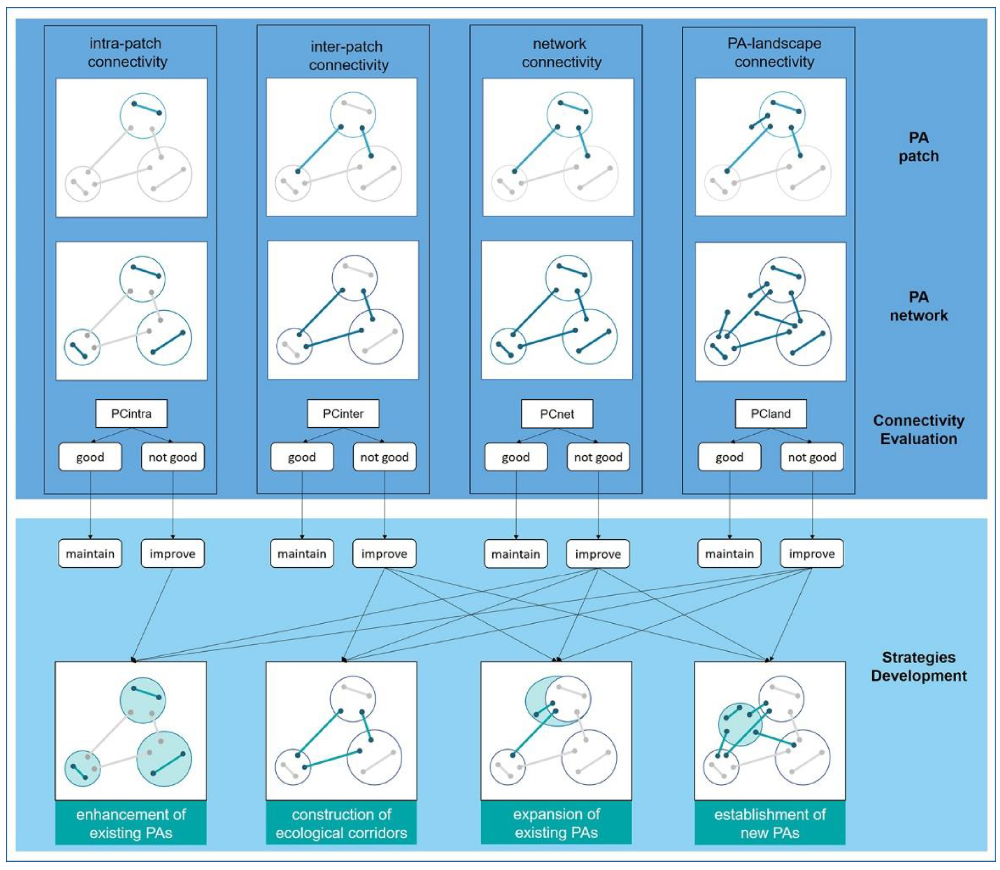
2.3. PA Connectivity Evaluation

For a PA network in a landscape that includes n PA patches, the area of PA patch i was noted as ${\mathrm{a}}_{\mathrm{i}}\left(\mathrm{i}=1,2\dots .,\mathrm{n}\right)$, the total area of the PA network was ${\mathrm{A}}_{\mathrm{N}}={\displaystyle \sum }_{\mathrm{i}=1}^{\mathrm{n}}{\mathrm{a}}_{\mathrm{i}}$, and the total area of the landscape was ${\mathrm{A}}_{\mathrm{L}}$. We evaluated the connectivity of PAs by dispersal probability, which can be estimated as a negative-exponential function of distance [32,43].

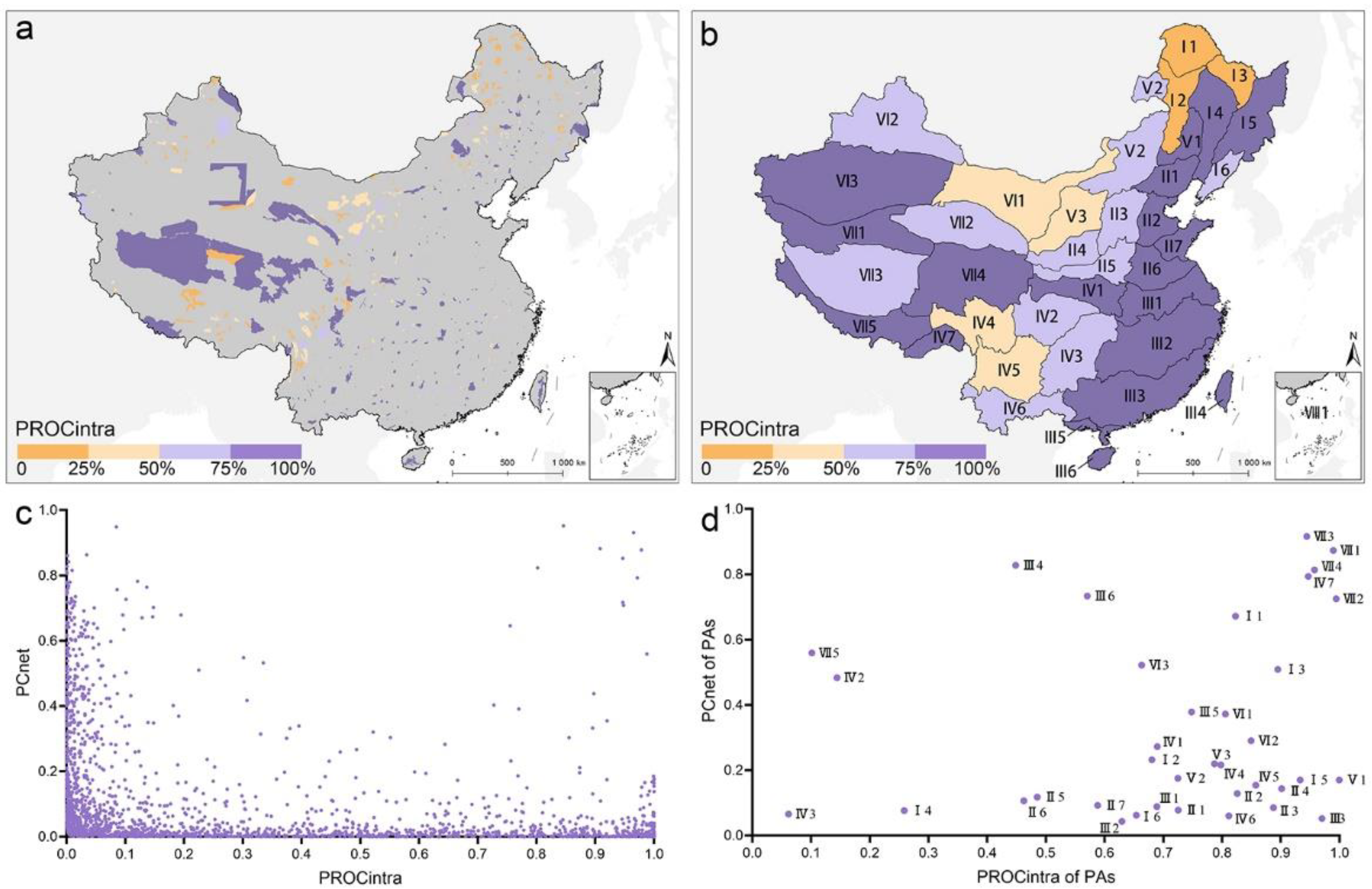
2.3.1. Intra-Patch Connectivity

As the distance an animal can disperse within a certain time duration is limited, the intra-patch connectivity of a patch can be simplified as the probability of a successful dispersal of a fixed distance from every point in a patch. We created a dispersal probability surface (with a value of P) (Figure S2) from the resistance surface. When the resistance surface is raster data with a cell side length D and a value R, for any cell on the raster surface, the cost distance is R when animal dispersal in the cell moves a distance D, and the dispersal probability P is as follows:

$$\mathrm{P}={\mathrm{e}}^{-\mathrm{h}\ast \mathrm{R}}$$

(2)

In the present study, R was between 1 and 1000, so we defined h as 1/1000, considering that the dispersal probability is 1/e (0.3679) when R takes the maximum possible value of 1000, and ${\mathrm{e}}^{-1/1000}$ (0.9990) when the resistance is the minimum value of 1, which is very close to 1.

The PCintra of PA patch i is defined as the probability of a successful dispersal of a fixed distance from any point within this patch and can be calculated as the average value of the dispersal probability surface within this patch:

$${\mathrm{PCintra}}_{\mathrm{i}}=\mathrm{average}\left(\mathrm{P}\right)\left(\mathrm{patch}\mathrm{i}\right)$$

(3)

The PCintra of the PA network is defined as the probability of a successful dispersal of a fixed distance from any point within patches can be calculated as the average value of the dispersal probability surface within the PA network:

$$\mathrm{PCintra}={{\displaystyle \sum }}_{\mathrm{i}=1}^{\mathrm{n}}\frac{{\mathrm{a}}_{\mathrm{i}}}{{\mathrm{A}}_{\mathrm{N}}}{ \ast \mathrm{PCintra}}_{\mathrm{i}}$$

(4)

After creating the dispersal probability surface, we used the partition statistics tool of ArcGIS 10.2 to calculate the PCintra of the PAs.

2.3.2. Inter-Patch Connectivity

Dispersal probability ${\mathrm{p}}_{\mathrm{ij}}$ characterizes the feasibility of a step between patches i and j, where a step is defined as a direct movement of a disperser between two habitat patches without passing by any other intermediate habitat patches [23]. We considered that an animal that moves from one patch i to another patch j first needs to move from some point A inside patch i to some point B on the edge of patch i; then, it moves successfully from point B through the matrix, to some point C on the edge of patch j, and from C to some point D inside patch j. The probability of successful dispersal from points A to B is ${\mathrm{PCintra}}_{\mathrm{i}}$, and the probability of successful dispersal from points B to C can be estimated as a negative-exponential function of the inter-patch distance ${\mathrm{d}}_{\mathrm{ij}}$ [32,43]. The probability of successful dispersal from points C to D is ${\mathrm{PCintra}}_{\mathrm{j}}$. Then, the probability of direct dispersal between patches i and j is calculated as follows (k is a constant):

$${\mathrm{p}}_{\mathrm{ij}}={\mathrm{PCintra}}_{\mathrm{i}}{ \ast \mathrm{e}}^{-{\mathrm{kd}}_{\mathrm{ij}}}{ \ast \mathrm{PCintra}}_{\mathrm{j}}$$

(5)

The value of ${\mathrm{p}}_{\mathrm{ij}}^{*}$ is the maximum product probability of all possible paths between patches i and j (including single-step paths) [23]. For the case of indirect dispersal from patch i through patch k to patch j, the probability is equal to the product of the probability of success of each step of the animal’s movement:

$${\mathrm{p}}_{\mathrm{ij}}^{\prime }={\mathrm{p}}_{\mathrm{i}}{ \ast \mathrm{e}}^{-{\mathrm{kd}}_{\mathrm{ik}}}{ \ast \mathrm{p}}_{\mathrm{k}}{\ast \mathrm{e}}^{-{\mathrm{kd}}_{\mathrm{kj}}}{\mathrm{p}}_{\mathrm{j}}$$

(6)

The inter-patch distance ${\mathrm{d}}_{\mathrm{ij}}$ can be estimated by the Euclidean distance or least-cost distance [23,44]. Measuring the connectivity between patches based on Euclidean distance does not reflect spatial heterogeneity, and this approach is considered unreasonable by some researchers [45]. Therefore, the least-cost distance was used as the inter-patch distance in this study. The Linkage Pathways Tool of Linkage Mapper Toolbox 2.0 (available at http://www.circuitscape.org/linkagemapper (accessed on 4 March 2021)) was used to calculate the least-cost distance between patches and obtain the least-cost paths (LCPs). The median distance refers to the distance corresponding to a dispersal probability of 0.5 and can be used to define the factor k in the equation for calculating the dispersal probability [25]. In the latest global PA network connectivity evaluation study, 10 km was used as the median distance [28]. Thus, we multiplied 10 km by the average value of the resistance surface of China (219.34) as the median cost distance, and then, we set k = 0.000316.

The ${\mathrm{PCinter}}_{\mathrm{I}}$ of PA patch i is defined as the probability that an animal randomly departs from any point within this patch and successfully disperses to any point in other patches, and it can be calculated as follows:

$${\mathrm{PCinter}}_{\mathrm{i}}=\frac{{{\displaystyle \sum }}_{\mathrm{j}\ne \mathrm{i}}^{\mathrm{n}}{\mathrm{a}}_{\mathrm{j}}{\mathrm{p}}_{\mathrm{ij}}^{*}}{{{\displaystyle \sum }}_{\mathrm{j}\ne \mathrm{i}}^{\mathrm{n}}{\mathrm{a}}_{\mathrm{j}}}=\frac{{{\displaystyle \sum }}_{\mathrm{j}\ne \mathrm{i}}^{\mathrm{n}}{\mathrm{a}}_{\mathrm{j}}{\mathrm{p}}_{\mathrm{ij}}^{*}}{{\mathrm{A}}_{\mathrm{N}}-{\mathrm{a}}_{\mathrm{i}}}$$

(7)

The $\mathrm{PCinter}$ of the PA network is defined as the probability that an animal randomly departs from any point within the network and successfully disperses to any point located in different patches from the departure point. The probability that the departure point falls in patch i is ${\mathrm{a}}_{\mathrm{i}}/{\mathrm{A}}_{\mathrm{N}}\left(\mathrm{i}=1,2\dots .,\mathrm{n}\right)$; thus, the probability of successful dispersal is as follows:

$$\mathrm{PCinter}={{\displaystyle \sum }}_{\mathrm{i}=1}^{\mathrm{n}}\frac{{\mathrm{a}}_{\mathrm{i}}}{{\mathrm{A}}_{\mathrm{N}}}{ \ast \mathrm{PCinter}}_{\mathrm{i}}$$

(8)

After calculating PCintra for each PA patch and ${\mathrm{d}}_{\mathrm{ij}}$ between patches, we calculated the PCinter of each PA patch using the Conefor 2.6 software [46].

2.3.3. Network Connectivity

The ${\mathrm{PCnet}}_{\mathrm{i}}$ of patch i is defined as the probability that an animal randomly departs from any point within this patch and successfully disperses to any point in the network. The probability that the destination point falls in patch j is ${\mathrm{a}}_{\mathrm{j}}/{\mathrm{A}}_{\mathrm{N}}\left(\mathrm{j}=1,2\dots .,\mathrm{n}\right)$; thus, the probability of successful dispersal of an animal from patch i can be calculated as follows:

$${\mathrm{PCnet}}_{\mathrm{i}}=\frac{{{\displaystyle \sum }}_{\mathrm{j}=1}^{\mathrm{n}}{\mathrm{a}}_{\mathrm{j}}{\mathrm{p}}_{\mathrm{ij}}^{*}}{{\mathrm{A}}_{\mathrm{N}}}={\mathrm{PCintra}}_{\mathrm{i}}\ast \frac{{\mathrm{a}}_{\mathrm{i}}}{{\mathrm{A}}_{\mathrm{N}}}+{\mathrm{PCinter}}_{\mathrm{i}}\ast \frac{{\mathrm{A}}_{\mathrm{N}}-{\mathrm{a}}_{\mathrm{i}}}{{\mathrm{A}}_{\mathrm{N}}}$$

(9)

The PCnet of the PA network is defined as the probability that an animal randomly departs from any point in the network and successfully disperses to any point in the network. The probability that the departure point falls in patch i is ${\mathrm{a}}_{\mathrm{i}}/{\mathrm{A}}_{\mathrm{N}}\left(\mathrm{i}=1,2\dots .,\mathrm{n}\right)$; thus, the probability of successful dispersal was calculated as follows:

$$\mathrm{PCnet}={{\displaystyle \sum }}_{\mathrm{i}=1}^{\mathrm{n}}\frac{{\mathrm{a}}_{\mathrm{i}}}{{\mathrm{A}}_{\mathrm{N}}}{\ast \mathrm{PCnet}}_{\mathrm{i}}$$

(10)

The proportion of connectivity of intra PA patches (PROCintra) indicator and the proportion of connectivity of inter PA patches (PROCinter) indicator describe the proportion of network connectivity provided by intra-patch connectivity and inter-patch connectivity, respectively.

The ${\mathrm{PROCintra}}_{\mathrm{i}}$ and ${\mathrm{PROCinter}}_{\mathrm{i}}$ of patch i can be calculated as follows:

$${\mathrm{PROCintra}}_{\mathrm{i}}=\frac{{\mathrm{a}}_{\mathrm{i}}{\mathrm{p}}_{\mathrm{ii}}^{*}}{{{\displaystyle \sum }}_{\mathrm{j}=1}^{\mathrm{n}}{\mathrm{a}}_{\mathrm{j}}{\mathrm{p}}_{\mathrm{ij}}^{*}}$$

(11)

$${\mathrm{PROCinter}}_{\mathrm{i}}=\frac{{{\displaystyle \sum }}_{\mathrm{j}=1,\mathrm{j}\ne \mathrm{i}}^{\mathrm{n}}{\mathrm{a}}_{\mathrm{j}}{\mathrm{p}}_{\mathrm{ij}}^{*}}{{{\displaystyle \sum }}_{\mathrm{j}=1}^{\mathrm{n}}{\mathrm{a}}_{\mathrm{j}}{\mathrm{p}}_{\mathrm{ij}}^{*}}=1-{\mathrm{PROCintra}}_{\mathrm{i}}$$

(12)

The PROCintra and PROCinter of the PA network can be calculated as follows:

$$\mathrm{PROCintra}=\frac{{{\displaystyle \sum }}_{\mathrm{i}=1}^{\mathrm{n}}{\mathrm{a}}_{\mathrm{i}}{ \ast \mathrm{PCnet}}_{\mathrm{i}}{ \ast \mathrm{PROCintra}}_{\mathrm{i}}}{{{\displaystyle \sum }}_{\mathrm{i}=1}^{\mathrm{n}}{\mathrm{a}}_{\mathrm{i}}{ \ast \mathrm{PCnet}}_{\mathrm{i}}}$$

(13)

$$\mathrm{PROCinter}=\frac{{{\displaystyle \sum }}_{\mathrm{i}=1}^{\mathrm{n}}{\mathrm{a}}_{\mathrm{i}}{ \ast \mathrm{PCnet}}_{\mathrm{i}}{ \ast \mathrm{PROCinter}}_{\mathrm{i}}}{{{\displaystyle \sum }}_{\mathrm{i}=1}^{\mathrm{n}}{\mathrm{a}}_{\mathrm{i}}{ \ast \mathrm{PCnet}}_{\mathrm{i}}}=1-\mathrm{PROCintra}$$

(14)

2.3.4. PA–Landscape Connectivity

The ${\mathrm{PCland}}_{\mathrm{I}}$ of patch i is defined as the probability that an animal randomly departs from any point within this patch and successfully disperses to any point in the landscape. In this study, we assumed that when the destination point is out of the PA patches, the animal could not disperse successfully. The probability that the destination point falls in patch j is ${\mathrm{a}}_{\mathrm{j}}/{\mathrm{A}}_{\mathrm{L}}\left(\mathrm{j}=1,2\dots .,\mathrm{n}\right)$; thus, the probability of successful dispersal of an animal from patch i can be calculated as follows:

$${\mathrm{PCland}}_{\mathrm{i}}=\frac{{{\displaystyle \sum }}_{\mathrm{j}=1}^{\mathrm{n}}{\mathrm{a}}_{\mathrm{j}}{\mathrm{p}}_{\mathrm{ij}}^{*}}{{\mathrm{A}}_{\mathrm{L}}}={\mathrm{PCnet}}_{\mathrm{i}}\ast \frac{{\mathrm{A}}_{\mathrm{N}}}{{\mathrm{A}}_{\mathrm{L}}}$$

(15)

The PCland of the PA network is defined as the probability that an animal randomly departs from any point in the PA network and successfully disperses to any point in the landscape. The probability that the destination point falls in patch i is ${\mathrm{a}}_{\mathrm{i}}/{\mathrm{A}}_{\mathrm{L}}\left(\mathrm{i}=1,2\dots .,\mathrm{n}\right)$; thus, the probability of successful dispersal was calculated as follows:

$$\mathrm{PCland}={{\displaystyle \sum }}_{\mathrm{i}=1}^{\mathrm{n}}\frac{{\mathrm{a}}_{\mathrm{i}}}{{\mathrm{A}}_{\mathrm{N}}}{ \ast \mathrm{PCland}}_{\mathrm{i}}=\mathrm{PCnet} \ast \frac{{\mathrm{A}}_{\mathrm{N}}}{{\mathrm{A}}_{\mathrm{L}}}$$

(16)

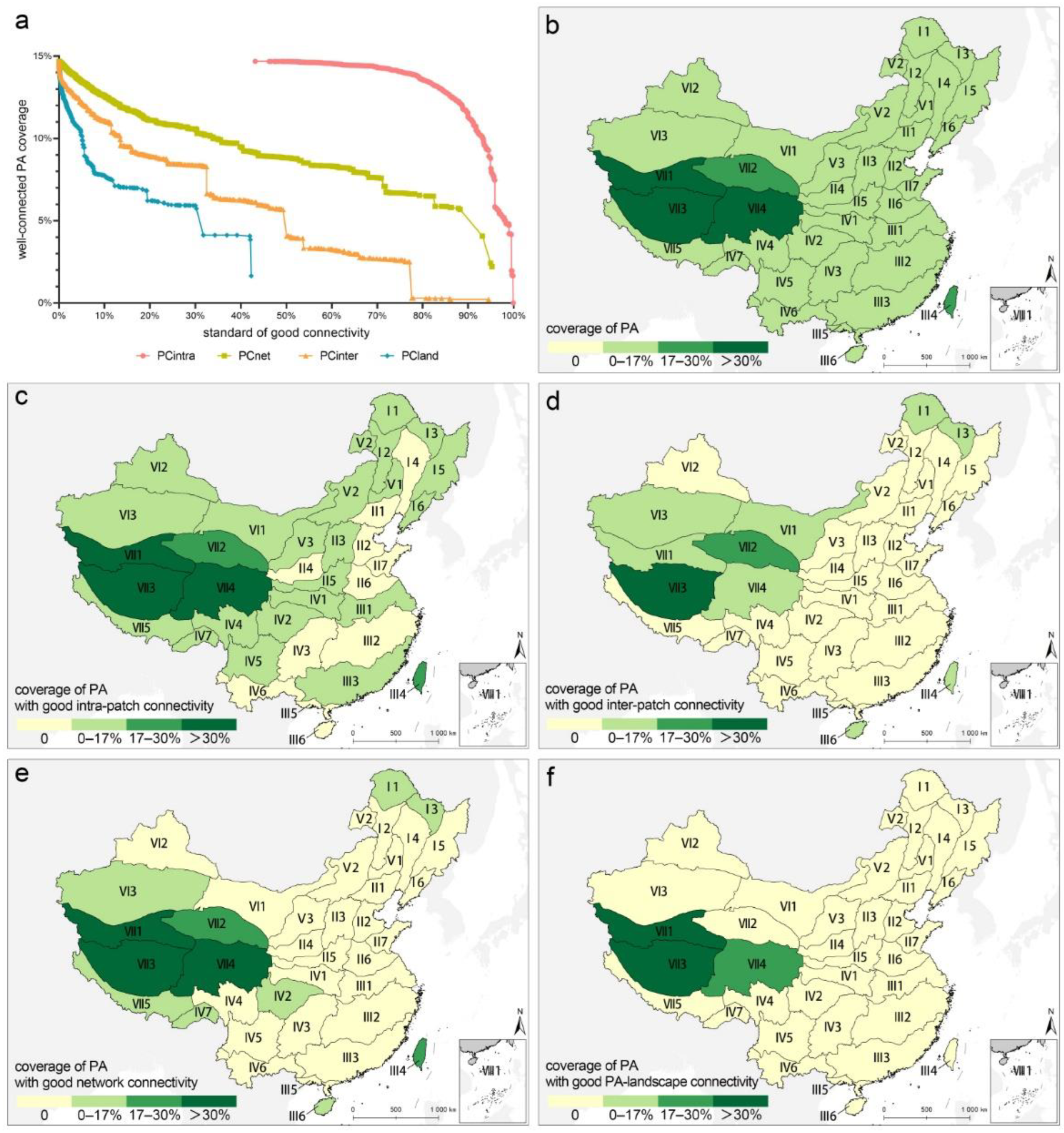
2.3.5. PAs with Good Connectivity

According to the Post-2020 GBF objectives for PAs, it is necessary to define good connectivity. For PA patches and PA networks, when the PCland indicator reaches 30%, its PA–landscape connectivity is considered to be well; otherwise, its PA–landscape connectivity is not well based on the Post-2020 GBF. Similarly, we considered whether the PCintra, PCinter, and PCnet reach 90%, 50%, and 60% as the standards to judge whether the intra-patch connectivity, inter-patch connectivity, and network connectivity are good. There is a relative lack of research on the standards of good connectivity. There are two main reasons why we decided on these standards. First, these indicators have a relative size relationship; that is, for a PA patch, the value of PCintra is greater than the value of PCnet, and the value of PCnet is greater than the value of PCinter, so they should be given different standards. Second, 90%, 50%, and 60% are values that are easier for managers of PAs to understand. We discussed the impact of standards on the coverage of well-connected PAs in the discussion section.

2.4. Strategy Development for PA Connectivity

2.4.1. Strategy Classification of PA Connectivity Based on Indicators

We classified PA patches and PA networks into 16 categories based on whether the four aspects of connectivity were good or not, and each category corresponded to a four-letter string, although some may not actually exist. When a PA patch’s intra connectivity was good, it was marked as category A; otherwise, it was marked as category B. We classified inter-patch connectivity, network connectivity and PA–landscape connectivity in the same way. We combined those letters in order of intra, inter, network and PA–landscape to obtain a four-letter string. For example, PAs classified as AAAA had good intra-patch, inter-patch, network and PA–landscape connectivity, and class ABBB only had good intra-patch connectivity.

When the intra-patch, inter-patch, network or PA–landscape connectivity reaches good, it should be maintained, and when it is not good, it should be improved. For example, PAs classified as AAAA needed to maintain the four aspects of connectivity, and class AAAB needed to maintain intra-patch, inter-patch and network connectivity and improve PA–landscape connectivity.

There are four strategies to improve PA connectivity (Figure 1). The enhancement of existing PAs through habitat restoration, construction of wildlife crossings, and other methods is a strategy to improve the intra-patch connectivity, which then can improve inter-patch, network and PA–landscape connectivity. The construction of ecological corridors is a widely used effective measure to improve inter-patch connectivity [7,47,48], which then can improve network and PA–landscape connectivity. Similar to ecological corridors, the expansion of existing PAs and the establishment of new PAs can reduce the cost distance between existing PA patches and thus improve inter-patch, network and PA–landscape connectivity. These two methods can also improve PA–landscape connectivity by increasing PA coverage.

2.4.2. Spatial Priority Area for PA Connectivity Improvement

Within existing PA patches requiring improved intra-patch connectivity, areas with a dispersal probability of less than 90% (corresponding to the good intra-patch connectivity standard) were identified as priority areas for enhancing existing PAs. We identified the LCPs between two PA patches that both needed to improve inter-patch connectivity as priority ecological corridors. We considered high ecological integrity areas along these LCPs as priority areas for the expansion of existing PAs and the establishment of new PAs because of both high integrity and high connectivity contribution.

3. Results

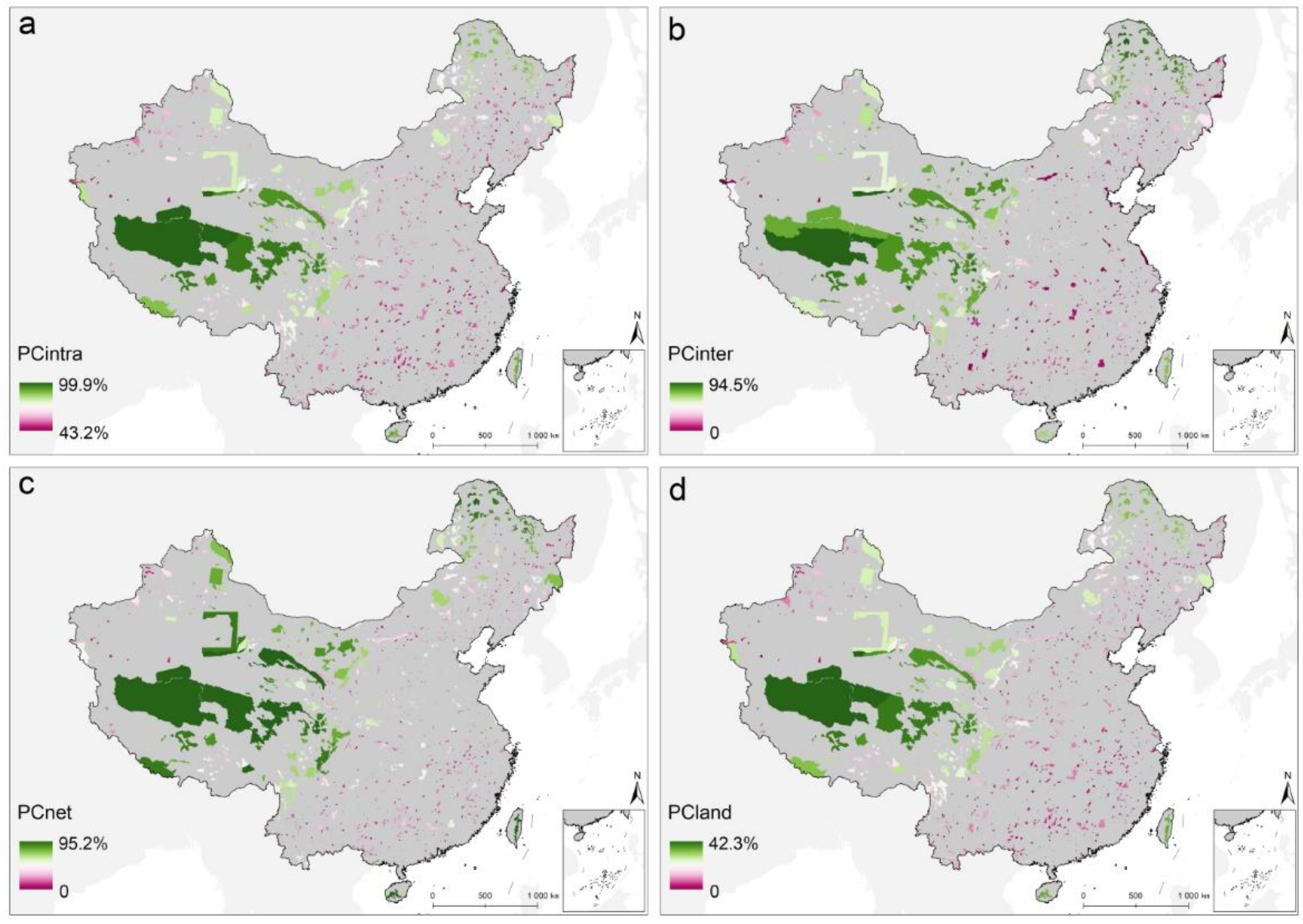
3.1. Connectivity of PAs in China

Our result showed that the PCintra of China’s PA network was 93.41%, which indicated that the connectivity within China’s PA network is good. However, the PCintra of the 2153 PA patches varied greatly from 99.90% to 43.17% (Figure 2a). A total of 427 patches had good intra-patch connectivity, accounting for 11.28% of China’s land area. The intra-patch connectivity of the PA network was not good in 22 of the 37 ecological zones (

Table 1. Connectivity indicators of ecological zones’ PA network.

No.	Ecological Zone	PCintra of PAs (%)	PCinter of PAs (%)	PCnet of PAs (%)	PCland of PAs (%)
Ⅰ1	Northern Daxing’anling cold-temperate semi-humid zone	96.33	65.06	67.17	10.18
Ⅰ2	Southern Daxing’anling temperate semi-humid zone	92.11	20.59	23.16	3.32
Ⅰ3	Xiaoxing’anling temperate semi-humid zone	91.28	49.57	50.87	8.63
Ⅰ4	Northeast Plain temperate semi-humid zone	74.44	1.52	7.62	0.38
Ⅰ5	Changbai Mountain temperate humid semi-humid zone	84.97	3.98	17.01	2.57
Ⅰ6	Liaodong Peninsula warm-temperate semi-humid zone	77.20	2.21	6.20	0.31
Ⅱ1	Yanshan Mountain warm-temperate semi-humid zone	77.64	1.26	7.78	0.36
Ⅱ2	Haihe Plain warm-temperate semi-humid zone	59.36	0.09	12.87	0.33
Ⅱ3	Shanxi Plateau warm-temperate semi-humid zone	82.92	2.51	8.48	0.24
Ⅱ4	Northern Shaanxi and Longzhong Plateau warm-temperate semi-arid zone	81.11	4.07	14.31	0.41
Ⅱ5	Southern Taihang and northern Qinling warm-temperate semi-humid zone	78.71	5.64	11.75	0.48
Ⅱ6	Yellow and Huai River Plain warm-temperate semi-humid zone	55.20	0.01	10.60	0.29
Ⅱ7	Shandong Peninsula warm-temperate semi-humid zone	64.65	0.10	9.22	0.16
Ⅲ1	Middle and lower reaches of Yangtze River northern subtropical humid zone	69.97	0.49	8.84	0.38
Ⅲ2	Middle and lower reaches of Yangtze River central subtropical humid zone	79.52	0.84	4.28	0.19
Ⅲ3	Southeast China humid south subtropical zone	80.57	0.78	5.18	0.20
Ⅲ4	Taiwan Island tropical subtropical humid zone	92.02	23.89	82.76	16.27
Ⅲ5	Southeast China tropical humid zone	82.20	1.90	37.81	1.01
Ⅲ6	Hainan Island tropical humid zone	84.57	21.78	73.35	12.19
Ⅳ1	Qinba Mountains northern subtropical humid zone	88.27	7.23	27.21	3.92
Ⅳ2	Sichuan basin and marginal mountains subtropical humid zone	88.25	30.58	48.33	5.68
Ⅳ3	Guizhou plateau and marginal mountains subtropical humid zone	79.79	2.57	6.56	0.24
Ⅳ4	Northern Transverse Mountains subtropical humid semi-humid zone	93.23	12.59	21.61	3.36
Ⅳ5	Southern Transverse Mountains central subtropical humid zone	81.58	9.18	15.38	1.60
Ⅳ6	Southwest China tropical subtropical humid zone	81.61	2.00	6.00	0.36
Ⅳ7	Eastern edge of the Himalayas tropical humid zone	93.56	33.41	79.35	6.59
Ⅴ1	Xiliaohe River temperate semi-arid zone	81.07	4.50	16.99	1.48
Ⅴ2	Eastern Inner Mongolia Plateau temperate semi-arid zone	90.28	6.20	17.50	2.78
Ⅴ3	Ordos Plateau and surrounding mountains temperate semi-arid zone	83.97	14.15	21.96	2.42
Ⅵ1	Western Inner Mongolia Plateau temperate arid zone	95.22	31.23	37.19	5.25
Ⅵ2	Northern Xinjiang temperate arid semi-arid zone	92.79	12.29	29.03	3.79
Ⅵ3	Southern Xinjiang temperate warm temperate arid zone	97.65	10.85	52.16	4.11
Ⅶ1	Kunlun Mountains alpine arid zone	99.68	32.30	87.34	39.65
Ⅶ2	Qaidam and Qilian Mountains alpine arid semi-arid zone	94.84	51.87	72.50	17.02
Ⅶ3	Qiangtang Plateau alpine arid zone	99.02	76.71	91.59	40.50
Ⅶ4	East Tibet and south Qinghai alpine semi-humid zone	95.20	48.74	81.37	27.88
Ⅶ5	Southern Tibetan alpine semi-humid semi-arid zone	93.29	13.45	55.92	9.17
Ⅷ1	South China Sea islands tropical humid zone	—	—	—	—

).

The PCinter of China’s PA network was 35.40%, which was not good. The PCinter of the PA patches varied from 94.50% to 0 (Figure 2b). A total of 116 patches had good inter-patch connectivity, accounting for 4.07% of China’s land area. Only three ecological zones’ PA network had good inter-patch connectivity (Table 1), including the Northern Daxing’anling cold-temperate semi-humid zone, the Qaidam and Qilian Mountains alpine arid semi-arid zone and the Qiangtang Plateau alpine arid zone (Ecological Zones Ⅰ1, Ⅶ2 and Ⅶ3).

The PCnet of China’s PA network was 58.43% and very close to good. The PCnet of the PA patches varied from 95.21% to 0 (Figure 2c). Only 90 PA patches had good network connectivity, accounting for 8.30% of China’s land area. Eight ecological zones had good network connectivity (Table 1).

The PCland of China′s PA network was 8.58%, which was not good. The PCland of the PA patches varied from 42.28% to 0 (Figure 2d). Only nine PA patches had good inter-patch connectivity, accounting for 5.92% of China’s land area. Two ecological zones on the Qinghai-Tibet Plateau have good PA–landscape connectivity (Table 1), including the Qiangtang Plateau alpine arid zone and the Kunlun Mountains alpine arid zone (Ecological Zones Ⅶ1 and Ⅶ3).

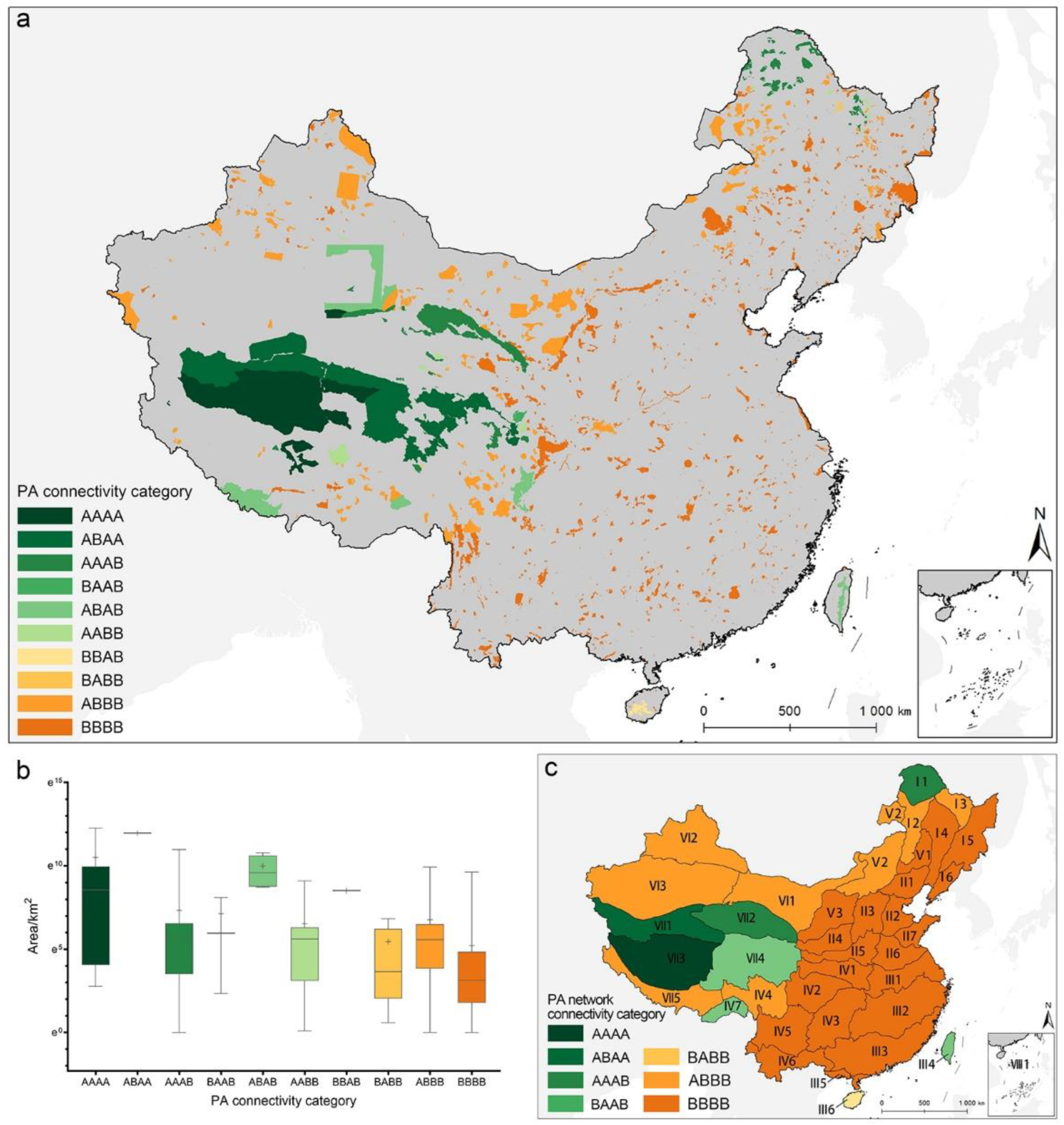
3.2. PA Connectivity Strategy Classification

Only seven PA patches located in Ecological Zones Ⅶ1 and Ⅶ4 were classified as AAAA, accounting for 2.67% of China’s land area (Figure 3a). Two PA patches were classified as ABAA and also located in Ecological Zones Ⅶ1 and Ⅶ4, accounting for 3.26% of China’s land area. A total of 72 PA patches were classified as AAAB, accounting for 1.16% of China’s land area. These PA patches had good network connectivity and need to be extended or have new PAs established around them to improve their PA–landscape connectivity. Only 3, 5, 26, and 1 PA patches are classified as BAAB, ABAB, AABB, and BBAB, respectively. A total of 315 PA patches were classified as ABBB, accounting for 2.89% of China’s land area. A total of 1714 PA patches were classified as BBBB, accounting for 2.89% of China’s land area. These PA patches urgently needed to be improved in all aspects of connectivity. The connectivity of large PA patches was not necessarily good, and in fact, many large PA patches were classified as ABBB or BBBB (Figure 3b).

Among the ecological zones, only the PA network of the Qiangtang Plateau alpine arid zone (Ecological Zone Ⅶ3) was classified as AAAA. Ecological Zone Ⅶ1 was classified as ABAA and should focus on improving inter-patch connectivity. Ecological Zones Ⅰ1 and Ⅶ2 were classified as AAAB and should focus on improving PA–landscape connectivity by increasing PA coverage. Ecological Zones Ⅲ4, Ⅳ7 and Ⅶ4 were classified as ABAB; this suggested that they should improve both inter-patch connectivity and PA–landscape connectivity. Ecological Zone Ⅲ6 was classified as BBAB. Ecological Zones Ⅰ2, Ⅰ3, Ⅳ4, Ⅴ2, Ⅵ1, Ⅵ2, Ⅵ3, and Ⅶ5 were classified as ABBB. The other 21 ecological zones were classified as BBBB and should urgently improve PA connectivity in multiple ways.

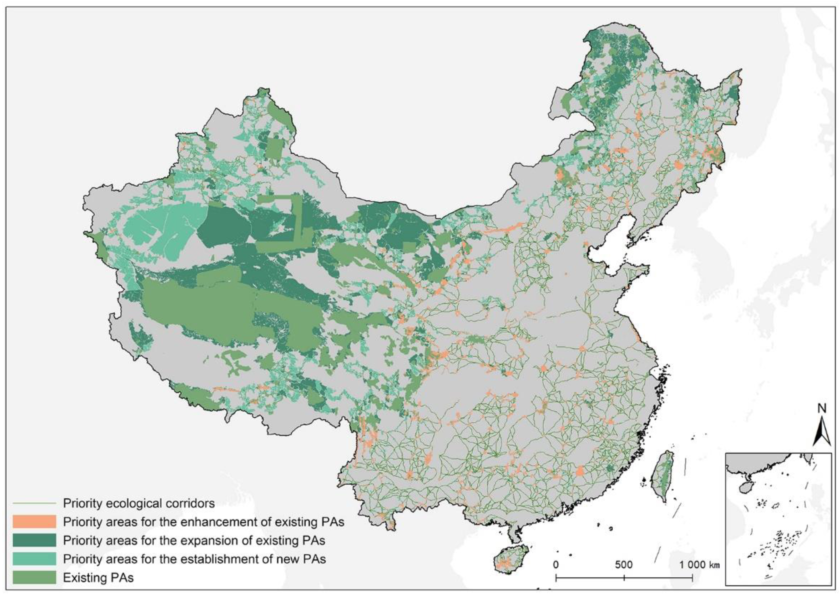
3.3. Spatial Priority Area to Improve PA Connectivity in China

A total of 17.24% of the area of existing PAs (243,060 km²) were priority areas for connectivity enhancement to improve intra-patch connectivity (Figure 4). We identified 4344 potential priority ecological corridors between PAs (Figure 4). The priority area for expanding existing PAs included 1253 patches with a total area of 1,123,240 km², covering 11.70% of China’s land area (Figure 4). The priority area for establishing new PAs included 9284 patches with a total area of 712,087 km², covering 7.41% of China’s land area (Figure 4).

4. Discussion

4.1. Importance of Intra-Patch Connectivity

We suggested that the intra-patch connectivity should be regarded as important in both the evaluation and the improvement of PA connectivity. Some connectivity evaluation studies consider only inter-patch connectivity, ignoring the contribution of intra-patch connectivity to the overall connectivity, which can lead to erroneous conclusions in connectivity evaluations [31]. We calculated the PROCintra of China’s PA network as 74.69%, which indicated that intra-patch connectivity contributed much more to network connectivity than inter-patch connectivity in China. The PROCintra values of 467 PA patches were higher than 75% and the PROCintra values of 213 patches were between 75% and 50% (Figure 5a). The PROCintra values of the PA network of 30 ecological zones were higher than the PROCinter values (Figure 5b). We also found that there was no significant correlation between the value of PCintra indicator and PCnet for both PA patches and PA networks (Figure 5c,d). This indicated that the relationships between intra-patch, inter-patch, and network connectivity are complex.

Research on the connectivity performance of PA management is lacking, leading to the assumption that PAs are effectively managed for connectivity in many studies [26]. Previous studies have generally assumed an excellent intra-patch connectivity (as a value of 1) [28,44]. We found that such assumptions may significantly overestimate the network connectivity of PAs. We calculated the PCnet and PCland indicator of each ecological zone’s PA network assuming a PCintra of 1 for all PA patches (Table S1). Under this assumption, the PCnet of China would increase from 58.43% to 62.11%, and the Pcnet of Xiaoxing’anling temperate semi-humid zone (Ecological Zone Ⅰ3) would increase from 50.87% to 71.07%. Clearly, overvalued network connectivity is not conducive to developing targeted enhancement strategies.

Improving intra-patch connectivity may effectively improve the connectivity of the PA network. For example, our findings showed that the Yellow and Huai River Plain warm-temperate semi-humid zone (Ecological Zone Ⅱ6) had the poorest intra-patch connectivity of PAs in the ecological zones of China. If the PCintra of the PAs of this ecological zone is improved from 55.20% to 1, then the PCnet would improve from 10.60% to 19.44%. This result was consistent with previous studies suggesting that the connectivity within core areas is important [31]. This suggested that decision makers of PAs with similar circumstances should first begin to improve connectivity within PAs to ensure a high-quality PA system.

4.2. Evaluation of Connectivity at the Patch Scale

In the previous network connectivity analysis of PAs, some studies have discussed the contribution of patches to the connectivity of a PA network [44,49,50]. In addition, others have focused on mapping potential inter-patch dispersal routes [51]. The mapping studies have identified areas that are important as potential dispersal routes by applying concepts such as current density and betweenness centrality [40,52,53]. These studies have evaluated how well the PA network formed by the patches is connected, but they have not directly answered the question of how well connected the patches are. Therefore, the results might not directly guide managers in making decisions for PA patches.

Based on the dispersal probability between patches [43], we tried to extend the concept of PA connectivity from PA networks to PA patches. Our results showed that the connectivity strategy category of a PA network may be inconsistent with the connectivity strategy categories of PA patches within the network (Figure 3a,c). This indicated the need for connectivity evaluation at the patch scale.

Our PA connectivity evaluation framework for both PA patches and PA networks can support comparison and management decisions for the PA connectivity of countries, ecological zones, and administrative regions. Using our framework, the manager responsible for a PA can accurately assess the connectivity of the PA, apply a targeted approach to secure external funding and coordinate with managers of other PAs and external local governments. The manager of a region can clearly understand the connectivity of each PA in the region and how to enhance the connectivity of the regional PAs through coordination among the PAs.

4.3. Connectivity Indicators for Well-Connected PAs

It is important to identify connectivity’s own target with accompanying indicators to guide global conservation efforts [54]. The four indicators we propose can be used as a basis to evaluate whether the PAs are well-connected. The coverage of well-connected PAs in a region or country can then be calculated to compare with the post-2020 biodiversity conservation targets. In fact, the coverage of well-connected PAs depends on the coverage of PAs and the indicator standard of good connectivity (Figure 6a). Future research can further discuss which indicators to choose and how to determine the standard of good connectivity. We believed that the combined use of these indicators would contribute to a comprehensive understanding of PA connectivity.

The Post-2020 GBF requires 30% global land area coverage of well-connected PAs, and according to this requirement, among the 37 ecological zones, only Ecological Zones Ⅶ1, Ⅶ3 and Ⅶ4 had more than 30% PA coverage (Figure 6b). No matter which indicator was chosen as a criterion for good connectivity, only these three ecological zones may have over 30% coverage of well-connected PAs. Our results showed that 11 ecological zones did not have PA patches with good intra-patch connectivity, 27 ecological zones did not have PA patches with good inter-patch connectivity, 25 ecological zones did not have PA patches with good network connectivity and 34 ecological zones did not have PA patches with good PA–landscape connectivity (Figure 6c–f). Compared with the results of connectivity indicators of the PA network, the coverage of well-connected PAs more strongly indicated that the PA connectivity of these ecological zones urgently needs to be improved. We suggest that specifying which indicator or series of indicators to use in the Post 2020 GBF objectives is necessary to facilitate global awareness and begin initiatives to improve connectivity. At the same time, we recommend that countries consider using the series of indicators in our framework to describe PA connectivity to drive comprehensive conservation and enhancement measures at all levels.

4.4. Limitations and Future Research

First, uncertainties exist in the creation of the resistance surface. Both the selection of human modification data and the calculation method of transforming human modification data into resistance surface would bring uncertainty to the resistance surface. This has implications for the creation of dispersal probability surface and cost distances between PA patches based on resistance surfaces and thus creates uncertainties in the PA connectivity evaluation results. Many studies have discussed how to create resistance surfaces in connectivity research [30,39,53], but there is not a high degree of consensus among researchers on this question. Future research could focus on how to create resistance surfaces to evaluate PA connectivity.

Second, we did not consider the effect of PAs’ shape and area on intra-patch connectivity and led to uncertainty in the evaluation result of PAs’ intra-patch connectivity. A more reasonable evaluation method of intra-patch connectivity, such as the use of least-cost distance model or circuit model, is necessary in the future.

Third, the selection of median cost distance will bring uncertainty to the evaluation of connectivity between PAs. Some studies have analyzed the effect of median distance on inter-patch connectivity when using Euclidean distance to evaluate inter-patch connectivity [25,26], but scholars have not reached a high level of consensus on this issue. Future research should discuss how to determine the median cost distance when using least-cost distance to evaluate inter-patch connectivity.

5. Conclusions

In this study, we have proposed a unified framework to evaluate and develop strategies for PA connectivity, and the results can directly guide management decisions. This study proposed a conceptual framework for the connectivity of PAs that includes intra-patch, inter-patch, network and PA–landscape connectivity for both PA patches and PA networks, which can be evaluated logically and consistently in this framework. This framework provides a set of indicators for the post-2020 biodiversity conservation targets on well-connected PAs. The proposed framework considers the differences in the intra-patch connectivity of PAs and thus might provide a better evaluation of PAs’ inter-patch connectivity and network connectivity. The framework also includes how to develop strategies and identify priority areas to improve PA connectivity based on the evaluation results of PAs’ connectivity indicators. This study shows that the connectivity of China’s PAs is not good and needs to be improved. At the same time, the PA connectivity of the Qinghai-Tibet Plateau is relatively good, and attention should be paid to maintaining the connectivity of existing PAs in this region. The method proposed in this study can be used for the evaluation, improvement, and spatial planning of the connectivity of PAs at regional, national, and global scales. Our conceptual framework, indicators, and evaluation methods for connectivity can also be widely used in landscape connectivity research.

References

1. Díaz, S.; Fargione, J.; Chapin, F.S.; Tilman, D. Biodiversity Loss Threatens Human Well-Being. PLoS Biol. 2006, 4, e277. [Google Scholar] [CrossRef]
2. Patz, J.A.; Campbell-Lendrum, D.; Holloway, T.; Foley, J.A. Impact of Regional Climate Change on Human Health. Nature 2005, 438, 310–317. [Google Scholar] [CrossRef]
3. Wheeler, T.; von Braun, J. Climate Change Impacts on Global Food Security. Science 2013, 341, 508–513. [Google Scholar] [CrossRef]
4. Keeley, A.T.H.; Ackerly, D.D.; Cameron, D.R.; Heller, N.E.; Huber, P.R.; Schloss, C.A.; Thorne, J.H.; Merenlender, A.M. New Concepts, Models, and Assessments of Climate-Wise Connectivity. Environ. Res. Lett. 2018, 13, 073002. [Google Scholar] [CrossRef]
5. Littlefield, C.E.; McRae, B.H.; Michalak, J.L.; Lawler, J.J.; Carroll, C. Connecting Today’s Climates to Future Climate Analogs to Facilitate Movement of Species under Climate Change. Conserv. Biol. 2017, 31, 1397–1408. [Google Scholar] [CrossRef] [PubMed]
6. Gross, J.E.; Woodley, S.; Welling, L.A.; Watson, J.E.M. (Eds.) Adapting to Climate Change: Guidance for Protected Area Managers and Planners; Best Practice Protected Area Guidelines Series No. 24; IUCN: Gland, Switzerland, 2017. [Google Scholar]
7. Hilty, J.; Worboys, G.L.; Keeley, A.; Woodley, S.; Lausche, B.J.; Locke, H.; Carr, M.; Pulsford, I.; Pittock, J.; White, J.W.; et al. Guidelines for Conserving Connectivity through Ecological Networks and Corridors; Best Practice Protected Area Guidelines Series No. 30; IUCN: Gland, Switzerland, 2020. [Google Scholar]
8. Foden, W.B.; Young, B.E. (Eds.) IUCN SSC Guidelines for Assessing Species’ Vulnerability to Climate Change; Occasional Paper of the IUCN Species Survival Commission No. 59; IUCN Species Survival Commission: Cambridge, UK; Gland, Switzerland, 2016. [Google Scholar]
9. Liang, J.; Ding, Z.; Jiang, Z.; Yang, X.; Xiao, R.; Singh, P.B.; Hu, Y.; Guo, K.; Zhang, Z.; Hu, H. Climate Change, Habitat Connectivity, and Conservation Gaps: A Case Study of Four Ungulate Species Endemic to the Tibetan Plateau. Landsc. Ecol. 2021, 36, 1071–1087. [Google Scholar] [CrossRef]
10. Grande, T.O.; Aguiar, L.M.S.; Machado, R.B. Heating a Biodiversity Hotspot: Connectivity Is More Important than Remaining Habitat. Landsc. Ecol. 2020, 35, 639–657. [Google Scholar] [CrossRef]
11. Pascual-Hortal, L.; Saura, S. Comparison and Development of New Graph-Based Landscape Connectivity Indices: Towards the Priorization of Habitat Patches and Corridors for Conservation. Landsc. Ecol. 2006, 21, 959–967. [Google Scholar] [CrossRef]
12. Haddad, N.M.; Brudvig, L.A.; Clobert, J.; Davies, K.F.; Gonzalez, A.; Holt, R.D.; Lovejoy, T.E.; Sexton, J.O.; Austin, M.P.; Collins, C.D.; et al. Habitat Fragmentation and Its Lasting Impact on Earth’s Ecosystems. Sci. Adv. 2015, 1, e1500052. [Google Scholar] [CrossRef]
13. Pimm, S.L.; Jenkins, C.N.; Li, B.V. How to Protect Half of Earth to Ensure It Protects Sufficient Biodiversity. Sci. Adv. 2018, 4, eaat2616. [Google Scholar] [CrossRef] [PubMed] [Green Version]
14. Chape, S.; Harrison, J.; Spalding, M.; Lysenko, I. Measuring the Extent and Effectiveness of Protected Areas as an Indicator for Meeting Global Biodiversity Targets. Philos. Trans. R. Soc. B Biol. Sci. 2005, 360, 443–455. [Google Scholar] [CrossRef] [PubMed]
15. Thomas, C.D.; Gillingham, P.K. The Performance of Protected Areas for Biodiversity under Climate Change. Biol. J. Linn. Society 2015, 115, 718–730. [Google Scholar] [CrossRef]
16. Yang, R.; Cao, Y.; Hou, S.; Peng, Q.; Wang, X.; Wang, F.; Tseng, T.-H.; Yu, L.; Carver, S.; Convery, I.; et al. Cost-Effective Priorities for the Expansion of Global Terrestrial Protected Areas: Setting Post-2020 Global and National Targets. Sci. Adv. 2020, 6, eabc3436. [Google Scholar] [CrossRef] [PubMed]
17. Carr, M.H.; Robinson, S.P.; Wahle, C.; Davis, G.; Kroll, S.; Murray, S.; Schumacker, E.J.; Williams, M. The Central Importance of Ecological Spatial Connectivity to Effective Coastal Marine Protected Areas and to Meeting the Challenges of Climate Change in the Marine Environment. Aquat. Conserv. 2017, 27, 6–29. [Google Scholar] [CrossRef]
18. Bauduin, S.; Cumming, S.G.; St-Laurent, M.H.; McIntire, E.J.B. Integrating Functional Connectivity in Designing Networks of Protected Areas under Climate Change: A Caribou Case-Study. PLoS ONE 2020, 15, e0238821. [Google Scholar] [CrossRef] [PubMed]
19. Convention on Biological Diversity. Aichi Biodiversity Targets. 2010. Available online: https://www.cbd.int/sp/targets/ (accessed on 30 November 2021).
20. Convention on Biological Diversity. First Draft of the Post-2020 Global Biodiversity Framework. 2021. Available online: https://www.cbd.int/doc/c/abb5/591f/2e46096d3f0330b08ce87a45/wg2020-03-03-en.pdf (accessed on 30 November 2021).
21. Hashemi, R.; Darabi, H. The Review of Ecological Network Indicators in Graph Theory Context: 2014–2021. Int. J. Environ. Res. 2022, 16, 1–26. [Google Scholar] [CrossRef]
22. Keeley, A.T.H.; Beier, P.; Jenness, J.S. Connectivity Metrics for Conservation Planning and Monitoring. Biol. Conserv. 2021, 255, 109008. [Google Scholar] [CrossRef]
23. Saura, S.; Pascual-Hortal, L. A New Habitat Availability Index to Integrate Connectivity in Landscape Conservation Planning: Comparison with Existing Indices and Application to a Case Study. Landsc. Urban Plan. 2007, 83, 91–103. [Google Scholar] [CrossRef]
24. Saura, S.; Estreguil, C.; Mouton, C.; Rodríguez-Freire, M. Network Analysis to Assess Landscape Connectivity Trends: Application to European Forests (1990–2000). Ecol. Indic. 2011, 11, 407–416. [Google Scholar] [CrossRef]
25. Saura, S.; Bastin, L.; Battistella, L.; Mandrici, A.; Dubois, G. Protected Areas in the World’s Ecoregions: How Well Connected Are They? Ecol. Indic. 2017, 76, 144–158. [Google Scholar] [CrossRef]
26. Saura, S.; Bertzky, B.; Bastin, L.; Battistella, L.; Mandrici, A.; Dubois, G. Protected Area Connectivity: Shortfalls in Global Targets and Country-Level Priorities. Biol. Conserv. 2018, 219, 53–67. [Google Scholar] [CrossRef] [PubMed]
27. Ward, M.; Saura, S.; Williams, B.; Ramírez-Delgado, J.P.; Arafeh-Dalmau, N.; Allan, J.R.; Venter, O.; Dubois, G.; Watson, J.E.M. Just Ten Percent of the Global Terrestrial Protected Area Network Is Structurally Connected via Intact Land. Nat. Commun. 2020, 11, 4563. [Google Scholar] [CrossRef] [PubMed]
28. Saura, S.; Bertzky, B.; Bastin, L.; Battistella, L.; Mandrici, A.; Dubois, G. Global Trends in Protected Area Connectivity from 2010 to 2018. Biol. Conserv. 2019, 238, 108183. [Google Scholar] [CrossRef] [PubMed]
29. Brennan, A.; Naidoo, R.; Greenstreet, L.; Mehrabi, Z.; Ramankutty, N.; Kremen, C. Functional Connectivity of the World’s Protected Areas. Science 2022, 376, 1101–1104. [Google Scholar] [CrossRef]
30. Cao, Y.; Yang, R.; Carver, S. Linking Wilderness Mapping and Connectivity Modelling: A Methodological Framework for Wildland Network Planning. Biol. Conserv. 2020, 251, 108679. [Google Scholar] [CrossRef]
31. Spanowicz, A.G.; Jaeger, J.A.G. Measuring Landscape Connectivity: On the Importance of within-Patch Connectivity. Landsc. Ecol. 2019, 34, 2261–2278. [Google Scholar] [CrossRef]
32. Urban, D.; Keitt, T. Landscape Connectivity: A Graph-Theoretic Perspective. Ecology 2001, 82, 1205–1218. [Google Scholar] [CrossRef]
33. Guo, Z.; Cui, G. The Comprehensive Geographical Regionalization of China Supporting Natural Conservation. Shengtai Xuebao Acta Ecol. Sin. 2014, 34, 1284–1294. [Google Scholar] [CrossRef]
34. Hoctor, T.S.; Carr, M.H.; Zwick, P.D. Identifying a Linked Reserve System Using a Regional Landscape Approach: The Florida Ecological Network. Conserv. Biol. 2000, 14, 984–1000. [Google Scholar] [CrossRef]
35. Marulli, J.; Mallarach, J.M. A GIS Methodology for Assessing Ecological Connectivity: Application to the Barcelona Metropolitan Area. Landsc. Urban Plan. 2005, 71, 243–262. [Google Scholar] [CrossRef]
36. Beier, P.; Spencer, W.; Baldwin, R.F.; McRae, B.H. Toward Best Practices for Developing Regional Connectivity Maps. Conserv. Biol. 2011, 25, 879–892. [Google Scholar] [CrossRef] [PubMed]
37. Jacobson, A.P.; Riggio, J.; Tait, A.M.; Baillie, J.E.M. Global Areas of Low Human Impact (‘Low Impact Areas’) and Fragmentation of the Natural World. Sci. Rep. 2019, 9, 14179. [Google Scholar] [CrossRef] [PubMed]
38. Cao, Y.; Carver, S.; Yang, R. Mapping Wilderness in China: Comparing and Integrating Boolean and WLC Approaches. Landsc. Urban Plan. 2019, 192, 103636. [Google Scholar] [CrossRef]
39. Belote, R.T.; Dietz, M.S.; McRae, B.H.; Theobald, D.M.; McClure, M.L.; Irwin, G.H.; McKinley, P.S.; Gage, J.A.; Aplet, G.H. Identifying Corridors among Large Protected Areas in the United States. PLoS ONE 2016, 11, e0154223. [Google Scholar] [CrossRef]
40. Dickson, B.G.; Albano, C.M.; McRae, B.H.; Anderson, J.J.; Theobald, D.M.; Zachmann, L.J.; Sisk, T.D.; Dombeck, M.P. Informing Strategic Efforts to Expand and Connect Protected Areas Using a Model of Ecological Flow, with Application to the Western United States. Conserv. Lett. 2017, 10, 564–571. [Google Scholar] [CrossRef]
41. Correa Ayram, C.A.; Mendoza, M.E.; Etter, A.; Pérez Salicrup, D.R. Anthropogenic Impact on Habitat Connectivity: A Multidimensional Human Footprint Index Evaluated in a Highly Biodiverse Landscape of Mexico. Ecol. Indic. 2017, 72, 895–909. [Google Scholar] [CrossRef]
42. Kennedy, C.M.; Oakleaf, J.R.; Theobald, D.M.; Baruch-Mordo, S.; Kiesecker, J. Managing the Middle: A Shift in Conservation Priorities Based on the Global Human Modification Gradient. Glob. Chang. Biol. 2019, 25, 811–826. [Google Scholar] [CrossRef]
43. Bunn, A.G.; Urban, D.L.; Keitt, T.H. Landscape Connectivity: A Conservation Application of Graph Theory. J. Environ. Manag. 2000, 59, 265–278. [Google Scholar] [CrossRef]
44. Gurrutxaga, M.; Rubio, L.; Saura, S. Key Connectors in Protected Forest Area Networks and the Impact of Highways: A Transnational Case Study from the Cantabrian Range to the Western Alps (SW Europe). Landsc. Urban Plan. 2011, 101, 310–320. [Google Scholar] [CrossRef]
45. Naidoo, R.; Brennan, A. Connectivity of Protected Areas Must Consider Landscape Heterogeneity: A Response to Saura et al. Biol. Conserv. 2019, 239, 108316. [Google Scholar] [CrossRef]
46. Saura, S.; Torné, J. Conefor Sensinode 2.2: A Software Package for Quantifying the Importance of Habitat Patches for Landscape Connectivity. Environ. Model. Softw. 2009, 24, 135–139. [Google Scholar] [CrossRef]
47. Chetkiewicz, C.-L.B.; Clair, C.C.S.; Boyce, M.S. Corridors for Conservation: Integrating Pattern and Process. Annu. Rev. Ecol. Evol. Syst. 2006, 37, 317–342. [Google Scholar] [CrossRef]
48. Gilbert-Norton, L.; Wilson, R.; Stevens, J.R.; Beard, K.H. A Meta-analytic Review of Corridor Effectiveness. Conserv. Biol. 2010, 24, 660–668. [Google Scholar] [CrossRef]
49. Bodin, Ö.; Saura, S. Ranking Individual Habitat Patches as Connectivity Providers: Integrating Network Analysis and Patch Removal Experiments. Ecol. Model. 2010, 221, 2393–2405. [Google Scholar] [CrossRef]
50. Zhang, J.; Jiang, F.; Cai, Z.; Dai, Y.; Liu, D.; Song, P.; Hou, Y.; Gao, H.; Zhang, T. Resistance-Based Connectivity Model to Construct Corridors of the Przewalski’s Gazelle (Procapra Przewalskii) in Fragmented Landscape. Sustainability 2021, 13, 1656. [Google Scholar] [CrossRef]
51. Diniz, M.F.; Cushman, S.A.; Machado, R.B.; de Marco Júnior, P. Landscape Connectivity Modeling from the Perspective of Animal Dispersal. Landsc. Ecol. 2020, 35, 41–58. [Google Scholar] [CrossRef]
52. Carroll, K.A.; Hansen, A.J.; Inman, R.M.; Lawrence, R.L.; Hoegh, A.B. Testing Landscape Resistance Layers and Modeling Connectivity for Wolverines in the Western United States. Glob. Ecol. Conserv. 2020, 23, e01125. [Google Scholar] [CrossRef]
53. Barnett, K.; Belote, R.T. Modeling an Aspirational Connected Network of Protected Areas across North America. Ecol. Appl. 2021, 31, e02387. [Google Scholar] [CrossRef] [PubMed]
54. Belote, R.T.; Beier, P.; Creech, T.; Wurtzebach, Z.; Tabor, G. A Framework for Developing Connectivity Targets and Indicators to Guide Global Conservation Efforts. Bioscience 2020, 70, 122. [Google Scholar] [CrossRef] [PubMed] [Green Version]
Figure 1. A framework for protected area (PA) connectivity evaluation and strategy development based on connectivity indicators and conducted from four perspectives: intra-patch, inter-patch, network and PA–landscape connectivity.
Land 11 01670 g001
Figure 2. (a) Intra-patch connectivity of protected area (PA) patches in China based on PCintra indicator. (b) Inter-patch connectivity of PA patches in China based on PCinter indicator. (c) Network connectivity of PA patches in China based on PCnet indicator. (d) PA-landscape connectivity of PA patches in China based on PCland indicator.
Land 11 01670 g002
Figure 3. (a) Connectivity strategy classification of PA patches in China. (b) Distribution of area of PA patches under different categories of connectivity strategies in China. (c) Connectivity strategy classification of ecological zones’ PA network in China.
Land 11 01670 g003
Figure 4. Spatial priority area to improve PA connectivity in China, including priority ecological corridor, priority areas for the enhancement of existing PAs, the expansion of existing PAs and the establishment of new PAs.
Land 11 01670 g004
Figure 5. (a) The proportion of network connectivity of protected area (PA) patches provided by intra-patch connectivity in China based on PROCintra indicator. (b) The proportion of network connectivity of ecological zones’ PA network provided by intra-patch connectivity in China based on PROCintra indicator. (c) Relationship between PCnet and PROCintra of PA patches in China. (d) Relationship between PCnet and PROCintra of ecological zones’ PA network in China.
Land 11 01670 g005
Figure 6. (a) Relationship between the standards of connectivity indicators to determine good PA connectivity and the well-connected PA coverage in China, including PCintra, PCinter, PCnet and PCland. (b) The PA coverage of ecological zones in China. (c) The well-connected PA coverage of ecological zones in China based on intra-patch connectivity. (d) The well-connected PA coverage of ecological zones in China based on inter-patch connectivity. (e) The well-connected PA coverage of ecological zones in China based on network connectivity. (f) The well-connected PA coverage of ecological zones in China based on PA–landscape connectivity.
Land 11 01670 g006