

Confronting Complexity: Interpretation of a Dry Stone Walled Landscape on the Island of Cres, Croatia

Abstract
:1. Introduction: Dry Stone Walled Landscapes
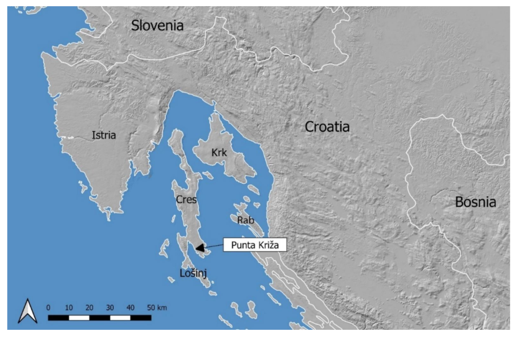
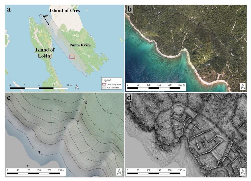
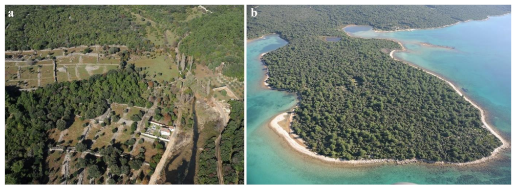
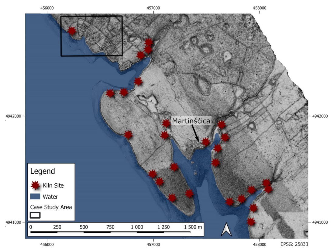
2. Case Study Area at Punta Križa
3. Source Datasets
3.1. ALS Dataset
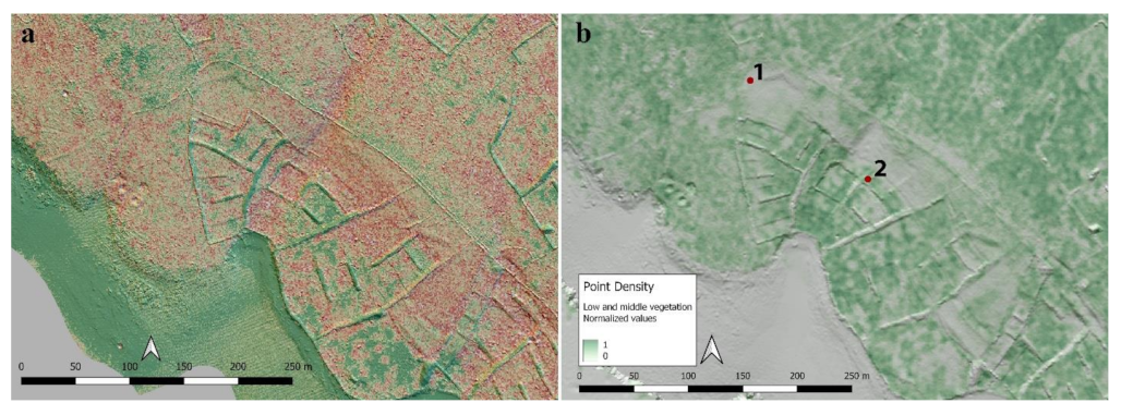
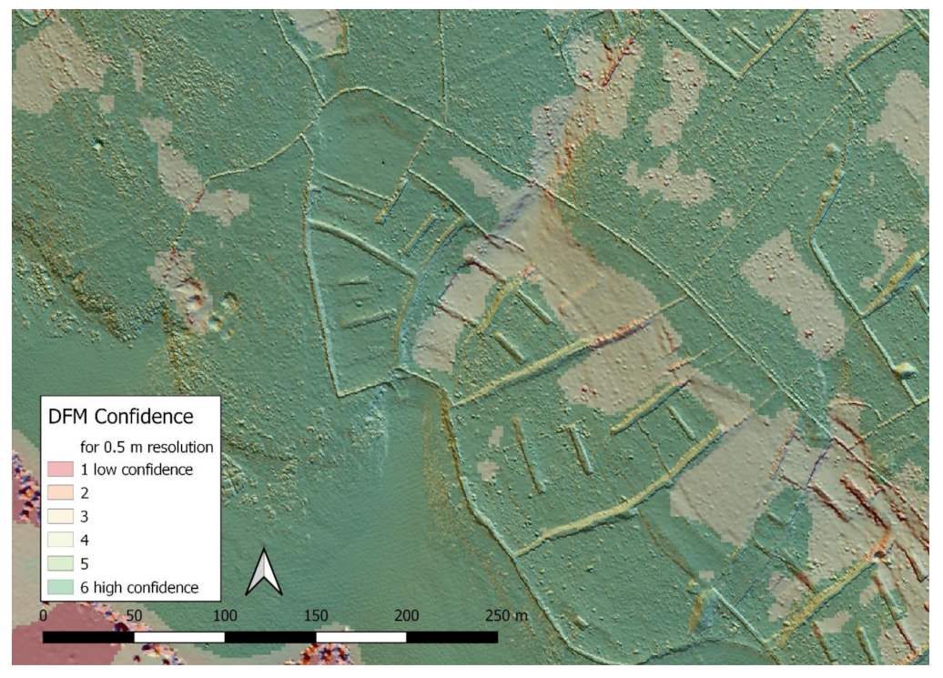
ALS Data Processing
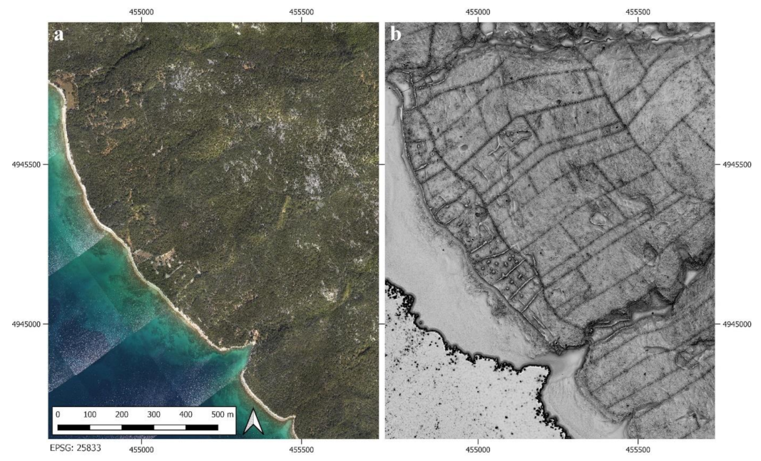
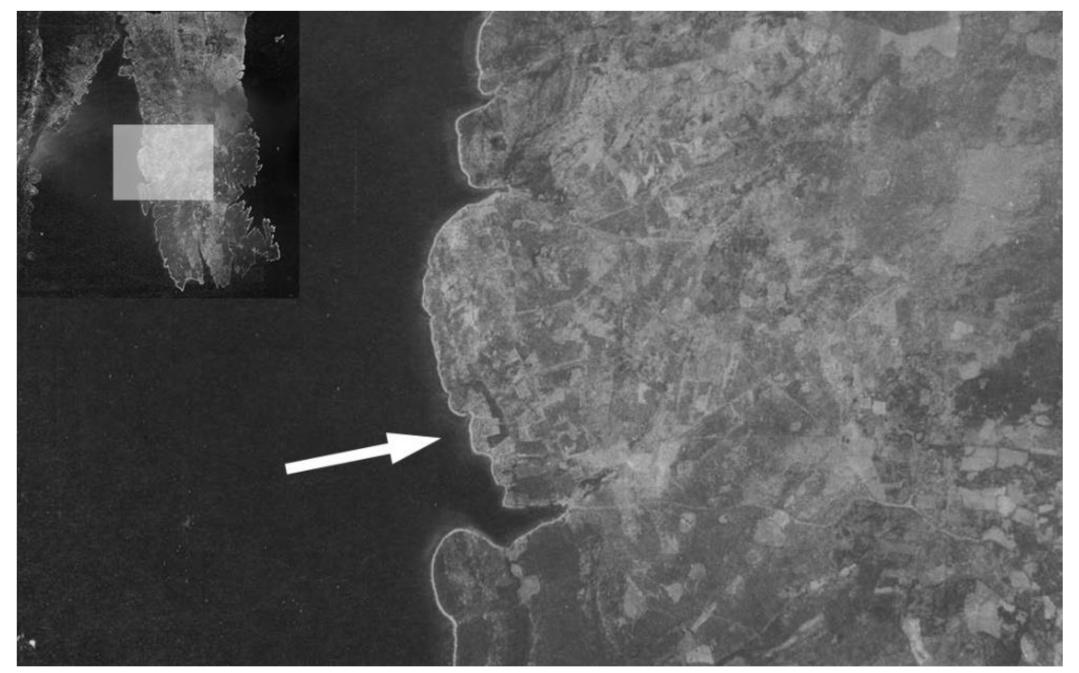
3.2. Aerial Photographs
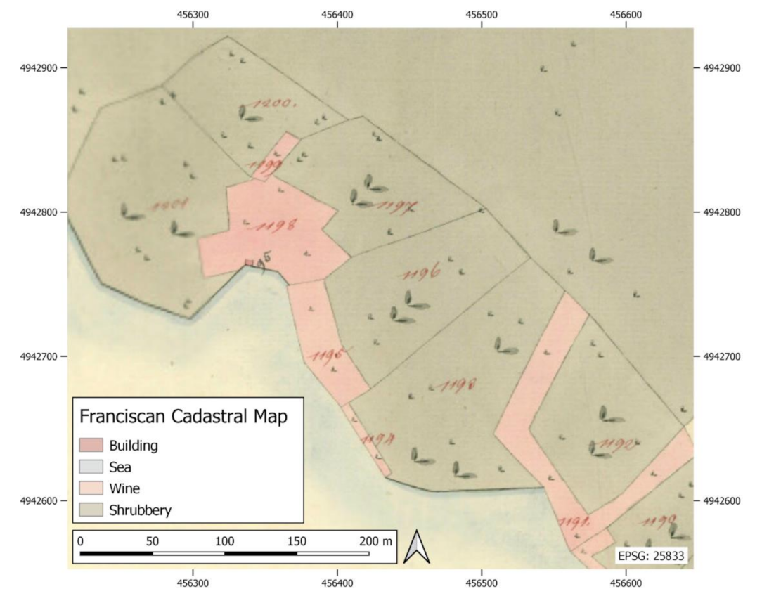
3.3. Historical and Thematic Maps
4. Methods
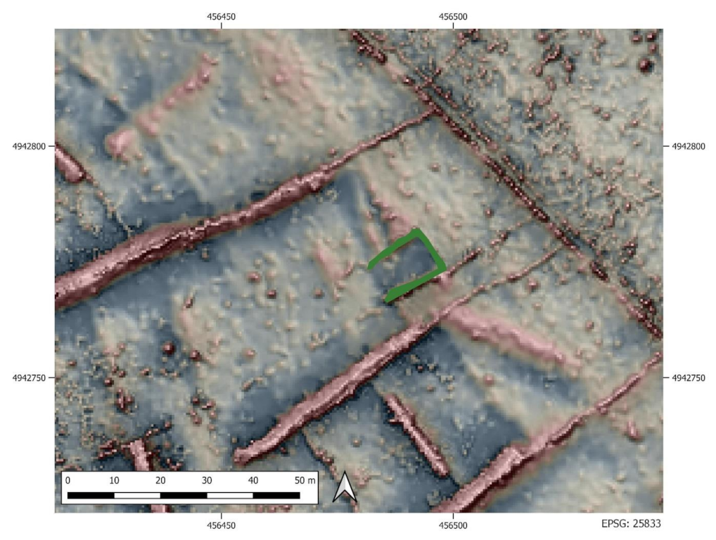
4.1. Preparation of Data for GIS-Based Interpretative Mapping
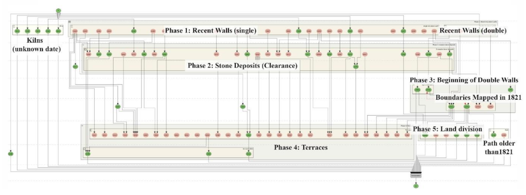
4.2. GIS-Based Interpretative Mapping and Harris Matrix
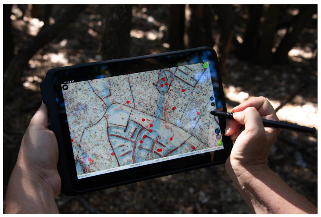
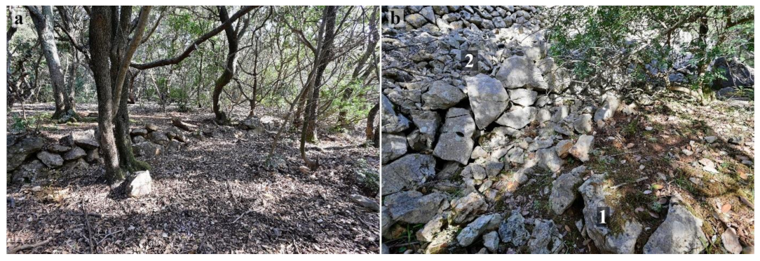
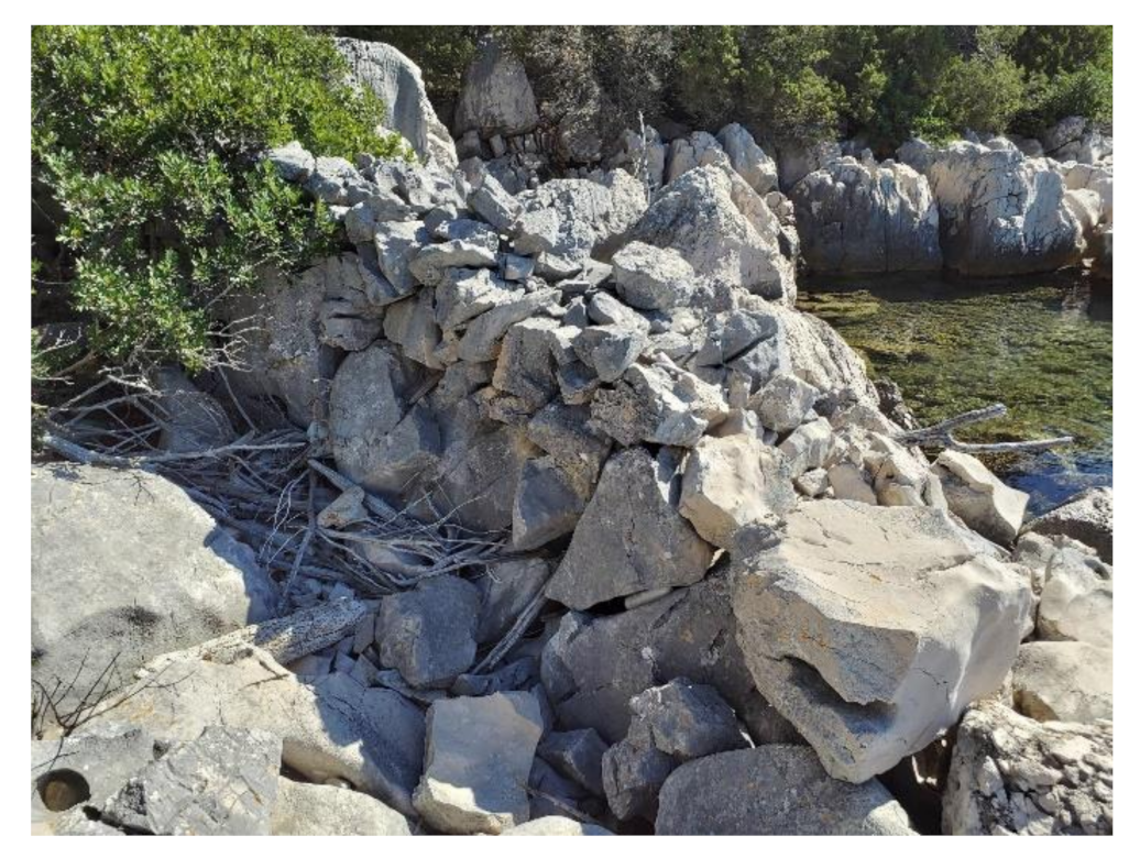
4.3. On-Site Visits
5. Results
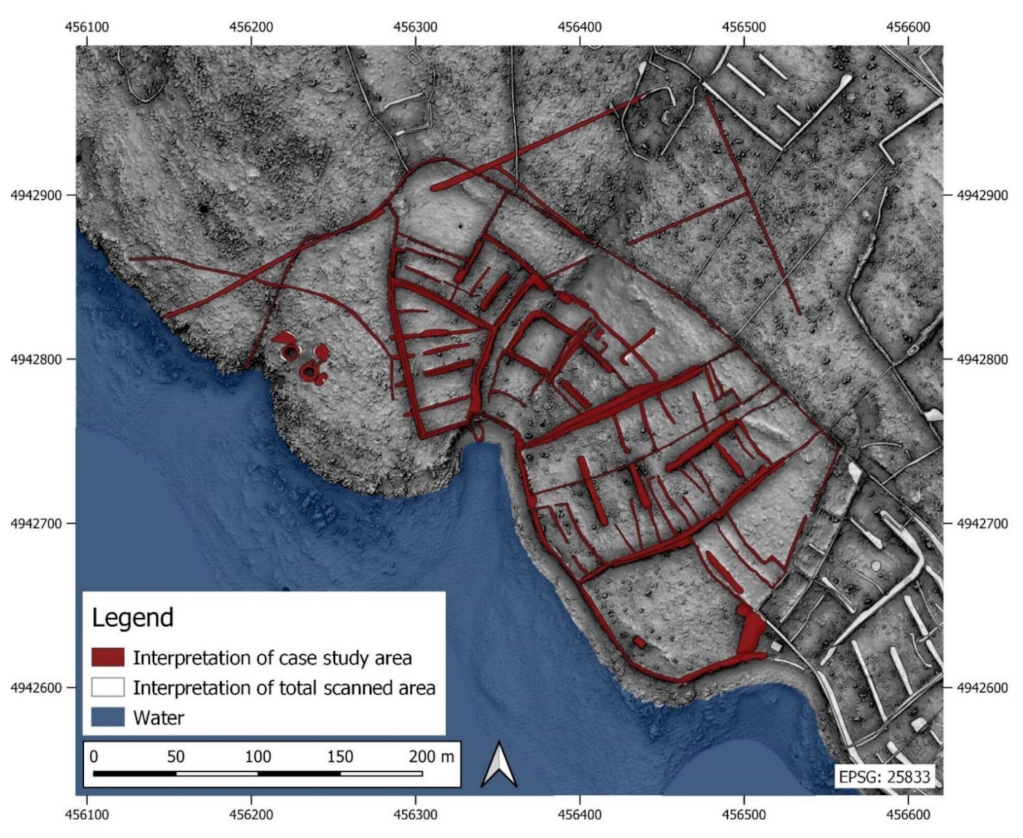
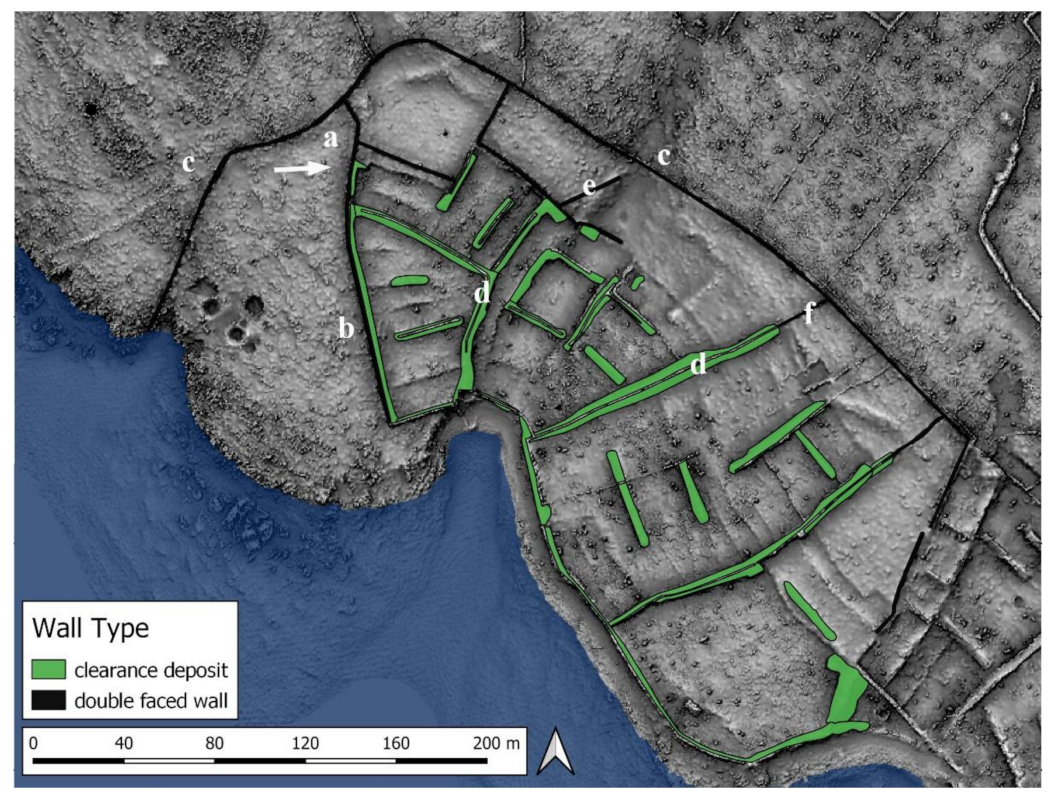
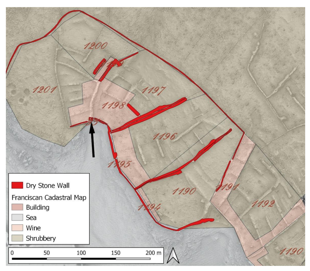
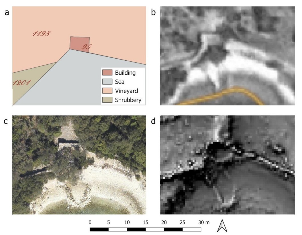
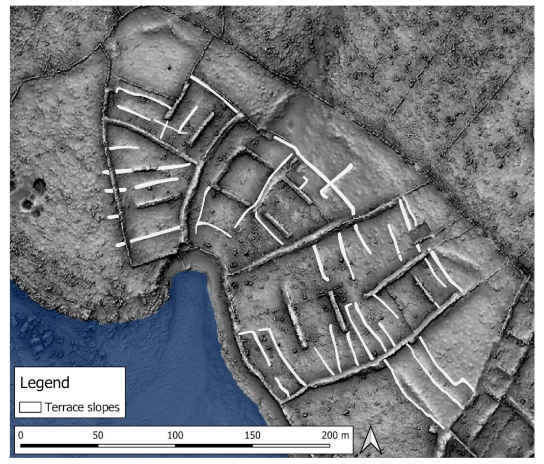
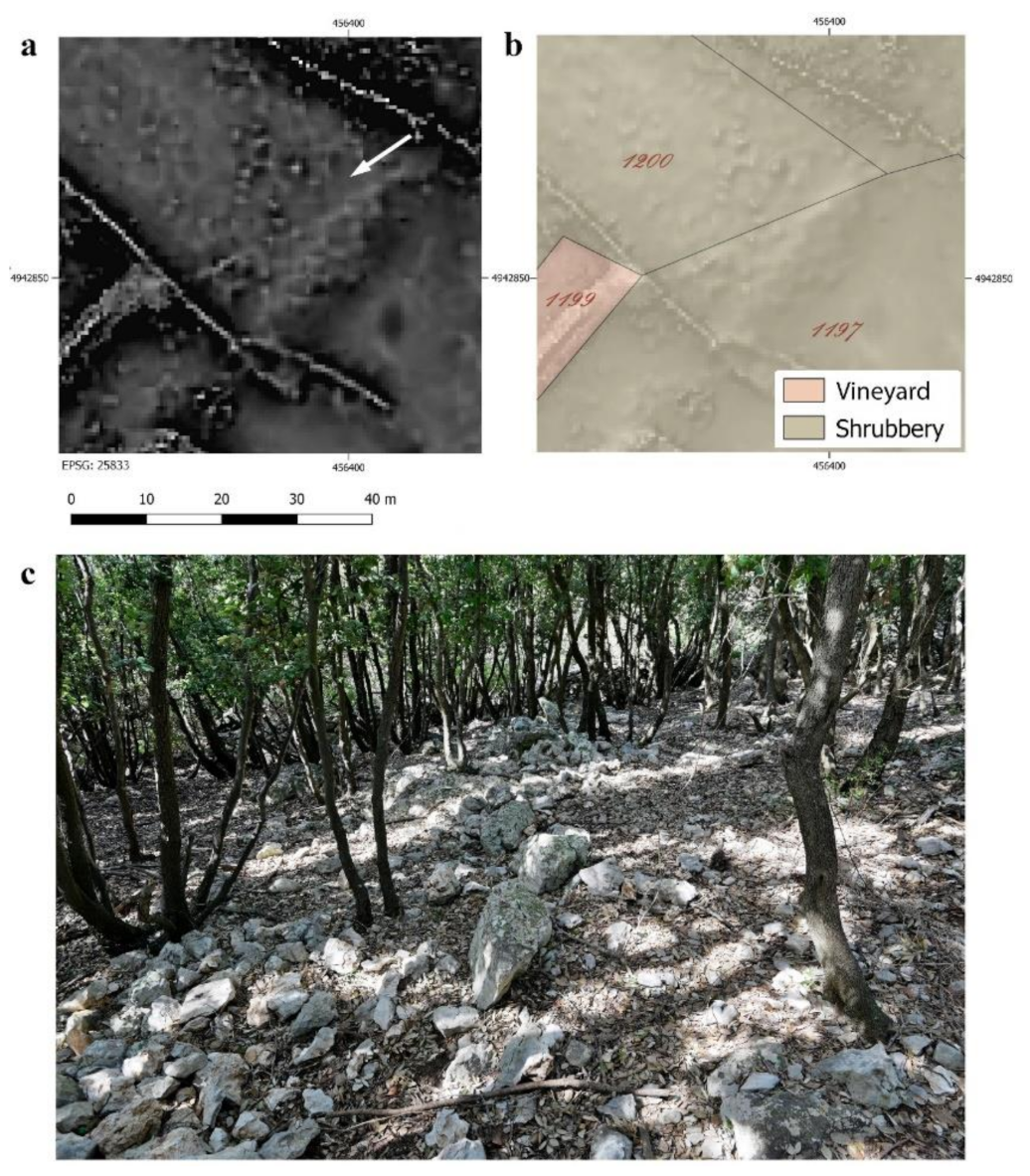
5.1. Interpretative Mapping of the Case Study Area
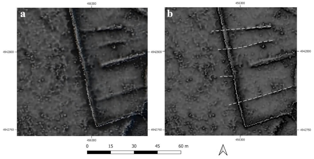
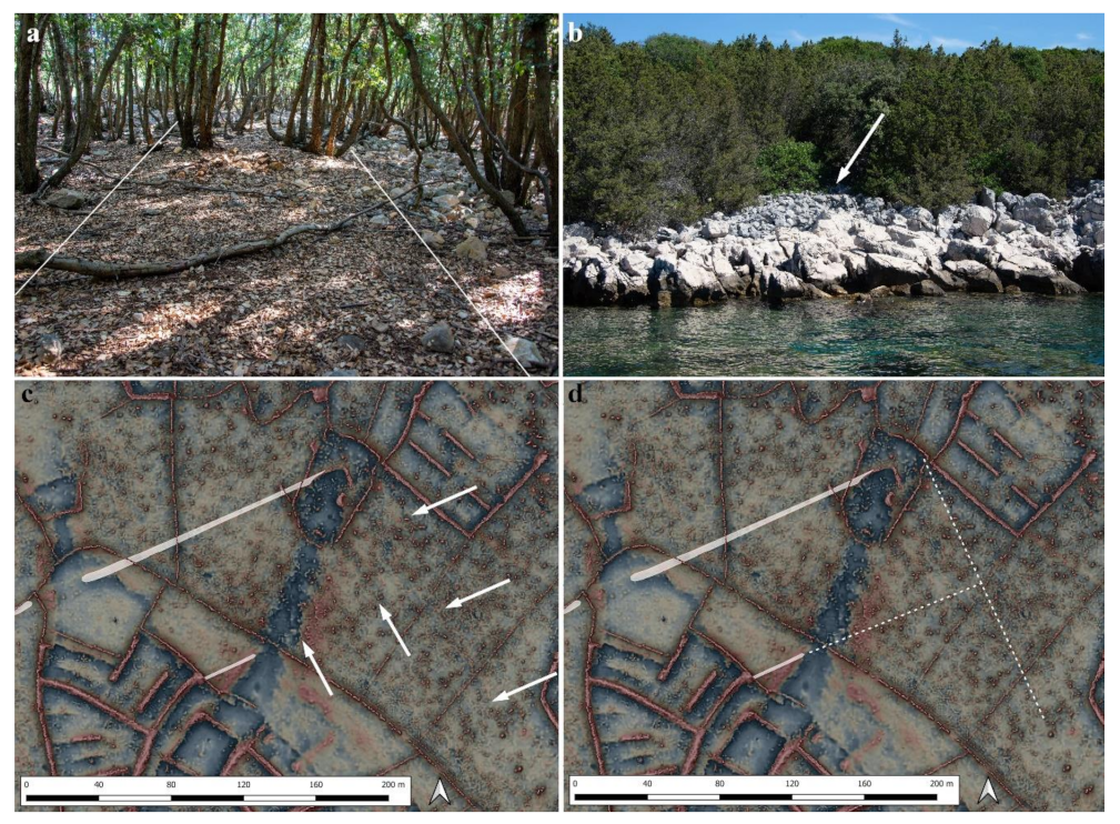
5.1.1. Phase 1: Youngest Dry Stone Walls
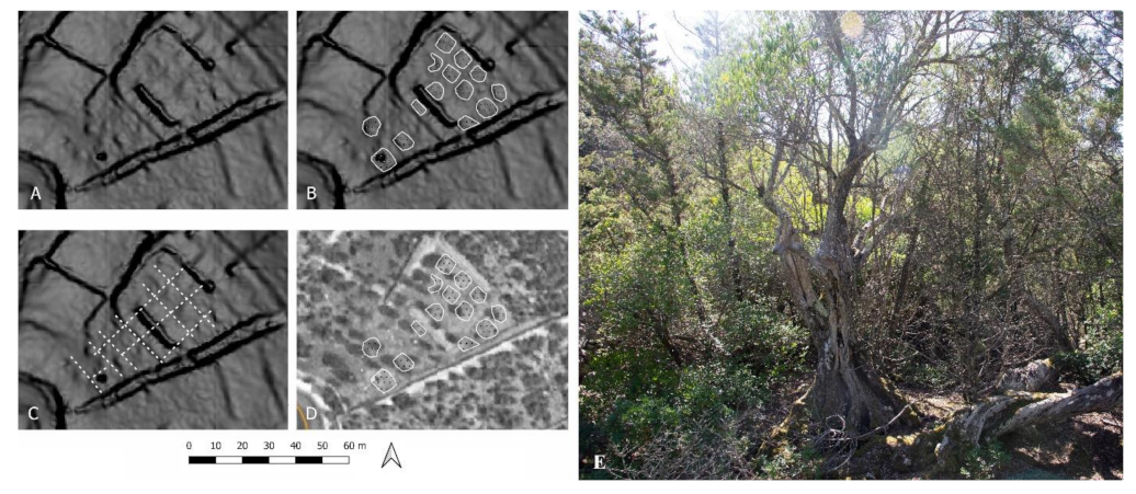
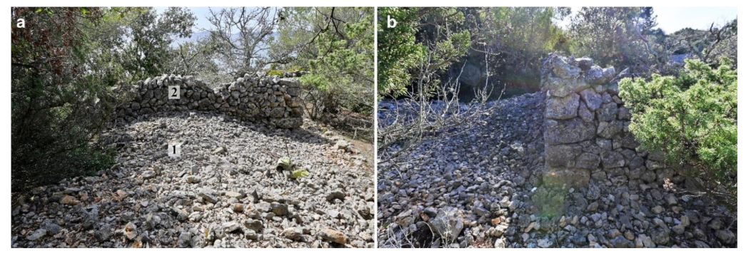
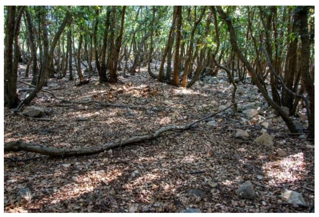
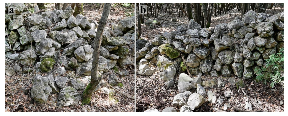
5.1.2. Phase 2: Clearance Deposits
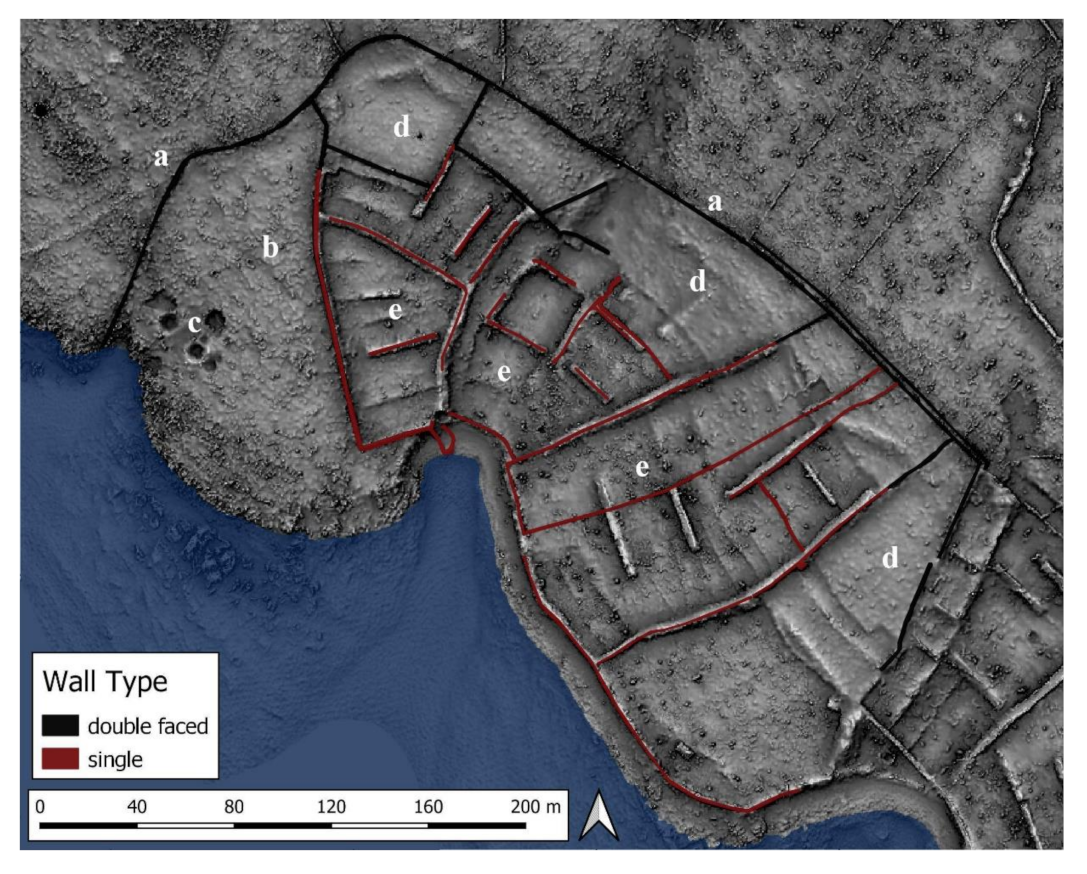
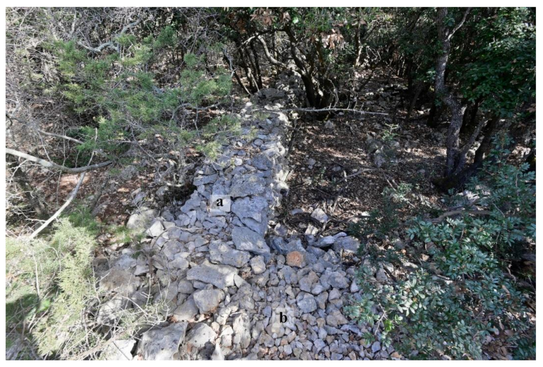
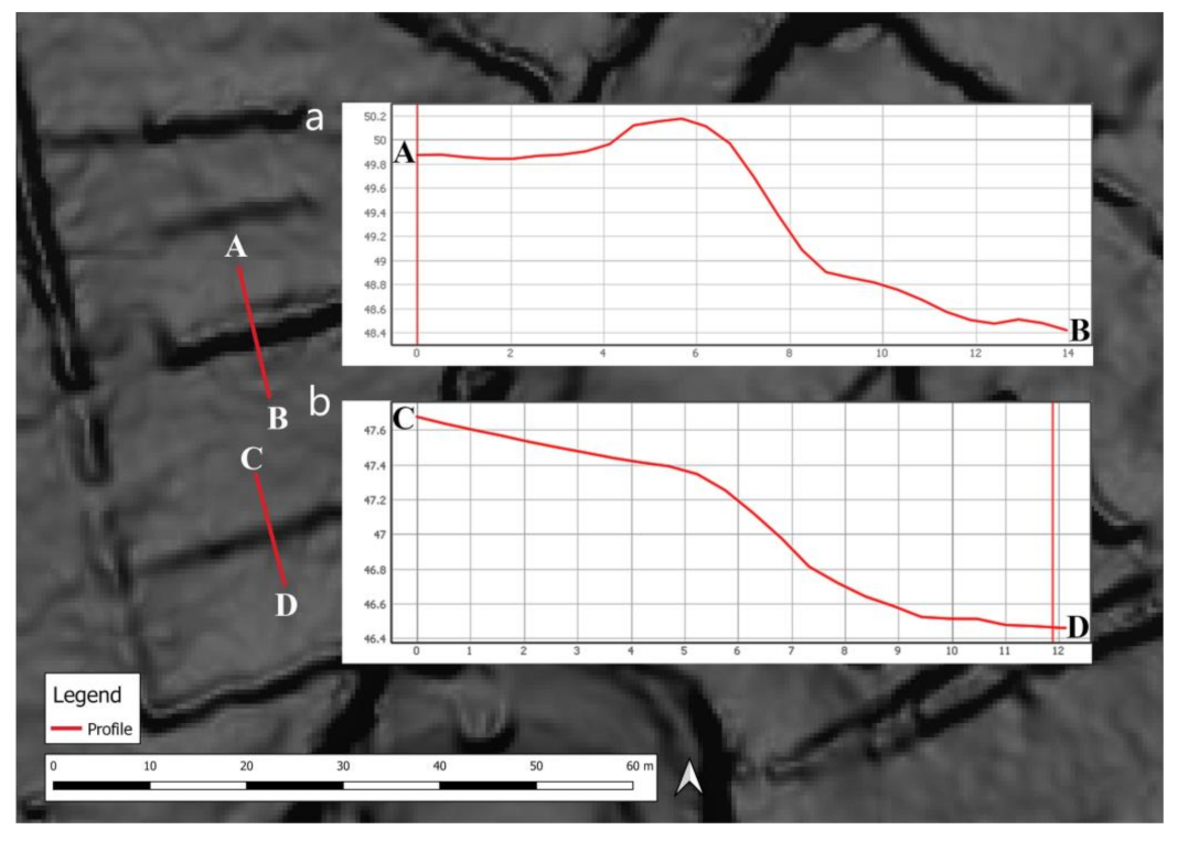
5.1.3. Phase 3: Construction of Double Walls
5.1.4. Phase 4: Terrace Features
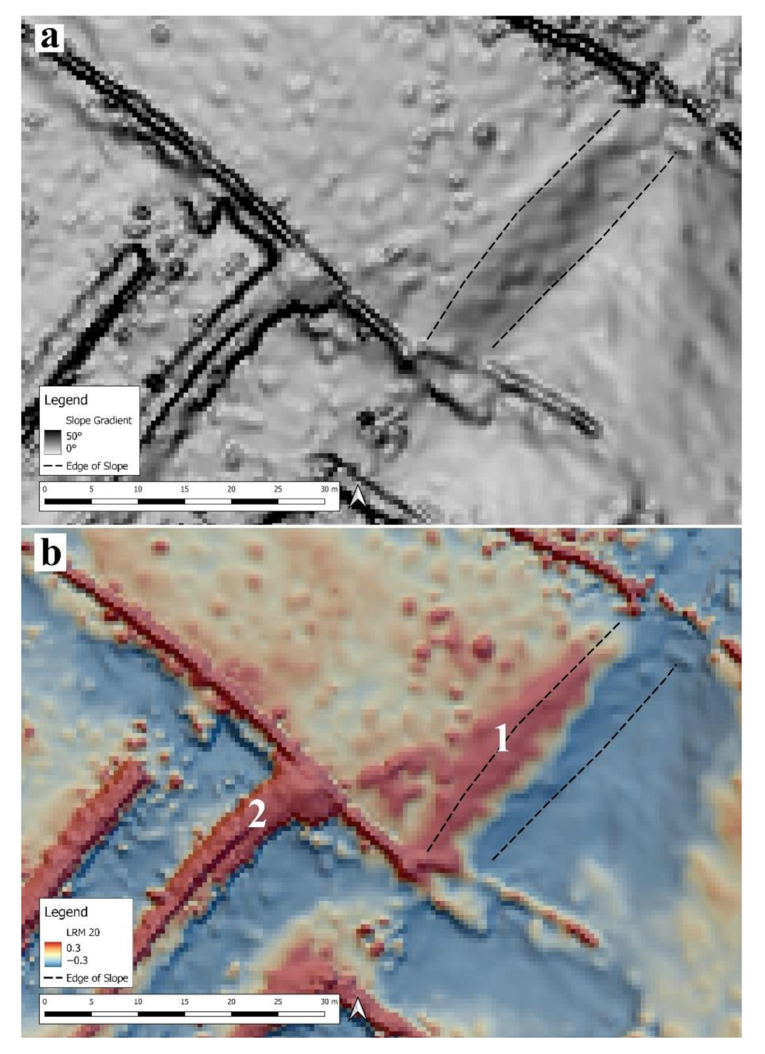
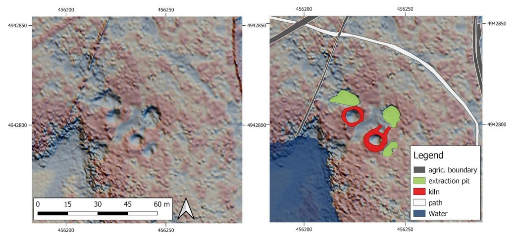
5.1.5. Phase 5: Stratigraphically Oldest Features
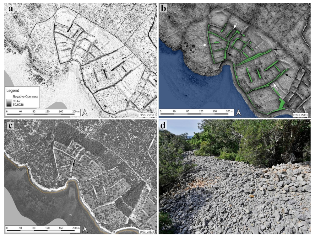
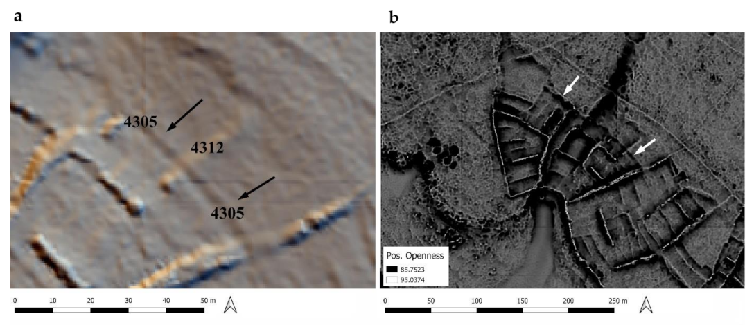
5.1.6. Other Features of Unknown Stratigraphic Phase
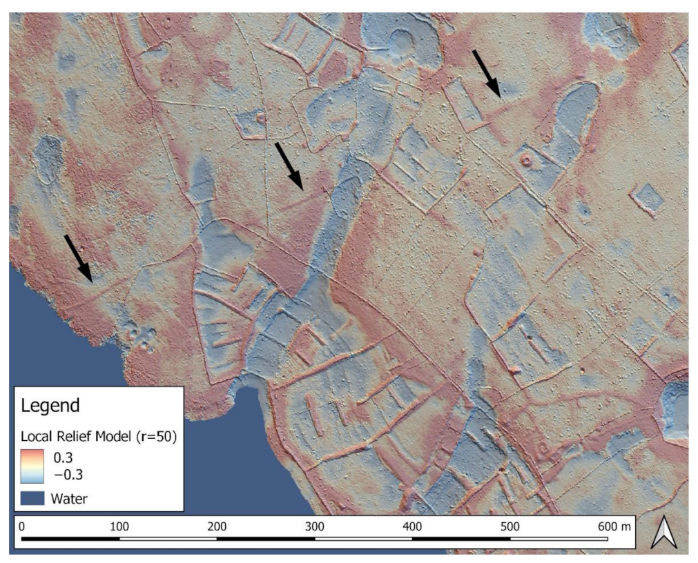
5.2. Results: Putting Things in Context
5.2.1. Phase 5
5.2.2. Phase 4
5.2.3. Phase 3
5.2.4. Phase 2
5.2.5. Phase 1
6. Discussion
7. Conclusions
Author Contributions
Funding
Data Availability Statement
Acknowledgments
Conflicts of Interest
References
- Lewis, P.F. Axioms for Reading the Landscape: Some Guides to the American Scene. In The Interpretation of Ordinary Landscapes; Meinig, D.W., Ed.; Oxford University Press: New York, NY, USA, 1979; pp. 11–32. ISBN 0-19-502536-9. [Google Scholar]
- Rossignol, J.; Wandsnider, L. (Eds.) Space, Time, and Archaeological Landscapes; Springer: Boston, MA, USA, 1992. [Google Scholar]
- Neustupný, E. (Ed.) Space in Prehistoric Bohemia; Institute of Archaeology: Praha, Czech Republic, 1998; ISBN 8086124096. [Google Scholar]
- Banning, E.B. Archaeological Survey; Kluwer Academic/Plenum Publishing: New York, NY, USA, 2002. [Google Scholar]
- Bintliff, J.L. The concepts of ‘site’ and ‘off-site’ archaeology in surface artefact survey. In Non-Destructive Techniques Applied to Landscape Archaeology; Pasquinucci, M., Trément, F., Eds.; Oxbow Books: Oxford, UK, 2000; pp. 200–215. ISBN 978-1900188746. [Google Scholar]
- Varotto, M. (Ed.) World Terraced Landscapes; Springer: Cham, Switzerland, 2019; ISBN 978-3-319-96815-5. [Google Scholar]
- Kremenić, T. Valorisation of the Dry Stone Wall Heritage of the Cres-Lošinj Archipelago. Ph.D. Thesis, University of Padova, Padova, Italy, 2022. [Google Scholar]
- UNESCO. Art of Dry Stone Walling, Knowledge and Techniques. Available online: https://ich.unesco.org/en/RL/art-of-dry-stone-walling-knowledge-and-techniques-01393 (accessed on 15 September 2022).
- Kremenić, T.; Andlar, G.; Varotto, M. How Did Sheep Save the Day? The Role of Dry Stone Wall Heritage and Agropastorality in Historical Landscape Preservation. A Case-Study of the Town of Cres Olive Grove. Land 2021, 10, 978. [Google Scholar] [CrossRef]
- 4 Grada—Dragodid. O Suhozidnoj Baštini i Vještini Gradnje/about Dry Stone Heritage and Construction Skills. Available online: http://www.dragodid.org/ (accessed on 15 September 2022).
- Suhozid.hr. Open Public Inventory of the Croatian Dry Stone Heritage. Available online: www.suhozid.hr (accessed on 15 September 2022).
- Marijanović, B. Pokrovnik—Primjer ograđenoga neolitičkog naselja/Pokrovnik—An Example of an Enclosed Neolithic Settlement. Pril. Inst. Arheol. Zagreb. 2017, 34, 5–44. [Google Scholar]
- Moore, A.M.T. Early Farming in Dalmatia: Pokrovnik and Danilo Bitinj: Two Neolithic Villages in Southeast Europe; Archaeopress Publishing Ltd.: Oxford, UK, 2019; ISBN 978-1-78969-158-0. [Google Scholar]
- Chapman, J.; Shiel, R.; Batović, Š. The Changing Face of Dalmatia: Archaeological and Ecological Studies in a Mediterranean Landscape; Leicester Univ. Press: London, UK, 1996; ISBN 0718500482. [Google Scholar]
- Buršić-Matijašić, K. Gradinska Naselja: Gradine Istre u Vremenu i Prostoru/Klara Buršić-Matijašić; Leykam International: Zagreb, Croatia, 2008; ISBN 978-953-7534-20-2. [Google Scholar]
- Batovič, Š. Benkovački Kraj u Prapovijesti; Matica Hrvatska: Zadar, Croatia, 2004; ISBN 9536419343. [Google Scholar]
- Sirovica, F. Pod near Bruška—Site analysis with a view on prehistoric drywall architecture. Opusc. Archaeol. 2014, 37–38, 50–93. [Google Scholar] [CrossRef]
- Čavić, A. Starogradsko polje kao kultivirani poljoprivredni krajolik kroz povijest (The Field of Stari Grad as a Cultivated Agricultural Landscape Through History). Pril. Povij. Otoka Hvar. 2017, 13, 29–42. [Google Scholar]
- Popović, S.; Bulić, D.; Matijašić, R.; Gerometta, K.; Boschian, G. Roman land division in Istria, Croatia: Historiography, lidar, structural survey and excavations. Mediterr. Archaeol. Archaeom. 2021, 21, 165–178. [Google Scholar] [CrossRef]
- Bradford, J. Ancient Landscapes: Studies in Field Archaeology; Bell & Sons: London, UK, 1957. [Google Scholar]
- Vinci, G.; Bernardini, F.; Furlani, S. Geo-archaeology of the Grozzana area (N–E Italy). J. Maps 2019, 15, 697–707. [Google Scholar] [CrossRef]
- Andlar, G.; Šrajer, F.; Trojanović, A. Classifying the Mediterranean terraced landscape: The case of Adriatic Croatia. Acta Geogr. Slov. 2017, 57, 111–129. [Google Scholar] [CrossRef]
- Andlar, G.; Šrajer, F.; Trojanović, A. Discovering Cultural Landscape in Croatia: History and Classification of Croatian Adriatic Enclosed Landscape. Ann. Ser. Hist. Sociol. 2018, 28, 759–778. [Google Scholar] [CrossRef]
- Benac, Č.; Juračić, M.; Matičec, D.; Ružić, I.; Pikelj, K. Fluviokarst and classical karst: Examples from the Dinarics (Krk Island, Northern Adriatic, Croatia). Geomorphology 2013, 184, 64–73. [Google Scholar] [CrossRef]
- Bognar, A.; Faivre, S.; Buzjak, N.; Pahernik, M.; Bočić, N. Recent Landform Evolution in the Dinaric and Pannonian Regions of Croatia. In Recent Landform Evolution: The Carpatho-Balkan-Dinaric Region; Lóczy, D., Stankoviansky, M., Kotarba, A., Eds.; Springer: Dordrecht, The Netherlands, 2012; pp. 313–344. ISBN 978-94-007-2448-8. [Google Scholar]
- Ford, D.C.; Williams, P.W. Karst Hydrogeology and Geomorphology, Rev. ed.; John Wiley & Sons: Chichester, UK; Hoboken, NJ, USA, 2007; ISBN 9780470849965. [Google Scholar]
- Fuček, L.; Matiček, D.; Vlahović, I.; Oštrić, N.; Prtoljan, B.; Korbar, T.; Husinec, A. Basic Geological Map of the Republic of Croatia, Scale 1:50,000: Sheet Cres 2, (417/2); 1 sheet; Croatian Geological Survey (Department of Geology): Zagreb, Croatia, 2014; ISBN 978-953-6907-26-7. [Google Scholar]
- Lambeck, K.; Anzidei, M.; Antonioli, F.; Benini, A.; Esposito, A. Sea level in Roman time in the Central Mediterranean and implications for recent change. Earth Planet. Sci. Lett. 2004, 224, 563–575. [Google Scholar]
- Faivre, S.; Fouache, E.; Kovačić, V.; Glušćević, S. Geomorphological and archaeological indicators of Croatian shoreline evolution over the last two thousand years. GeoActa Spec. Publ. 2010, 3, 125–133. [Google Scholar]
- Draganits, E.; Gier, S.; Doneus, N.; Doneus, M. Geoarchaeological evaluation of the Roman topography and accessibility by sea of ancient Osor (Cres Island, Croatia). Austrian J. Earth Sci. 2019, 112, 1–19. [Google Scholar] [CrossRef]
- Brunović, D.; Miko, S.; Hasan, O.; Papatheodorou, G.; Ilijanić, N.; Miserocchi, S.; Correggiari, A.; Geraga, M. Late Pleistocene and Holocene paleoenvironmental reconstruction of a drowned karst isolation basin (Lošinj Channel, NE Adriatic Sea). Palaeogeogr. Palaeoclimatol. Palaeoecol. 2020, 544, 109587. [Google Scholar] [CrossRef]
- Dlaka, I.; Križa, P. Prostor, vrijeme ljudi. In Punta Križa. Exhibition Catalog; Lošinjski Muzej, Ed.; Sveučilišne Knjižnice Rijek: Rijeka, Croatia, 2011; pp. 5–17. ISBN 978-953-55837-4-5. [Google Scholar]
- Mirosavljević, V. Jama na Sredi. Arheol. Rad. Raspr. 1959, 1, 131–169. [Google Scholar]
- Starac, R. Arheološka Baština Punte Križe; Exhibition Catalogue Punta Križa; Arheoloski Muzej: Mali Losinj, Croatia, 2011; pp. 19–35. [Google Scholar]
- Ćus-Rukonić, J. Arheološka Topografija Otoka Cresa i Lošinja (Archaeological Topography of the islands of Cres and Lošinj); Izdanja HAD; Hrvatsko Arheolosko Drustvo: Zagreb, Croatia, 1982; Volume 7, pp. 9–17. [Google Scholar]
- Blečić Kavur, M. Get the Balance Right! Osor in Balance of European Cultures and Civilizations in the Last Centuries BC; University of Primorska Press: Koper, Slovenia, 2014; ISBN 978-961-6832-84-7. [Google Scholar]
- Blečić Kavur, M. A Coherence of Perspective: Osor in Cultural Contacts during the Late Iron Age; University of Primorska Press: Koper, Slovenia; Mali Lošinj, Croatia, 2015. [Google Scholar]
- Mohorovičić, A. Pregled i analiza novootkrivenih objekata historijske arhitekture na području grada Osora. Bull. Razreda Likovne Umjet. Jugosl. Akad. Znan. Umjet. 1953, 1–2, 10–16. [Google Scholar]
- Faber, A. Osor-Apsorus iz aspekta antičkog pomorstva. Diadora 1980, 9, 289–317. [Google Scholar]
- Doneus, N.; Doneus, M.; Ettiner-Starčić, Z. The ancient city of Osor, northern Adriatic, in integrated archaeological prospection. Hortus Artium Mediev. 2017, 23, 761–775. [Google Scholar] [CrossRef] [Green Version]
- Čaušević-Bully, M.; Bully, S. Esquisse d’un paysage monastique insulaire dans le nord de l’Adriatique: L’archipel du Kvarner (Croatie). Hortus Artium Mediev. 2013, 19, 167–182. [Google Scholar] [CrossRef]
- Čaušević-Bully, M.; Bully, S.; Delliste, A.; Lefebvre, S.; Mureau, C. Les sites ecclésiaux et monastiques de l’archipel du Kvarner (Croatie), campagne 2019: Martinšćica (île de Cres). Bull. Archéol. Éc. Fr. L’étrang. 2021, 1–47. [Google Scholar] [CrossRef]
- Stražičić, N. Otok Cres. Prilog Poznavanju Geografije Naših Otoka; Otokar Keršovani: Pula, Croatia, 1981. [Google Scholar]
- Gović, V. Povijesne odrednice Puntarskog gospodarstva. In Punta Križa. Exhibition Catalog, Lošinjski Muzej, ed.; Sveučilišne Knjižnice Rijeka: Rijeka, Croatia, 2011; pp. 51–59. ISBN 978-953-55837-4-5. [Google Scholar]
- Gović, V. Organizacija i prostorno oblikovanje pastirskih stanova. In Punta Križa Exhibition Catalog; Lošinjski Muzej, Ed.; Sveučilišne Knjižnice Rijeka: Rijeka, Croatia, 2011; pp. 60–69. ISBN 978-953-55837-4-5. [Google Scholar]
- Margetić, L. Srednjovjekovni Zakoni i Opći Akti na Kvarneru; Nakladni Zavod Globus, Naklada Kvarner, Pravni Fakultet Sveučilišta u Rijeci: Zagreb, Croatia; Rijeka, Croatia, 2012; ISBN 978-953-167-212-2. [Google Scholar]
- Kokalj, Ž.; Somrak, M. Why Not a Single Image? Combining Visualizations to Facilitate Fieldwork and On-Screen Mapping. Remote Sens. 2019, 11, 747. [Google Scholar] [CrossRef]
- Archivio di Stato di Trieste. Catasto di Trieste/Catasto Franceschino/Serie “Mappe des Catasro Franceschino”/Sottoserie—Distritto di Cherso/Sotto-Sottoserie—Commune di Punta Croce. Available online: https://a4view.archiviodistatotrieste.it/patrimonio/2df6e5d3-f760-47c0-b917-1e1a477b2087/sotto-sottoserie-comune-di-punta-croce (accessed on 15 September 2022).
- Državni Zavod za Statistiku. Popis. 2021. Available online: https://popis2021.hr/ (accessed on 15 September 2022).
- Doneus, M.; Doneus, N.; Briese, C.; Pregesbauer, M.; Mandlburger, G.; Verhoeven, G. Airborne Laser Bathymetry—Detecting and recording submerged archaeological sites from the air. J. Archaeol. Sci. 2013, 40, 2136–2151. [Google Scholar] [CrossRef]
- Doneus, M.; Mandlburger, G.; Doneus, N. Archaeological Ground Point Filtering of Airborne Laser Scan Derived Point-Clouds in a Difficult Mediterranean Environment. J. Comput. Appl. Archaeol. 2020, 3, 92–108. [Google Scholar] [CrossRef]
- Lozić, E.; Štular, B. Documentation of Archaeology-Specific Workflow for Airborne LiDAR Data Processing. Geosciences 2021, 11, 26. [Google Scholar] [CrossRef]
- Doneus, M.; Briese, C.; Fera, M.; Janner, M. Archaeological prospection of forested areas using full-waveform airborne laser scanning. J. Archaeol. Sci. 2008, 35, 882–893. [Google Scholar] [CrossRef]
- Kraus, K.; Pfeifer, N. Determination of terrain models in wooded areas with airborne laser scanner data. ISPRS J. Photogramm. Remote Sens. 1998, 53, 193–203. [Google Scholar] [CrossRef]
- Pfeifer, N.; Stadler, P.; Briese, C. Derivation of digital terrain models in the SCOP++ environment. In Proceedings of the OEEPE Workshop on Airborne Laserscanning and Inferometric SAR for Detailed Digital Terrain Models, Stockholm, Sweden, 1–3 March 2001; OEEPE: Stockholm, Sweden, 2001. [Google Scholar]
- Štular, B.; Lozić, E.; Eichert, S. Airborne LiDAR-Derived Digital Elevation Model for Archaeology. Remote Sens. 2021, 13, 1855. [Google Scholar] [CrossRef]
- Štular, B.; Eichert, S.; Lozić, E. Airborne LiDAR Point Cloud Processing for Archaeology. Pipeline and QGIS Toolbox. Remote Sens. 2021, 13, 3225. [Google Scholar] [CrossRef]
- Kraus, K. Interpolation nach kleinsten Quadraten versus Krige-Schätzer. Österr. Zeitschr. Vermess. Geoinf. 1998, 86, 45–48. [Google Scholar]
- Fernandez-Diaz, J.; Carter, W.; Shrestha, R.; Glennie, C. Now You See It… Now You Don’t: Understanding Airborne Mapping LiDAR Collection and Data Product Generation for Archaeological Research in Mesoamerica. Remote Sens. 2014, 6, 9951–10001. [Google Scholar] [CrossRef]
- Zakšek, K.; Oštir, K.; Kokalj, Ž. Sky-View Factor as a Relief Visualization Technique. Remote Sens. Environ. 2011, 3, 398–415. [Google Scholar] [CrossRef]
- Fuhrmann, S. Digitale Historische Geobasisdaten im Bundesamt für Eich- und Vermessungswesen (BEV). Die Urmappe des Franziszeischen Kataster. Vermess. Geoinf. 2007, 95, 24–35. [Google Scholar]
- Timár, G.; Biszak, S.; Székely, B.; Molnár, G. Digitized Maps of the Habsburg Military Surveys—Overview of the Project of ARCANUM Ltd. (Hungary). In Preservation in Digital Cartography: Archiving Aspects, 1st ed.; Jobst, M., Ed.; Springer: Berlin, Germany, 2010; pp. 273–283. ISBN 978-3-642-12733-5. [Google Scholar]
- Third Military Survey of the Habsburg Empire. Available online: https://maps.arcanum.com/de/map/europe-19century-thirdsurvey (accessed on 15 September 2022).
- Državna Geodetska Uprava. Croatian Base Map 1:5000. Available online: https://geoportal.dgu.hr/metadataeditor/apps/metadataui/print.html?uuid=21cededd-5101-4f28-ad57-f08fcf7c491a&currTab=simple&hl=hrv (accessed on 15 September 2022).
- ARKOD. Agencija za Plaćanja u Poljoprivredi, Ribarstvu i Ruralnom Razvoju. Available online: http://preglednik.arkod.hr/ (accessed on 10 February 2021).
- Verhoeven, G.J. Mesh Is More—Using All Geometric Dimensions for the Archaeological Analysis and Interpretative Mapping of 3D Surfaces. J. Archaeol. Method Theory 2017, 24, 999–1033. [Google Scholar] [CrossRef]
- Štular, B.; Lozić, E. Comparison of Filters for Archaeology-Specific Ground Extraction from Airborne LiDAR Point Clouds. Remote Sens. 2020, 12, 3025. [Google Scholar] [CrossRef]
- Grammer, B.; Draganits, E.; Gretscher, M.; Muss, U. LiDAR-guided Archaeological Survey of a Mediterranean Landscape: Lessons from the Ancient Greek Polis of Kolophon (Ionia, Western Anatolia). Archaeol. Prospect. 2017, 24, 311–333. [Google Scholar] [CrossRef]
- Doneus, M.; Briese, C. Airborne Laser Scanning in Forested Areas—Potential and Limitations of an Archaeological Prospection Technique. In Remote Sensing for Archaeological Heritage Management, Proceedings of the 11th EAC Heritage Management Symposium, Reykjavik, Iceland, 25–27 March 2010; Cowley, D., Ed.; Archaeolingua, EAC: Budapest, Hungary, 2011; pp. 53–76. ISBN 978-963-9911-20-8. [Google Scholar]
- Neubauer, W.; Traxler, C.; Bornik, A.; Lenzhofer, A. Stratigraphy from topography I: Theoretical and practical considerations for the application of the Harris Matrix for the GIS-based spatio-temporal archaeological interpretation of topographical data. Archaeol. Austriaca 2022, 106. in print. [Google Scholar]
- Doneus, M.; Neubauer, W.; Filzwieser, R.; Sevara, C. Stratigraphy from Topography II—The practical application of the Harris Matrix for the GIS-based spatio-temporal archaeological interpretation of topographical data. Archaeol. Austriaca 2022, 106. in print. [Google Scholar]
- Harris, E.C. Principles of Archaeological Stratigraphy, 2nd ed.; Academic Press: London, UK, 1989. [Google Scholar]
- Traxler, C.; Neubauer, W. The Harris Matrix Composer—A New Tool to Manage Archaeological Stratigraphy. In Digital Heritage, Proceedings of the 14th International Conference on Virtual Systems and Multimedia, Limassol, Cyprus, 20–25 October 2008; Ioannides, M., Ed.; Archaeolingua: Budapest, Hungary, 2008; pp. 13–20. ISBN 978-963-9911-00-0. [Google Scholar]
- Hesse, R. LiDAR-derived Local Relief Models—A new tool for archaeological prospection. Archaeol. Prospect. 2010, 17, 67–72. [Google Scholar] [CrossRef]
- Software: QField; The QField Project/OPENGIS.ch. 2019. Available online: https://qfield.org/ (accessed on 15 September 2022).
- Antonson, H. Revisiting the “Reading Landscape Backwards” Approach: Advantages, Disadvantages, and Use of the Retrogressive Method. Rural. Landsc. Soc. Environ. Hist. 2018, 5, 4. [Google Scholar] [CrossRef]
- Archivio di Stato di Trieste. Serie—“Mappe del Catasto Franceschino”. Available online: https://a4view.archiviodistatotrieste.it/patrimonio/85ea26bb-a430-4ac7-b9c4-1019f2bfea90/383-b-14-mappa-catastale-del-comune-di-punta-croce-foglio-xii-sezione-xiv-1821-sec-xix-primo-quarto (accessed on 15 September 2022).
- Turner, S.; Kinnaird, T.; Varinlioğlu, G.; Şerifoğlu, T.; Koparal, E.; Demirciler, V.; Athanassoulis, D.; Ødegård, K.; Crow, J.; Jackson, M.J.B.; et al. Agricultural terraces in the Mediterranean: Intensive construction during the later Middle Ages revealed by landscape analysis with OSL profiling and dating. Antiquity 2021, 95, 773–790. [Google Scholar] [CrossRef]
- Faričić, J.; Juran, K. Human Footprints in the Karst Landscape: The Influence of Lime Production on the Landscape of the Northern Dalmatian Islands (Croatia). Geosciences 2021, 11, 303. [Google Scholar] [CrossRef]
- Bulić, D. Rimska centurijacija Istre. Tabula 2012, 10, 50–74. [Google Scholar] [CrossRef] [Green Version]
- Marchiori, A. Infrastrutture Territoriale e Strutture Insediamente Dell’Istria Romana: La Divisione Centuriale di Pola e Parenzo in Rapporto ai Grandi Complessi Costieri Istriani. Il Caso Nord Parentino. Ph.D. Thesis, Università degli Studi di Padova, Padova, Italy, 2010. [Google Scholar]
- Suić, M. Limitacija agera rimskih kolonija na istočnoj jadranskoj obali. Zb. Rad. Inst. Hist. Nauk. Zadru 1955, 1, 1–36. [Google Scholar]
- Starac, A. Rimsko Vladanje u Histriji i Liburniji II.: Društveno i Pravno Uredenje Prema Literarnoj Natpisnoj i Arheološkoj Gradi; Arheološki Muzej Istre: Pula, Croatia, 2000; ISBN 9536153114. [Google Scholar]
- Kadi, M. Centurijacija kopnenog dijela agera rimske kolonije Jadera (Zadar). Rimski katastar. (Centuriation of Continental Part of Iader (Zadar) Roman Colony. Ager Roman cadastre.). Kartogr. Geoinf. 2020, 19, 106–111. [Google Scholar]
- Campbell, B. Shaping the Rural Environment: Surveyors in Ancient Rome. J. Rom. Stud. 1996, 86, 74–99. [Google Scholar] [CrossRef]
- Banaszek, Ł.; Cowley, D.; Middleton, M. Towards National Archaeological Mapping. Assessing Source Data and Methodology—A Case Study from Scotland. Geosciences 2018, 8, 272. [Google Scholar] [CrossRef]
- Cowley, D.; Banaszek, Ł.; Geddes, G.; Gannon, A.R.; Middleton, M.; Millican, K. Making LiGHT Work of Large Area Survey? Developing Approaches to Rapid Archaeological Mapping and the Creation of Systematic National-scaled Heritage Data. J. Comput. Appl. Archaeol. 2020, 3, 109–121. [Google Scholar] [CrossRef] [Green Version]
- Cowley, D. What do the patterns mean? Archaeological distributions and bias in survey data. In Digital Methods and Remote Sensing in Archaeology: Archaeology in the Age of Sensing; Forte, M., Campana, S., Eds.; Springer International Publishing: Cham, Switzerland, 2017; pp. 147–170. ISBN 9783319406589. [Google Scholar]
- Cosgrove, D. Geography and Vision: Seeing, Imagining and Representing the World; I.B. Tauris: London, UK, 2008; ISBN 9781850438465. [Google Scholar]
- Mlekuž, D. Messy landscapes: Lidar and the practices of landscaping. In Interpreting Archaeological Topography: Airborne Laser Scanning, 3D Data and Ground Observation; Opitz, R.S., Cowley, D., Eds.; Oxbow Books: Oxford, UK, 2013; pp. 88–99. ISBN 978-1-84217-516-3. [Google Scholar]


| Title | Harbours and Landing Places on the Balkan Coasts of Byzantine Empire (4th to 12th Centuries). Technology and Monuments, Economic and Communication. |
|---|---|
| Purpose | Archaeology (combined land and underwater survey) |
| Date | 29 March 2012 |
| Operator | Airborne Technologies |
| Scanner type | Full-waveform with online waveform processing |
| Instrument | RIEGL VQ-820-G |
| Pulse repetition rate | 200 kHz |
| Wavelength | 532 nm |
| Scanning angle | 60° |
| Additional sensors | IGI Digicam H-39 |
| Altitude above ground | 450 m |
| Flight strip overlap | 70% |
| Footprint diameter | 0.45 m |
| Average laser pulse density per m2 | 16 |
| Average ground points per m2 | 5.1 (“dense_veg.”)–5.5 (“stone_wall”) |
| LAS format | 1.2 |
| Coordinate System | EPSG:25833–ETRS89/UTM zone 33N |
| Strip Adjustment | Yes, using OPALS |
| Ground-point filtering | SCOP++ |
| Steps | Step Name | Parameters | “stone_wall” | “dense_veg” | |
|---|---|---|---|---|---|
| 1 | Step 1 | ThinOut | Cell size: | 2 | 3 |
| Thinning method | lowest | k-th lowest | |||
| Level k: | -- | 3 | |||
| Step 2 | Filter | Lower branch | 0.35; 0.35; 1.0 | 0.35; 0.35; 1.0 | |
| Upper branch: | 0.1; 0.3; 0.6 | 0.05; 0.05; 0.1 | |||
| Trend | On | below | |||
| Prediction | below | below | |||
| Penetration rate | 20% | 40% | |||
| Interpolation | Grid width: 0.5 m CU:20 Covariance function: bell curve | Grid width: 1.5 m CU:20 Covariance function: bell curve | |||
| Step 3 | SortOut | Upper distance | 1.6 | 3.0 | |
| Lower distance | none | 3.0 | |||
| Slope dependency | none | 2.0 | |||
| 2 | Step 4 | ThinOut | Cell size: | 0.3 | 1.5 |
| Thinning method | lowest | k-th lowest | |||
| Level k: | -- | 2 | |||
| Step 5 | Filter | Lower branch | 0.35; 0.35; 1.0 | 0.35; 0.35; 1.0 | |
| Upper branch: | 0.1; 0.3; 0.6 | 0.05; 0.05; 0.1 | |||
| Trend | On | Below | |||
| Prediction | Below | Below | |||
| Penetration rate | 20% | 40% | |||
| Interpolation | Grid width: 0.25 CU:20 CF: bell curve | Grid width: 0.7 CU:20 CF: bell curve | |||
| Step 6 | SortOut | Upper distance | -- | 1.0 | |
| Lower distance | -- | 3.0 | |||
| Slope dependency | -- | 2.0 | |||
| 3 | Step 7 | ThinOut | Cell size: | -- | 0.5 |
| Thinning method | -- | lowest | |||
| Step 8 | Filter | Lower branch | -- | 0.35; 0.35; 1.0 | |
| Upper branch: | -- | 0.05; 0.05; 0.1 | |||
| Trend | -- | Below | |||
| Prediction | -- | Below | |||
| Penetration rate | -- | 40% | |||
| Interpolation | -- | Grid width: 0.25 CU:20 CF: bell curve | |||
| Step 9 | Fill Void Areas | Sampling Interval | -- | 2.0 | |
| Filling Method | -- | Linear Prediction | |||
| Bridging Distance | -- | 42.0 | |||
| Step 10 | Interpolate | Grid width: | 0.5 | 0.5 | |
| CU: | 25 | 25 | |||
| Covariance function: | adapting | adapting | |||
| 5 | Step 11 | Classify | Output format | las | las |
| High vegetation | 5.0 | 5.0 | |||
| Medium vegetation | 1.0 | 1.0 | |||
| Low vegetation | 0.25 | 0.25 | |||
| ground | |||||
| Below DTM | −0.25 | −0.25 | |||
| Slope dependency | -- | -- |
| Field Name | Description |
|---|---|
| SU | Stratigraphic Unit—unique identifier that also linked to the stratigraphic unit of the Harris Matrix Composer. |
| Description | drop-down list with a descriptive parameter, including sunken feature, wall, slope, mound, bank, deposit |
| Interpretation | functional classification, as, e.g., agricultural boundary, enclosure, building, kiln, path. |
| Wall type | characterization of the type of a dry stone wall |
| Group | name of grouped features assigned during interpretation |
| Phase | chronological phase (a field filled at a late stage in mapping when phasing has been completed. |
| Basemap/Fr. Cad. Map/1953 | Boolean fields specifying visibility of features on respective sources. |
| Confidence | Subjective value indicating the confidence of the interpretation (Values 1–3, where 1 = questionable; 2 = likely; 3 = confident). |
| Visualization | the source visualization(s) from which a feature was mapped |
| Comment | free text field for additional information |
| Is Above | SU-identifier of all features that are cut by the current feature. |
| Is Below | SU-identifier of all features that overlie the current feature. |
Publisher’s Note: MDPI stays neutral with regard to jurisdictional claims in published maps and institutional affiliations. |
© 2022 by the authors. Licensee MDPI, Basel, Switzerland. This article is an open access article distributed under the terms and conditions of the Creative Commons Attribution (CC BY) license (https://creativecommons.org/licenses/by/4.0/).
Share and Cite
Doneus, M.; Doneus, N.; Cowley, D. Confronting Complexity: Interpretation of a Dry Stone Walled Landscape on the Island of Cres, Croatia. Land 2022, 11, 1672. https://doi.org/10.3390/land11101672
Doneus M, Doneus N, Cowley D. Confronting Complexity: Interpretation of a Dry Stone Walled Landscape on the Island of Cres, Croatia. Land. 2022; 11(10):1672. https://doi.org/10.3390/land11101672
Chicago/Turabian StyleDoneus, Michael, Nives Doneus, and Dave Cowley. 2022. "Confronting Complexity: Interpretation of a Dry Stone Walled Landscape on the Island of Cres, Croatia" Land 11, no. 10: 1672. https://doi.org/10.3390/land11101672