Landscape Changes in the Southern Coalfields of West Virginia: Multi-Level Intensity Analysis and Surface Mining Transitions in the Headwaters of the Coal River from 1976 to 2016

Abstract

This study analyzes land-cover transitions in the headwaters of the Big Coal River in the Central Appalachian Region of the US, from 1976 to 2016, where surface mining was found as the major driver of landscape change. The land-change analysis combined Multi-Level Intensity Analysis for two-time intervals (1976–1996, 1996–2016) with Difference Components, to differentiate suspected misclassification errors from actual changes. Two land cover classifications were obtained with segmentation analysis and machine learning algorithms from historical high-resolution aerial images and ancillary data. Intensity Analysis allowed for the inspection of transitions across five land cover (LC) classes and measure the degree of non-stationarity of land change patterns. Results found surface mining-related classes and their transitions, including the effects of reclamation processes on areas mined before the enactment of the Surface Mining Control and Reclamation Act (SMCRA, 1977). Results included changes in settlement distribution, low vegetation, water bodies, and forest class transitions. The findings can be applied to infer similar land-change processes in the more extensive Appalachian region where Mountain Top Removal (MTR) operations are widespread. The overall method can be used to address similar problems and inform landscape managers with detailed data to support land use alternatives and conservation in regions that experienced intense changes and are characterized by anthropogenic disturbances and novel ecosystems.

1. Introduction

This study presents the findings of a land-change analysis conducted in the headwaters of the Coal river, during a 40 year interval, from 1976 to 1996. This is a subwatershed located in the central Appalachian coalfields region of the US [1,2], within the southern coalfields of West Virginia (WV) [3] (Figure 3). The land change processes in this area are of particular interest for the land-change transitions associated with surface mining and Mountain Top Removal (MTR). The overall knowledge derived by the analysis of the land change processes can be relevant for characterizing the region’s landscape with information concerning the biophysical structure and function of ecosystems [4] through the identification of specific land cover (LC) transitions and classes.

The study’s main objective is to address landscape changes in the study area and test the stationarity of land transitions applying a post classification comparison (PCC) method based on five relevant LC classes. To achieve this goal, the Multi-Level Intensity Land-change Analysis method [5] was applied to examine land-change processes in the Headwaters of the Coal River using high-resolution images (1–2 m) across two time intervals (1976–1996 and 1996–2016) spanning a total of 40 years. The comparison of the magnitude of the errors at each time point with the magnitude of temporal differences [6] applied in this study enabled the identification of the potential sources of errors to avoid misinterpretations of the land-change analysis results. Three land cover classifications (LCCs), consisting of five classes (developed areas, barren land, water, low vegetation, and forest), were derived from 1 and 2 m spatial resolution imagery over three time points (1976, 1996, and 2016). The 1976 and 1996 LCCs were derived for this study.

Since surface coal mining represented the principal driver of land change in the Central Appalachians [7], the study objective was to address how its effects spread out on the landscape, and how those effects could intersect or interact with other landscape dynamics [8,9] that the exploratory nature of this study may reveal in the study area, due to the complex environmental history of the region [10,11,12,13,14,15,16]. A secondary goal was to update the extent of surface mining in the study area from 1976 and compare our results with the findings obtained by other research [17].

2. Background

2.1. Surface Coal Mining in Central Appalachians

In the Central Appalachian region surface mining has been a massive driver of land change and ecosystem alteration due to the scale of the operations and a lengthy history [17]. Coal surface mining has been identified as the main driver of landscape changes in the region and its diffusion was the greatest cause of net forest loss and conversion over the last four decades [18]. Its effects have been compared to those of extra-urban development in the rest of the eastern US [7,19]. In the last decades, Mountaintop Removal and Valley Fills (MTR, MTRVF) has drawn the attention of the scientific community due to its deep impacts on ecosystems, landscapes, human and natural communities [20,21,22,23]. Nevertheless, MTRVF (Figure 1c) represents only the latest phase of surface mining in Central Appalachians, and its effects can compound those of legacy surface mining (e.g., strip mining or contour mining, auger mining, and highwall mining) [24].

Large-scale surface coal mining in WV started after 1914, while the first surface mining reported in the region opened in eastern Kentucky in 1905 [25]. From 1936 the mechanization process registered a rapid advancement with a consistent growth after the mid of 1950s thanks to the development of giant shovels and draglines [26]. A large quantity of strip mining was produced after the 1940s, during the war effort, due to the increased coal demand and labor shortage. Strip mines presented highly mechanized operations, for this reason, they were less dependent on hand labor [27,28]. The estimated area of strip-mined land in WV in 1950 was close to 50,000 acres (20,234.3 hectares). In 1939 WV adopted the first regulatory legislation due to the problems generated by surface mining [25], while in 1945, a legislative act introduced several procedures for the reclamation of formerly mined land; like land regrading and drainage, and the planting of trees, shrub and grasses [29]. By the beginning of the 1950s, surface mining activities attracted growing attention due to the environmental problems produced [25,29]. The 1970s represented the moment in which strip-mined areas reached another peak in the region [30,31]. An aerial survey of 1964 in Kentucky’s eastern mining region indicated that about 12% of the surface mining areas were characterized by landslides [32]. In WV, the worst flood event derived from surface mining operations occurred in 1972; it was the Buffalo Creek Flood Disaster in Logan County, where 125 people died due to the collapse of a coal dam impoundment [33,34].

The Clean Water Act of 1972 (CWA, 33 U.S.C. §1252) and the Surface Mining Control and Reclamation Act of 1977 (SMCRA, 30 U.S.C. §1201) represented a turning point for the US surface coal mining history. The SMCRA consistently readdressed, from individual state regulation to the federal level, the policies that drove the socio-technical processes of coal extraction, mine reclamation, and environmental regulation.

The SMCRA established the restoration of mining areas introducing the principle of “approximate original contour” (AOC), to eliminate the highwalls and the mining spoil for stabilizing potentially unstable terrain slopes [32]. Another requirement consisted in reclaiming the land with vegetative covers. Both conditions will bring somehow contradictory outcomes in the region; the AOC to the leveled landscapes of MTR sites, while the fast-growing grasses will be used by coal companies to quickly meet the reclamation requirements [35,36]. Nevertheless, these reclamation procedures represented a response to the need of controlling and managing the unreclaimed landscape, the severe soil erosion, rockfalls, and landslides caused by strip mining operations before 1977 (Figure 1) [32,37,38].

2.2. Monitoring Surface Mining in the Region

Since the mid-1960s, remote sensing studies have assumed a critical role in monitoring the magnitude and the effects of surface mining in the region [32]. In the early applications, remote sensing methods were mainly based on the visual interpretation of aerial images, used for environmental applications, to assess surface mining’s extents and their effects on the landscape [39]. By 1973 there was an increasing use of Landsat imagery. With the new satellites, the spatial, spectral, and radiometric resolution of new sensors progressively contributed to better results and applications. A comprehensive review of remote sensing studies applied to Mountaintop Mining (MTM) was published in 2001 [40].

In 2009, a land change study based on Landsat time series [7] examined land cover transitions in four watersheds in the Central Appalachian mountains, monitoring three LC classes (bare/urban, forest, and grassland/pasture/crop) across four time points (1976, 1987, 1999, 2006). The study’s focus was to assess changes in surface mining areas to link them to the losses of ecosystems’ hydrologic functions [41]. The authors reported the inability to use the National Land Cover Classification (NLCD) products due to their low accuracies in classifying mine-relevant LC classes. To avoid the limitations derived by the low-resolution of Landsat images, the authors combined a set of ancillary data (mining permits, NLCD maps, data derived by manual photo interpretation) within a decision tree process to derive transitions based on class membership from time intervals comparisons. Results established the expansion of surface mining started in the 1950s and reached its peak in 1976. After the SMCRA adoption in 1977, there were two effects, mined areas tended to stabilize, and reclaimed areas progressively increased. The study highlighted that these results should be cautiously extended to the MTM region of southern West Virginia [7].

In 2018, a new land change study [17] proceeded with the revision of the surface mining extent in 74 counties in Central Appalachia using a dataset based on Landsat data built on a yearly imagery basis using the Google Earth Engine platform. Surface mines were mapped using two models corresponding to two different datasets. The main dataset involved the 1985–2015 time interval; for the interval 1976–1984, the authors reported some limitations in deriving a complete mapping of mines due to the lack of a comprehensive dataset. They also pointed to the opportunity of improving future studies before 1984 using data from earlier Landsat satellites. The results established that the higher value of land converted to new surface mines during each year was reached in 1999 (116 km² yr⁻¹), and the lower in 2015 (31 km² yr⁻¹). The study established that after 2010, there was a consistent decrease in new mining areas; starting from 2010, coal companies had to mine up to three times of land to obtain the same amount of coal they obtained in the 1990s. This trend pointed to a remarkable decrease in coal resources accompanied by a proportional increase in environmental costs [17].

Another set of studies were focused on land cover classification (LCC) problems in the Appalachian mountain region and on the specific problems derived by surface mining-related LC classes, like the differentiation of mine-reclaimed grasslands from non-mining grasslands due to spectral similarities between barren land and developed land. These studies discussed the use of high-resolution images (0.6–2 m), the integration of ancillary data (e.g., topographic models, vector data), and the use of segmentation analysis combined with machine learning algorithms [42,43,44].

Table S1 reports a list of remote sensing and land change studies focused on surface mining in the Central Appalachian Region. Figure 2 reports a comparison of 1976 and 2016 aerial orthomosaics used to derive the LCCs, showing the changes in strip mining covers and forest gains.

2.3. Post Classification Comparison Using Intensity Analysis and Difference Components

The land-change analysis in this study was obtained using a post-classification comparison (PCC) method. PCC is the most frequently used of several change detection techniques [45,46]. Among the main advantages, PCC provides a complete matrix of change directions, while major drawbacks generally originate from difficulties in deriving LCCs from historical datasets and assessing their accuracy [47]. PCC produces a crosstabulation matrix that summarizes the number of cells or pixels occurring in each potential pre- and post-change category combination to compare two timepoints, which some authors define as a transition matrix [48]. Errors in change map are multiplicative in combination, while the accuracy of the change map might be similar to the product of each map’s accuracy [48,49]. A central complexity of PCC is rigorous error assessment, which is essential to differentiate misclassification error from actual landscape change [50,51]. Through aggregation across two time points, errors in the LCCs may produce mismatches that may be incorrectly identified as change. Indeed, LC products with levels of overall accuracy generally considered as satisfactory or adequate (≥85%), when combined, may be inadequate for accurate change detection [6]; an issue of particular concern for classes with low accuracy [52].

Intensity Analysis is a quantitative method that allows for the inclusion of multiple time points in PCC to test the stationarity of land transitions [5]. Intensity Analysis allows for the assessment of land-change components of transition and permanence [5,53] and the differentiation of systematic land-change processes from uniform processes [54,55]. Systematic processes of change are not due to a merely random or coincidental event or change; instead, they are characterized by specific processes, like a category’s tendency to gain or lose land area from other specific categories [56].

Intensity Analysis tests the stationarity of change on three different analysis levels: the interval level, the category level, and the transition level. In the first level, the interval level defines the speed and size of change relative to the time intervals; the second level describes the relative activity of gross loss and gross changes at the categories level, defining dormant versus active categories; the third level, the transition level, identifies if the gain of each category targets or avoids the other categories. The uniform line’s position defines the stationarity of the land-change processes across the three levels of analysis. Identifying non-stationary land-change transitions across the time intervals may unveil some drivers, or causal mechanisms [57], that might be responsible for the specific patterns of change due to not merely random events [5].

The Intensity Analysis framework has been recently updated [58] to include the Difference Components method and the Quantity and Allocation disagreement metrics [59]. Xie et al. (2020) [6] integrated Intensity Analysis with Difference Components and error analysis in a unique framework to enable the evaluation of changes among LC classes and distinguish possible errors among land transitions.

The transition matrices allowed to examine the components of land-change, including gross Gains and gross Loss, Net change, Total change, and Swap. It has been noted that studies with discussions limited only to Net change quantities may offer inaccurate evaluations because the lack of Net change does not necessarily represent a lack of real changes on the landscape [60]. Indeed, the Swap component of change among LC classes in a landscape can be substantial without interfering on Net Change size. In the transition matrix, the absolute value of Net change represents the difference between the total cover of a specific class for the two time points, while the Total change can be expressed for each category as the sum of the gains and losses or the sum of Net change and Swap. Swap can be computed as the difference between Total change and the absolute Net change [60].

More recent updates have defined Net change as Quantity difference (or Quantity disagreement) and Swap as Allocation difference (or Allocation disagreement) [61,62]. Quantity difference measures the amount of difference between two maps in terms of unequal proportions of the categories; allocation difference analyzes differences in terms of spatial allocations of the categories [62]. The metrics can be used to compare both the differences between a reference map and a classified map in the context of error analysis in LCCs or assess differences between two temporal maps to measure land change. Allocation difference has been afterward expressed as the sum of two components: Exchange and Shift [59]. Exchange represents the components of difference that occurs between two categories without modifying the size of either category; while Shift represents the components of difference that is neither Quantity nor Exchange [58].

3. Materials and Methods

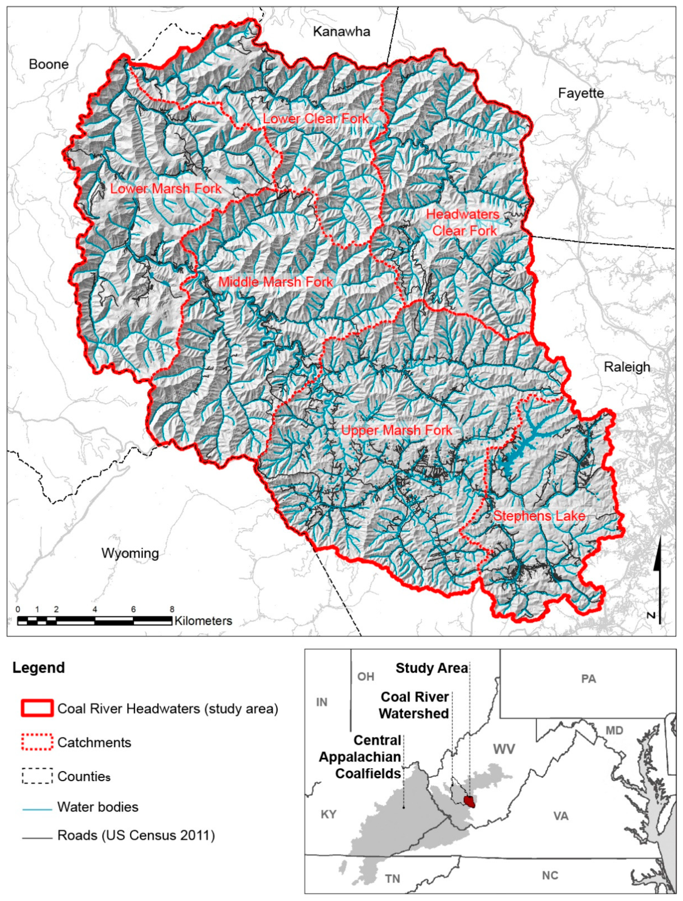
3.1. Study Area

The study area consists of 58,661 hectares of the Big Coal River’s headwaters in WV (USA), and includes the two main tributary branches: Clear Fork and Marsh Fork (Figure 3). The area is part of the Appalachian Plateau physiographic province, which is characterized by drainage networks with dendritic shapes, deeply incised and dissected valleys, steep slopes and a high degree of local relief, and narrow winding ridges [63]. The northern portion of the study area consists of the Clear Fork catchment and the Mash Fork basin’s lower and middle catchments. Land cover in this area is mainly characterized by forest and surface mining-related classes and MTRVF sites. In the valley floors, built-up areas, infrastructures, and industrial facilities used for coal processing, storage, and transport are frequent.

The southern part of the study area, consisting of the Upper Marsh Fork and Stephens Lake catchments, is a plateau with a noticeably different morphology than the rest of the study area. It has higher valley-bottom elevations but less local relief. Land cover in this part of the study area is dominated by open areas with grasslands and widespread settlements that densify to the East near the town of Beckley.

3.2. Data Collection and Processing

All the LCCs were based on a pre-processing geographic object-based image analysis (GEOBIA) phase [64,65]. The variables derived from the segmentation analyses, which included ancillary data from Landsat satellites and digital elevation model (DEM) derivatives, were processed using machine learning (ML) supervised classification algorithms in R [66]. The use of historical images in this study introduced further difficulties due to the lack of spectral information in the primary databases and the limitations of building a proper validation sample. Other difficulties arose from classifying specific LC classes, like the scattered settlements (developed areas) and the fine-grain, linear patterns characteristic of the strip mining operations (barren land). The 2016 LCC was obtained from an existing dataset of WV [44]. Each LCC included the error matrices and the number of samples derived from the validation polygons used during the classification stages. The study also included an intermediate post-processing phase conducted after the LCCs to reduce the amount of misclassified areas from the maps before the Intensity Analysis stage.

3.2.1. The LCC of 1976

For the 1976 LCC, three datasets were used during the classification process. The primary dataset consisted of an orthomosaic derived from 31 single black and white aerial photographs obtained from the U.S. Geological Survey (USGS) collected in 1976 and 1977. The high-resolution digital images (2 m) were derived from the original black-and-white (BW) panchromatic film (V-F Panchromatic) [67]. The 3 m DEM for the 1976 classification was produced from digital line graph (DLG) contour lines derived from 1:24,000 scale, 7.5 × 7.5 Minute Map Series Historical Topographic Maps that range from 1965 to 1969 [68]. The orthomosaic was obtained using the Imagine Photogrammetry add-on in Erdas Imagine v16.5 [69]. Ground points were derived from 1996 Digital Orthophoto Quarter Quads (DOQQs) [67] as a reference for X and Y coordinates using points with recognizable locations, such as streets intersections and buildings; the heights (Z coordinates) were derived from the 1965–1969 DEM included in the photogrammetric model. The final Total Image Unit-Weight root mean square error (RMSE) for the orthomosaic was equal to 0.89 (meters). Tonal and brightness differences were corrected using MosaicPro in Erdas Imagine. A Landsat 1 Multispectral Scanner (MSS) image from 1976 (June 7) with four spectral bands was obtained [68]. The band files were stacked to a single raster using the Layer Stack tool in ERDAS Imagine.

The 1976 LC included six classes and was derived with a 2-m resolution (

Table 1. The 1976 land cover classes definition.

Class Name	Description
Barren	Non-vegetated areas generally associated with surface mine features, strip-mining roads, spoil banks, coal deposits, dump sites.
Deciduous forest	Areas dominated by broad-leaved trees and woodlands.
Evergreen forest	Areas dominated by evergreen trees. It can include evergreen shrubs.
Low vegetation	Low vegetation areas such as grasslands, including pastureland, agricultural fields, pastures, and croplands.
Developed areas	Areas dominated by mixed development, residential areas and yards; areas characterized by impervious surface such as roads and parking lots. It can also include industrial complex and facilities used for coal processing.
Water	All waterbodies, including rivers, lakes, water ponds and coal sludge impoundments.

). The general method used for the LCCs of 1976 and 1996 was based on a pre-processing GEOBIA phase undertaken using eCognition [70]. Variables derived for each object during the segmentation analysis were provided as predictor variables for a ML supervised classification in R using the caret package [71] with the ranger method [72]. To potentially improve the classification performance, additional variables were obtained from the ancillary data (satellite image and topographic derivatives). The 1976 LCC was based on an unbalanced training dataset with 108 variables obtained with the multiresolution segmentation algorithm in eCognition. The validation sample was derived using a two-stage stratified cluster random sampling design [46,73]. The sampling design process consisted of generating random points throughout the study area extent; then, image objects intersecting these points were selected to create the validation set. The objects were assigned to the closest class by visual inspection of the 1976–1977 orthomosaic. The number of objects used for the training and validation samples are reported in Table S5.

The overall accuracy for the 1976 LCC was estimated at 95.0%.

Table 2. The error matrix for the classification of 1976. Values in the cells represent the number of objects, while accuracies are reported with the percentage of land area.

		Reference
		Barren	Deciduous Forest	Evergreen Forest	Low Vegetation	Developed Areas	Water	Row Tot.	User’s Accuracy % (Commission Errors)
Classification	Barren	131	1	0	0	1	0	133	98.5
	Deciduous forest	11	52	0	0	0	0	63	82.5
	Evergreen forest	0	0	66	0	0	0	66	100.0
	Low vegetation	0	2	0	54	1	0	57	94.7
	Developed areas	4	0	0	0	53	0	57	93.9
	Water	0	0	0	0	0	26	26	100.0
	Column tot.	146	55	66	54	55	26	Overall accuracy 95.0%
	Producer’s accuracy (%) (omission errors)	89.7	94.6	100.0	100.0	96.4	100.0

reports the error matrix for this classification with overall accuracy, user’s accuracy, and producer’s accuracy [52]. The error matrix obtained in Ranger (Table S2) was converted to an Estimated population Matrix using the PontiusMatrix42. Figure 4 reports the plots derived using PontiusMatrix42 [74], including the false alarm (commission or false positive) and miss (omission or false negative) components of error divided into the three parameters of Quantity, Exchange and Shift disagreement. PontiusMatrix42 allowed estimation and Comparison of the size of the errors to the size of the unbalanced samples used to validate the LCC [6].

The barren class obtained the lowest producer’s accuracy of 89.7%; it presented the largest miss quantity and exchange components. Confusion exists between this class and the deciduous forest and developed areas. Deciduous forest obtained the largest false alarm quantity. The low vegetation class tended to be overestimated; those errors were present, especially in plateau areas characterized by low slope values where the importance of the topographic variables, used in the classifier, decrease. The water class only captured main waterbodies since rivers were generally too narrow to be distinguished.

3.2.2. The LCC of 1996

Three datasets were used to derive the 1996 LC. The main dataset used for the segmentation analysis was a mosaic derived from 35 USGS color infrared (CIR) Digital Orthophoto Quadrangles (DOQs) collected in 1996. Digital images have a 1m resolution and three bands (G, R, NIR). The images were collected as part of the National Aerial Photography Program (NAPP) [67]. The final mosaic was assembled in Erdas Imagine v16.5, where overlapping areas, tonal, and brightness differences were adjusted using the MosaicPro tools. Additional spectral information was added using seven spectral bands obtained with the Landsat 5 Thematic Mapper (TM) on 18 September 1995 [68]. To derive elevation measures and DEM derivatives, the 2003 WV Statewide Addressing and Mapping Board (SAMB) photogrammetrically derived DEM was used [75], since it had the best temporal alignment with the imagery.

The 1996 LC was based on seven classes with a 1-m spatial resolution (

Table 3. The 1996 land cover classes definition.

Class Name	Description
Barren clear	Non-vegetated areas generally not associated with impervious surface. This class includes surface mine features and non-impervious roads.
Barren dark	Surface mining areas characterized by coal presence and large coal deposits.
Deciduous forest	Areas dominated by broad-leaved trees and woodlands.
Evergreen forest	Areas dominated by evergreen trees. It can include evergreen shrubs.
Low vegetation	Low vegetation areas such as grasslands, including pastureland, agricultural fields, pastures, and croplands.
Developed areas	It includes areas dominated by mixed development, residential areas and yards; areas characterized by impervious surface such as roads and parking lots. It can also include industrial complex generally used to process coal.
Water	All waterbodies, including rivers, lakes, water impoundments and coal sludge impoundments.

). It was obtained using the Ranger package in R with an unbalanced training dataset based on 139 variables derived with the multiresolution segmentation algorithm in eCognition, following the same method used in the LCC of 1976. The validation sample (Table S6) was obtained following the same procedures described in the classification of 1976, and by visual inspection of the aerial images of 1996. The overall accuracy was estimated at 87.3%.

Table 4. The error matrix for the classification of 1996. Values in the cells represent the number of objects, while accuracies are reported with the percentage of land area.

			Reference
		Barren Clear	Barren Dark	Deciduous Forest	Evergreen Forest	Low Vegetation	Developed Areas	Water	Row Tot.	User’s Accuracy % (Commission Errors)
Classification	Barren clear	40	0	0	0	1	9	0	50	80.0
	Barren dark	0	48	0	0	1	1	0	50	96.0
	Deciduous forest	2	0	41	5	1	1	0	50	82.0
	Evergreen forest	0	0	0	50	0	0	0	50	100.0
	Low vegetation	0	0	2	1	47	0	0	50	94.0
	Developed areas	6	0	0	0	0	40	1	47	85.1
	Water	0	9	0	0	0	1	40	50	80.0
	Column tot.	48	57	43	56	50	52	41	Overall accuracy 88.2%
	Producer’s accuracy (%) (omission errors)	83.3	84.2	95.4	89.3	94.0	76.9	97.6

reports the error matrix of the classification converted to an Estimated population Matrix using the PontiusMatrix42; Table S3 reports the error matrix obtained in Ranger. Figure 5 shows the miss and false alarm components of error derived with PontiusMatrix42. The lowest producer’s accuracy was obtained for the developed areas class, resulting from confusion with the barren clear class; overall, the class was underestimated, and misses were the prevalent source of error. Barren clear class presented false alarms, mostly due to confusion with developed areas (impervious surface) and deciduous forest (probably due to the presence of forest clear cuts). Another class that showed a relatively low producer’s accuracy was the barren dark class, due to a similar spectral signature with the water class, which included coal sludge impoundments. In the case of barren dark, omission errors were prevalent. In contrast, commission errors characterized the water class. The classifier overestimated the water class at the expense of barren dark and developed areas classes, especially in the flatter plateau areas where slope and curvature variables derived from the DEM had negligible effects.

3.2.3. The LCC of 2016

The classification of 2016 was derived from a high-resolution state LCC produced by the Natural Resource Analysis Center (NRAC) of WV University in 2018. It is based on the 2016 US Department of Agriculture National Agriculture Imagery Program (NAIP) orthophotography and DEM derivatives obtained from the 10 m USGS National Elevation Dataset (NED). The 2016 LCC has a 1-m resolution and six LC classes (

Table 5. The 2016 land cover classes definition.

Class Name	Description
Forest	Areas dominated by tall, woody vegetation and mature forests. This class includes forest and woodlands.
Low vegetation	Low vegetation such as grasslands, pastureland, agricultural fields, and croplands.
Barren	Non-vegetated areas not associated with impervious surface. This class includes bare soil, quarries, and surface mine features.
Water	All standing water, including rivers, streams, ponds, lakes, and impoundments.
Impervious surfaces	All areas dominated by impervious surface, such as road surfaces, parking lots, airport runways, and buildings.
Mixed developed	Areas dominated by mixed development and mixed land cover, such as residential areas, yards, and development.

). The methods used to obtain the LCC have been fully described in Maxwell et al. (2019) [44]. The sample size with the number of training and validation objects is reported in Table S7. The error matrix from Maxwell et al. (2019) [44] (Table S4) was converted to an Estimated population Matrix using the PontiusMatrix42 (

Table 6. The error matrix for the classification of 2016. Values in the cells represent the number of objects, while accuracies are reported with the percentage of land area.

		Reference
		Barren	Forest	Low Vegetation	Impervious	Mixed Developed	Water	Row Total	User’s Accuracy (Commission Errors)
Classification	Barren	66	4	36	52	1	4	163	40.5%
	Forest	11	19,826	532	49	131	13	20,562	96.4%
	Low vegetation	74	84	2873	35	80	0	3146	91.3%
	Impervious	18	5	31	318	31	22	425	74.8%
	Mixed developed	0	47	84	80	304	2	517	58.8%
	Water	1	18	4	1	1	163	188	86.7%
	Column total	170	19,984	3560	535	548	204	Overall Accuracy: 96.2%
	Producer’s accuracy (%) (omission errors)	38.8%	99.2%	80.7%	59.4%	55.5%	79.9%

). The classes that presented lower accuracies were barren, impervious, and developed areas. Confusion was reported between the barren and impervious classes and among the mixed developed, low vegetation and impervious classes. The plots obtained with the PontiusMatrix42 highlighted the false alarm quantity component for the forest class, while for the low vegetation (grass) reported large omission errors; for the mixed developed areas and barren classes, the exchange components, relating to miss quantities, appeared to be dominant (Table 6, Figure 6).

3.3. Study Area Land Cover Classifications Post-Processing Phase

A post-processing phase followed the LCCs [51]. It consisted of three separate steps: the first one concerned the optimization of the number of classes and resolution to allow their comparison during the change detection phase; the second phase focused on the LCCs of 1976 and 1996, where misclassified portions of the maps were extensively remapped; a final step involved overlaying some vector data to improve the quality of the LCCs.

3.3.1. Optimizing Land Cover Classes and Resolution

The three LCCs were aggregated into five classes (

Table 7. Description of the classes adopted in the three LCCs after the post-processing phase.

Class Name	Description
Forest	Areas dominated by trees and woodlands.
Low vegetation	Low vegetation areas such as grasslands, including pastureland, agricultural fields, pastures, and croplands.
Barren	Non-vegetated areas generally associated with surface mine features, strip-mining roads, spoil banks, coal deposits, dump sites.
Water	All waterbodies, including rivers, lakes, water impoundments and coal sludge impoundments.
Developed areas	Areas dominated by mixed development, residential areas, and yards; areas characterized by impervious surface such as roads and parking lots. Industrial facilities generally used for coal processing.

) to allow their comparison. In the 1976 LCC the number of classes was brought from 6 to 5, aggregating the deciduous forest and the evergreen forest classes. In the 1996 LCC, the number of classes was decreased from 7 to 5. The barren-clear class was combined with barren-dark, and the deciduous forest class was merged with the evergreen forest. In the 2016 LCC, the number of classes was decreased from 6 to 5; impervious and mixed developed classes were aggregated. All classes were aggregated and mapped following a consistent pattern to avoid inconsistencies among the portions of the maps.

3.3.2. Analyzing and Correcting the Misclassified Portions of the Maps

The error analysis derived by the category-level errors for the three LCCs (Table 2, Table 4 and Table 6, and Figure 4, Figure 5 and Figure 6) was followed by a visual inspection of the maps and correcting their obvious errors. The LCC maps were overlaid with their respective reference orthoimages to remove the most relevant misclassified areas; the areas misclassified by the ML algorithms were reallocated to the more appropriate LC class.

In the 1976 LCC, particular attention was given to removing the barren class omission. A large miss quantity for the barren class in the 1976 LCC corresponded to most of the false alarms reported for the deciduous forest class. Indeed, large exchange components may indicate systematic errors, like misclassification or misregistration, between a couple of categories [58]. Another category that was improved in the 1976 LCC was the low-vegetation class. It expressed a tendency to gain over the deciduous forest class; this happened mainly in the plateau’s relatively flat areas, where slope variables had limited importance in the classification.

In the 1996 LCC, errors between industrial areas and barren-dark and between barren-clear and developed areas classes were generally removed. Moreover, the water class in this classification tended to be overestimated (commission errors), especially in the plateau’s flat areas and in the presence of settlements in areas where the number of small impoundments was increased.

Water was consistently remapped in the three LCCs. As previous studies experienced, small water bodies in the region are difficult to map due to confusion with the shadows generated by the forest class [44].

The developed areas class in the three LCCs was subjected to limited editing. Due to the GEOBIA objects from which it was derived and the organization of the residential settlements in the area, this class presented an inherent confusion, particularly with the low-vegetation class. This inherent confusion was challenging to remove in the three LCCs. Moreover, in the study area, abandonment processes in which vegetation often gains on industrial settlement and built-up areas are not infrequent; they have also been documented by specific studies carried out in the area [16]. Therefore, we suggest that the transitions concerning the developed areas’ quantities should be considered with caution. They may contain suspected amounts of error that are difficult to assess when combined in multiple classifications. We will focus on this class more carefully in the results phase, using the framework proposed by [6] and accompanying the results’ discussion with the high-resolution aerial imagery’s visual assessment.

3.3.3. Overlaying Geospatial Data

A final phase consisted of overlaying the three LCCs with the same vector geospatial data representing rivers and lakes. This step was necessary to define, within the three-timepoints, the main water bodies characterized by no change. Indeed, while no relevant changes occurred in the main rivers during the 1976–2016 interval, considerable changes involved the water class, such as the numerous coal sludge impoundments realized for mining uses.

3.4. LCCs Sizes Comparison

Table 7 reports the five classes adopted in the three LCCs, while Figure 7 reports the three LCC maps after the post-processing phase and a histogram with LC class size comparisons. Table S8 reports the quantities of LC classes in the three LCCs after the post-processing phase.

3.5. Multi-Level Intensity Analysis and Difference Components

The intensity analysis relied on 1976, 1996, and 2016 LCCs obtained after the post-processing phase. The three LCCs identify two intervals of 20 years for a total range of 40 years. The two transition matrices [58], from 1976–1996 and 1996–2016, were obtained with the Land-Change Modeler (LCM) in TerrSet [76], the graphics used to describe land transitions were derived using the intensity.analysis R package [77]. The graphics showing the Difference Components of change (Quantity, Exchange, and Shift) were derived using PontiusMatrix42 and PontiusMatrix41 [78]. The maps showing gains and losses were derived using the crosstab raster generated with the LCM in TerrSet.

4. Results

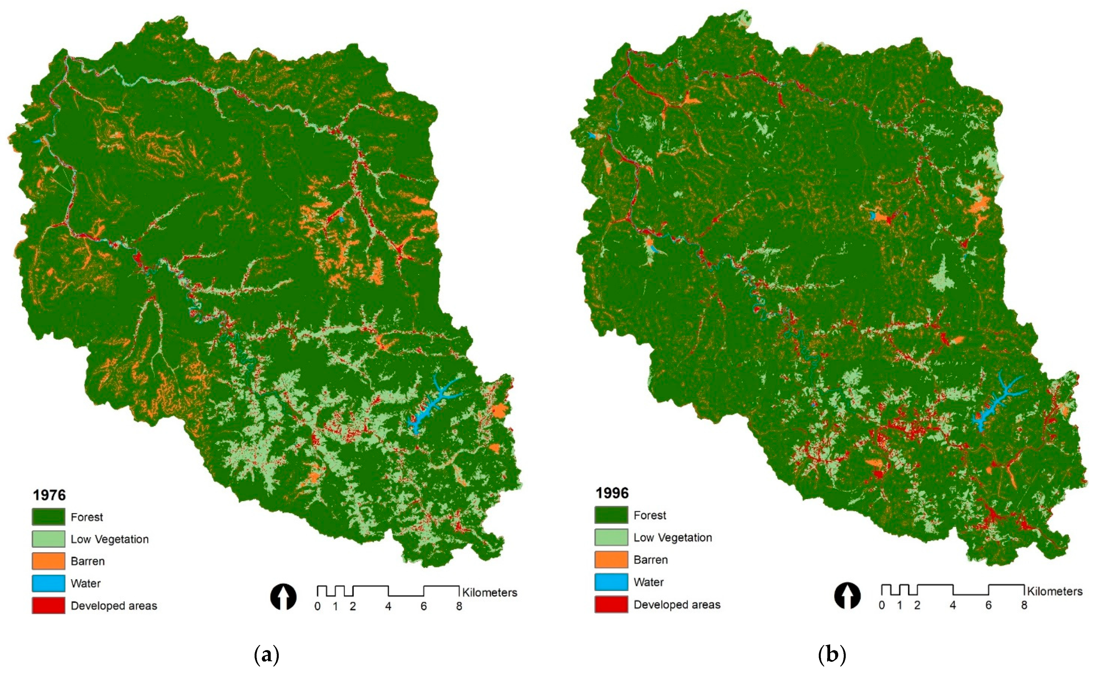
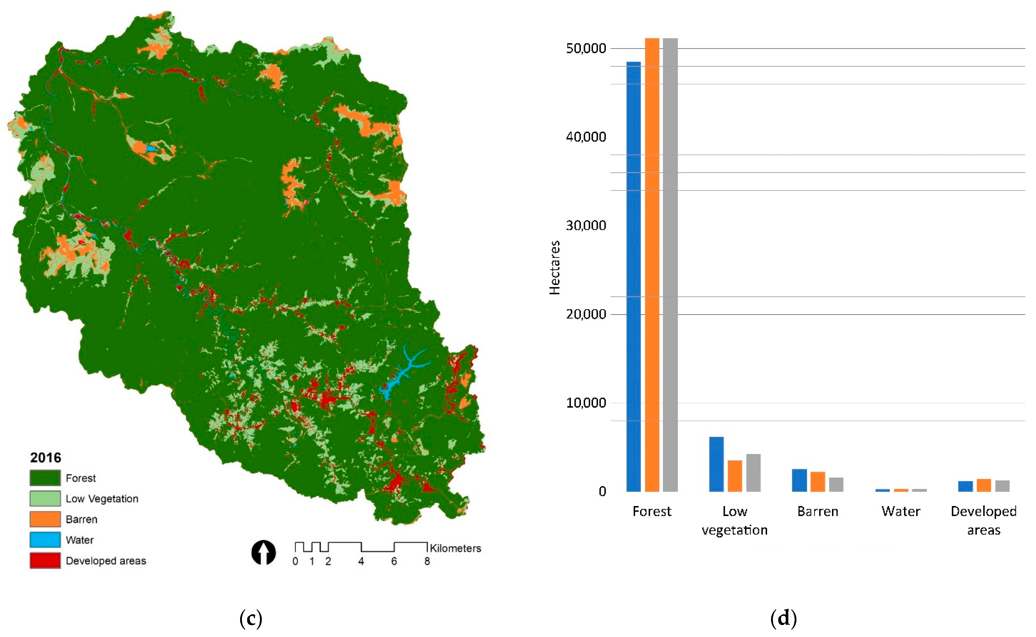
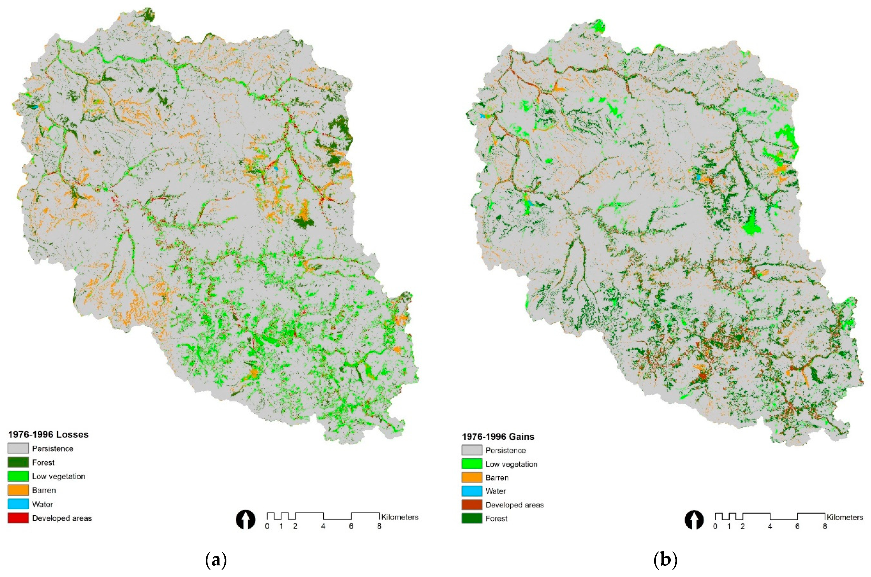
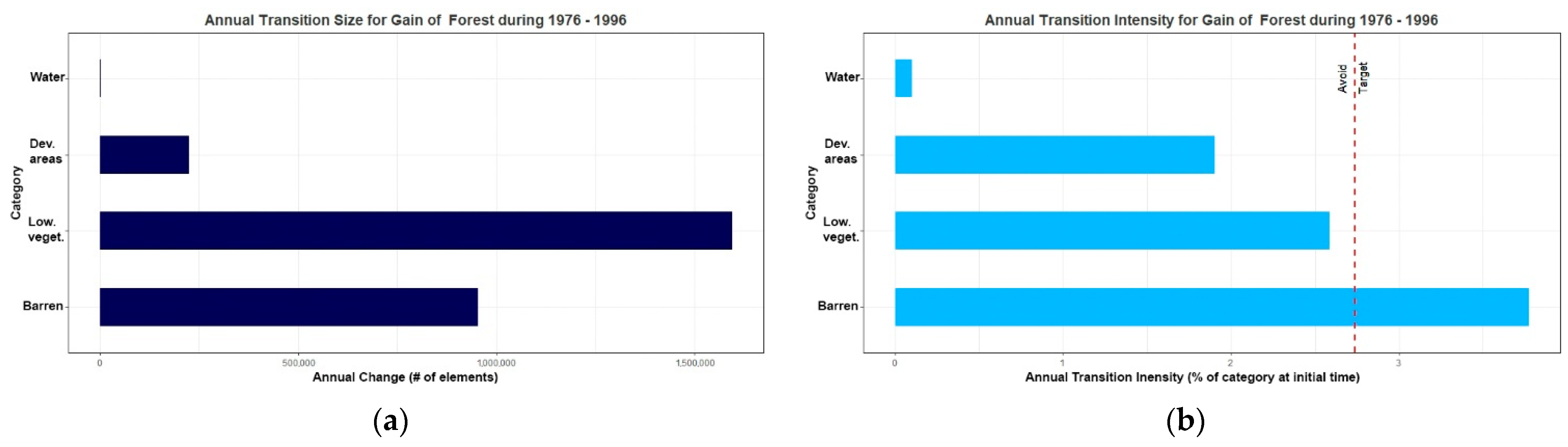
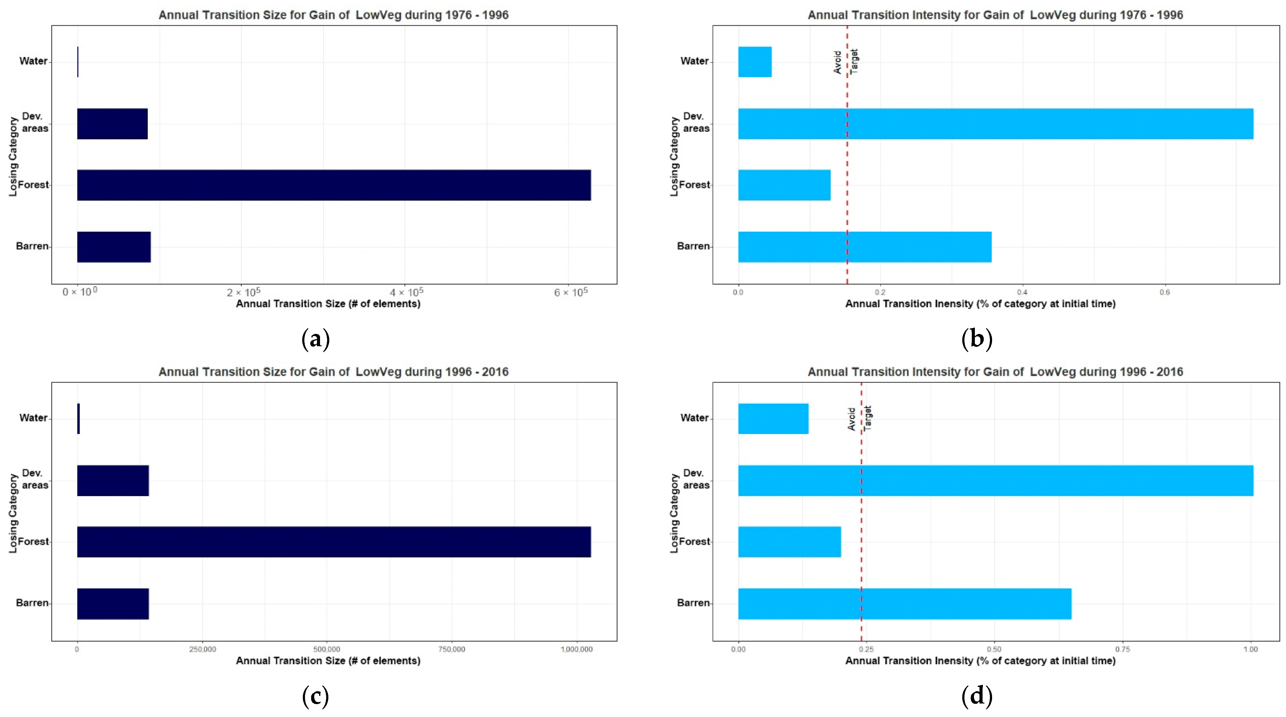
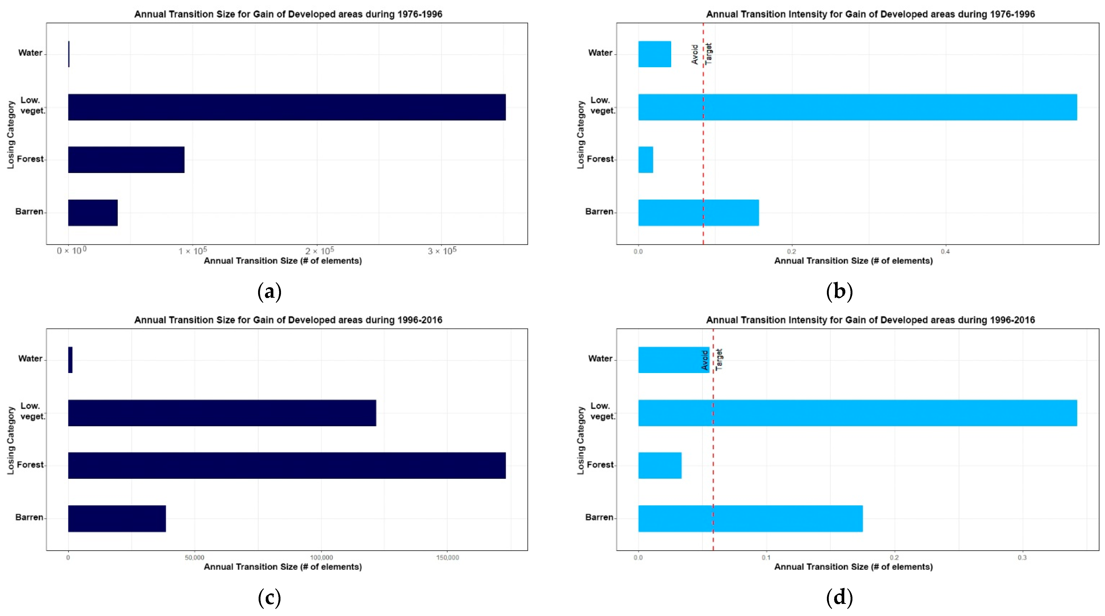
4.1. Land-Change and Multi-Level Intensity Analysis Results

The results of the two transition matrices, from 1976–1996 and 1996–2015, generated from the LCM in TerrSet are reported in

Table 8. The transition matrix of the Coal River head watershed from 1976 to 1996. Values are in hectares.

1996
		Forest	Low Vegetation	Barren	Water	Developed Areas	Total Cover (1976)	Gross Loss
1976	Forest	45,586.4	1255.4	1449.0	30.6	187.1	48,508.4	2922.0
	Low vegetation	3191.7	1945.1	305.2	15.8	704.0	6161.8	4216.7
	Barren	1910.8	180.4	350.5	11.1	79.6	2532.5	2182.0
	Water	5.6	2.6	3.9	259.7	2.3	274.1	14.4
	Developed areas	451.2	171.8	101.4	4.5	455.4	1184.3	728.9
	Total cover (1996)	51,145.8	3555.2	2209.9	321.8	1428.4		Total change
	Gross gain	5559.4	1610.1	1859.4	62.0	973.0		10063.9

and

Table 9. The transition matrix of the Coal River head watershed from 1996 to 2016. Values are in hectares.

2016
		Forest	Low Vegetation	Barren	Water	Developed Areas	Total Cover (1996)	Gross Loss
1996	Forest	47,452.0	2057.0	1259.6	31.8	346.2	51,145.8	3694.6
	Low vegetation	1578.4	1634.2	94.7	4.3	243.5	3555.2	1921.0
	Barren	1642.0	287.4	192.5	10.5	77.5	2209.9	2017.4
	Water	22.7	8.8	13.1	273.6	3.6	321.8	48.2
	Developed areas	476.4	287.5	40.8	5.3	618.4	1428.4	810.1
	Total cover (2016)	51,170.7	4275.0	1600.8	325.6	1289.2		Total change
	Gross gain	3719.5	2640.7	1408.3	52.0	670.8		8491.3

. The rows of the matrices show the classes for the first time point while the columns show the classes for the second time point. The transition matrix diagonal shows the persistence components, representing the areas that did not experience any change. The values off the diagonal correspond to transitions from one category into another. A row with gross loss and a column with gross gain were added in both matrices; those values show the total of row or column minus the persistence component. More details about calculation and matrix interpretation have been given in [60].

Table 10. Total Change, Net Change, and Swap values for the two intervals. Values are in hectares.

	1976–1996				1996–2016
	Gross Loss	Absolute Value of Net Change (Quantity Difference)	Total Change (Quantity Difference + Allocation Difference)	Swap (or Allocation Difference)	Gross Loss	Absolute Value of Net Change (Quantity Difference)	Total Change (Quantity Difference + Allocation Difference)	Swap (Allocation Difference)
Forest	2922.0	2637.4	8481.4	5844.0	3694.6	24.8	7414.1	7389.3
Low vegetation	4216.7	2606.6	5826.8	3220.1	1921.0	719.8	4561.7	3842.0
Barren	2182.0	322.6	4041.3	3718.8	2017.4	609.2	3425. 7	2816.5
Water	14.4	47.7	76.4	28.7	48.2	3.8	100.2	96.4
Developed areas	728.9	244.2	1701.9	1457.7	810.1	139.2	1480.9	1341.6
Total	10,063.9	5858.4	20,127.7	14,269.4	8491.3	1496.8	16,982.5	15,485.7
As percentage of the study area	17.2%				14.5%

shows the values of Gross Loss (the sum of gross loss and gross gains), Net change and Swap for the two intervals. Maps (Figure 8) show areas with persistence, gains and losses for the two time intervals.

At the first level of the intensity analysis, the interval level, it is possible to observe that the 1976–1996 interval presents the largest change magnitude, with the percent of interval’s domain equal to 17.2%, while 1996–2016 interval has a percentage of change equal to 14.5% of the domain (Figure 9). The change size represents the total amount of change for each interval, expressed as a percentage of the study area. The intensity analysis defines the annual change rate in 1976–1996 as relatively faster, while the annual change rate of 1996–2016 is relatively slower when compared to uniform (Figure 9). Overall processes of change at the interval level are not stationary since they have a different annual rate of change.

At the category level, the results were derived using the intensity.analysis package in R. Gain Intensity represents the annual intensity of gross gain (equation 3 in [5]). Loss Intensity is the annual intensity of gross loss (Equation (4) in [5]). The Uniform Category Intensity is the annual intensity of change (Equation (1) in [5]). Graphics (Figure 10) were obtained with the intensity.analysis package in R, except the graphics (Figure 11) that express Quantity, Exchange, and Shift components of change were obtained with the PontiusMatrix42.

At the category level, during the 1976–1996 interval, the largest gain is reported by forest, while the low vegetation class has the most extensive gross loss. Even though the forest category has the largest gross gain (5559.4 ha), forest is dormant in both loss and gain due to the class’s large domain dimension. The most intense change is expressed by the barren class, with loss size almost equal to the gain size. The substantial Exchange components in this class highlight swap processes among categories, pointing at the processes of reclamation of the strip-mining from barren to forest for the losses, and mostly to the new emerging MTR operations for the new gains. The developed areas class expresses an active behavior, with almost equal annual gains and losses. Even in this case, the Exchange component is the most extensive one, indicating that potential errors may characterize this class [58]. The low vegetation class is active, with the annual losses larger than the annual gains. The large Exchange quantities (Figure 11) highlight consistent substitution processes, but the class is characterized by a significative loss Quantity component. Finally, the latter category that expresses an active behavior in this interval is the water class; it is active only in terms of gain. It is worth remembering that the water category includes coal sludge impoundments, which overall number and size in the region considerably increased after SMCRA (1977).

During the second time interval, from 1996 to 2016, barren class, developed areas, low vegetation, and water classes confirmed their active behavior. Forest remains a dormant class even if it has the most considerable annual change in annual loss and annual gain. Forest maintains its constant growth trend, although the size of losses is greatly increased compared to the previous time interval, mainly due to the new MTR operations that occurred in this time interval. Low vegetation registered a considerable increase in terms of size, while the intensity of annual gains is larger than the annual losses. This behavior is the opposite of the one registered in the previous phase. This process can be attributed to the large new MTR operations, where the artificial grasslands emerge as an effect of the SMCRA reclamation processes. The barren class has the absolute highest annual change intensity, not only in this time interval but also when compared to the previous one, highlighting that very intense changes characterize this class. Its absolute size is diminished due to larger gross losses. The large exchange component indicates processes of substitution within this class are dominant in this time interval when compared to net quantity (Figure 11). The annual change intensity of the developed areas highlights intense processes of change associated with this class. Compared to the previous time interval, this class expresses a slight contraction in terms of size, with the annual loss size relatively larger than the annual gain. Moreover, processes of gain and loss are now less intense and with an opposite behavior. Overall Net Change reports that developed areas now appear to be shrinking after the relative growth registered in the previous interval, indicating an inverse trend that may be suspicious. Water has almost an equal balance in terms of loss and gain, very close to a uniform behavior, with a slightly positive annual gain change intensity. On the category level, gain and loss processes are stationary during both time intervals for all classes except water. The stationary processes occur when the behavior of gains and losses intensity, compared to the uniform line, is constant across the time intervals. Water class behavior in terms of loss is not stationary; in the first time interval, it has a dormant behavior, while in the second interval, it has an active behavior.

At the third level of the intensity analysis, the transition level, only the most noteworthy results have been reported to examine the gains of some classes and recognize classes targeted in both intervals. Some results were omitted since errors may affect the size of some categories and affect the analysis at this level.

The annual transition size for the forest gain in both intervals was mainly obtained at the expenses of grass and barren land (Figure 12). All the transitions are stationary. While forest targeted barren class in both time intervals, it avoided low vegetation, developed areas, and water. It is worthwhile to mention that even though the low vegetation class experienced large losses due to forest growth, it was not targeted by the forest class. On the contrary, barren land is targeted by forest in both time intervals. In the case of forest gaining from low vegetation, it appears as an avoiding pattern that can be attributable to an overall expansion of forest at the expense of the generally neighboring low vegetation class. While in the case of forest gaining from barren class, it can be attributed to the intentional reclamation processes that characterize the strip mining areas after 1977 (SMCRA) that were generally recolonized by forest.

In the case of the low vegetation class, during both time intervals, the size of the transitions from forest to low vegetation was the largest one. This process can be attributed to the new MTRVF operations concentrated in formerly forested mountain ridges, replaced by new artificial grasslands. Nevertheless, in both time intervals, the most targeted category by grass in terms of annual transition intensity was the developed areas (Figure 13), highlighting potential processes of abandoning. These results are nonetheless suspicious since the developed area class presents an inherent error component. It is difficult to define how much of this class was targeted because of abandonment processes and settlement reshaping or because the intrinsic confusion derived from the LCCs. Further investigations are possible by conducting visual comparisons of the high-resolution images.

During the first time interval, the developed areas gained mainly from low vegetation while, during the second time interval, they gained mostly from forest. In both time intervals, low vegetation was the most intensively targeted class. Intensity processes are stationary in both time intervals (Figure 14). The growth of settlement occurred mostly during the first time interval in the southern plateau areas characterized by low vegetation. This process is easily recognizable from the visual inspection of the high-resolution aerial images.

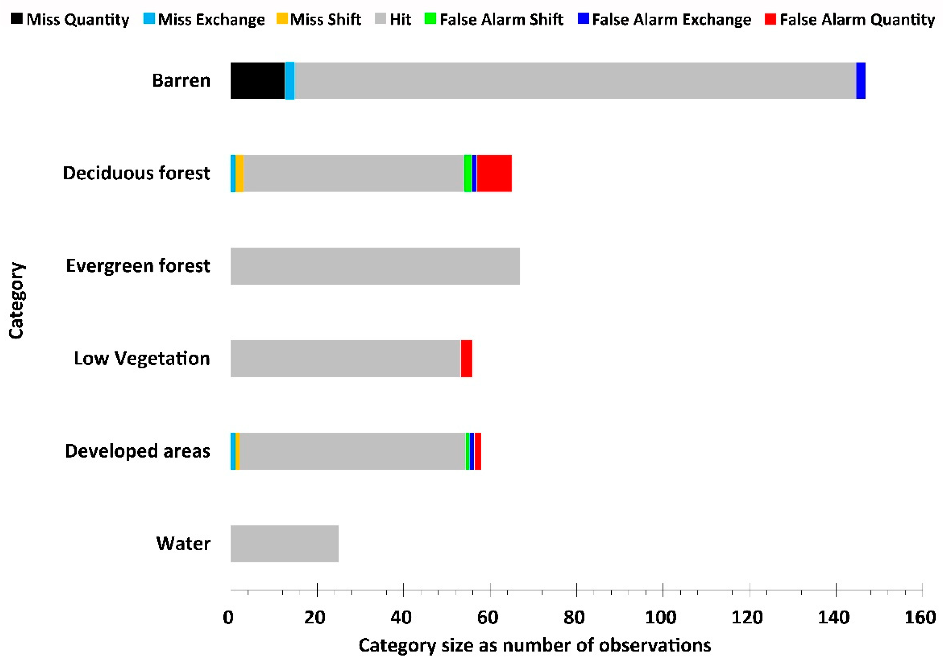
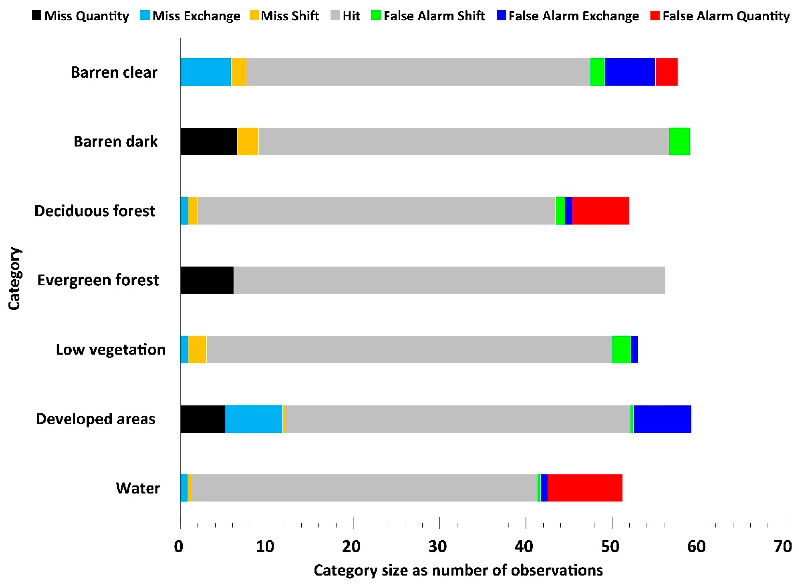
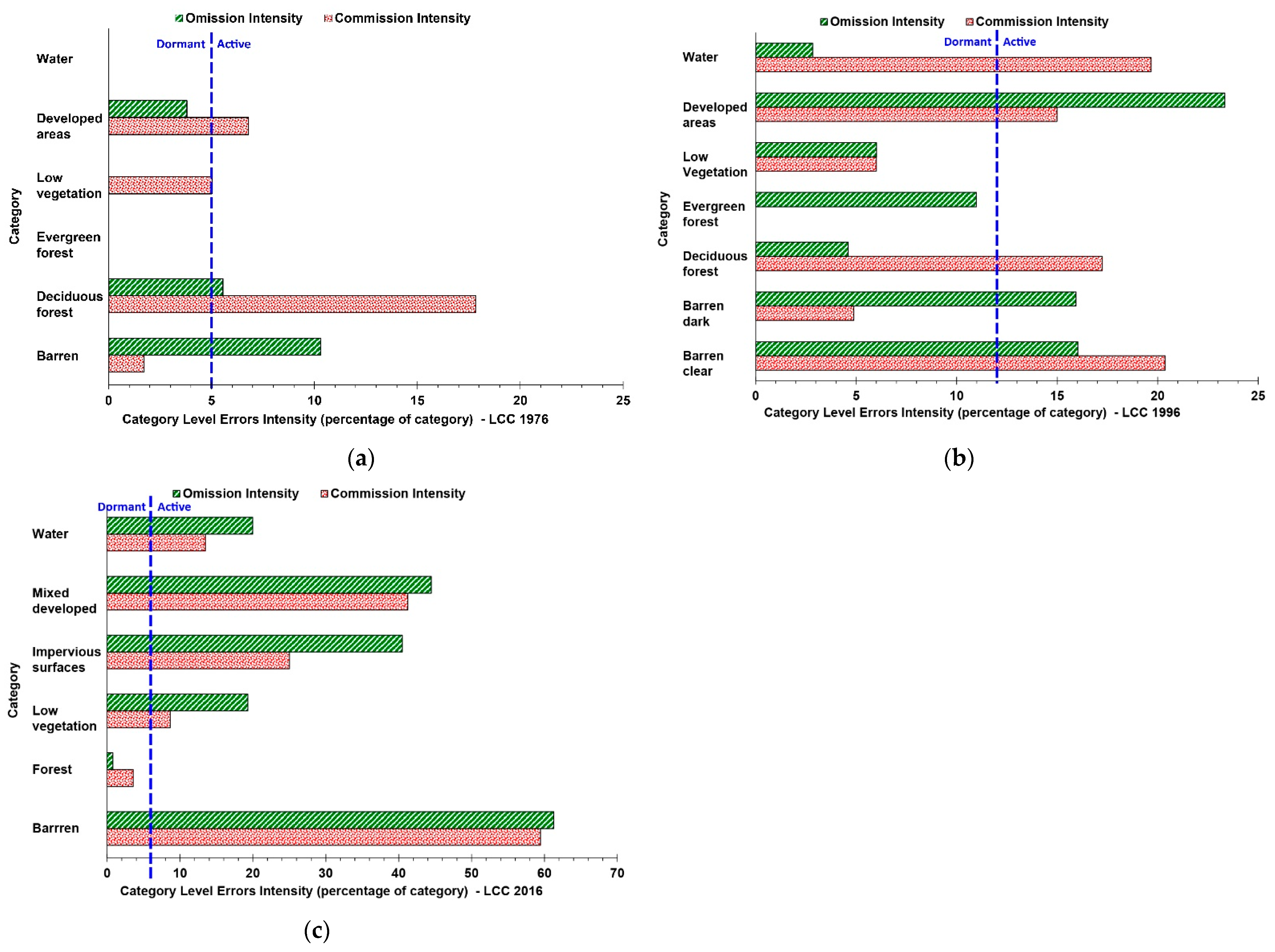
4.2. Land Change Errors Estimation

In land-change studies, errors emerge as a combined effect of the maps’ misclassified areas and may propagate when deriving the land change quantities [6,48,50,52]. In this study, due to the specific methods used, the LCCs’ errors may propagate due to several factors. Errors may derive from misregistration of the imagery, by errors derived from the segmentation analysis, and finally, by specific omission and commission errors produced by the classifiers.

In the case of image misregistration errors, we reported an RMSE relative to the 1976 orthomosaic equal to 0.89 m. As reported in Pontius (2019) [58], errors due to image misregistration are common and are generally reported in the Exchange component of change. Due to the scale of analysis and the multiple time-points used in the PCC, it is possible to assume that a component of this error is included in this study, even if the large size of the Exchange component can be considered as an effect of the land-change dynamics and not merely derived by errors.

In the case of GEOBIA, the segmentation phases generally produce objects that contain mismatches along the boundaries. Moreover, even if geo-objects are considered homogeneous, the polygons may include fuzziness [79]. In this study, this problem is more evident in the mixed developed class due to the character of settlement composition in the region, where a component of vegetation with trees or grasses is always present in the geo-objects. It was difficult to isolate and remove this error, even in the post-processing phase, due to its intrinsic characteristics.

Finally, other errors were derived from the supervised classification phase, where the classifier tended to reproduce commission and omission errors depending on the classification problem and the specific dataset. The errors derived from the classifiers were reported in the LCCs sections. Those errors were generally consistently removed in the post-processing phase, but still, some errors may persist.

The framework proposed by Xie et al. (2020) [6] compares the error size of the classifications to the size of change derived from the land-change study. We utilized this approach to estimate the developed areas class’s errors by comparing the land change quantities derived from the LCCs of 1976 and 1996 to the estimation derived from the land change results of 1976–1996. Indeed, we suspect that this class may include the largest quantity of errors concerning its size for the reasons above mentioned.

The size of temporal difference (total amount of change) between 1976 and 1996 is equal to 17.2% of the study area (Table 10). The 1976 LCC reported an overall error of around 5.0% (Table 2), while for the LCC of 1996, the overall error was equal to 11.8% (Table 4). Therefore, not all of the difference during the time interval 1976–1996 is real change. In the LCC of 1976, the developed areas class had user’s accuracy (commission) equal to 93.9% (commission error equal to 6.1%) and producer’s accuracy (omission) equal to 96.4% (omission error equal to 3.6%); the commission error was larger than the omission error, then the map overestimated this category. On the contrary, in the classification of the 1996 omission errors (23.1%) of the developed areas class was larger than commission error (14.9%). Therefore, the category was underestimated.

The gross gains in 1996 for the developed areas class were equal to 973 ha. The exchange component in the developed areas class during 1976–1996 (Figure 11d), which generally highlights most of the errors derived from misclassifications and misregistration [58], was equal to 882 ha. The difference between these two quantities indicates that even in the worst scenario where all the Exchange quantities were errors, the developed areas class during the interval 1976–1996 was gaining. Figure 15a–c reports the LCCs’ category level errors intensity before the post-processing phase and estimated as a percentage of the validation objects. Graphics were obtained with PontiusMatrix41; the uniform line in the figures represents the overall LCC error [6].

Nonetheless, it should be noted that the gaining of developed areas expresses the overall tendency of the class at the scale of the study area. It does not mean that, during this temporal interval, there was a uniform tendency of built-up areas in gaining across all the catchments of our study area; instead, we should expect opposite trends of contraction and expansion, but still, overall, the class experienced gain. In the LCC of 2016, developed areas were classified with relatively low accuracies (58.8% user’s accuracy and 55.5% of producer’s accuracy); therefore, we should expect that during the second time interval (1996–2016), there were more errors in land transitions that include this class. During 1996–2016, the developed areas reported gross loss larger than gross gains. It indicates built-up areas were shrinking; this inversion may point at potential abandonment processes that can be supported by the fact that low-vegetation targeted the developed class during this interval, as shown by the intensity analysis (Figure 13d). Nevertheless, the transitions are suspicious, even because of the large Exchange component, equal to 1268 ha (Figure 11d). More details about changes in this class are reported in the discussion sections, where inferences were derived from the observation of historical maps, LCCs, and high-resolution imagery.

5. Discussion

5.1. Methods

The method proposed in this study presented a complete framework based on a PCC approach to quantify relevant components of temporal land transitions. The method combined the use of LCCs based on high-resolution historical images with the framework of Intensity Analysis and Difference Components [6,58,80]. Except for limited examples [81], previous studies based on Intensity Analysis have generally grounded on low-resolution satellite images with few or no data about the LCCs error matrices [82,83,84,85,86,87,88].

The high-resolution images allowed us to collect the validation samples from the geospatial polygons derived from the segmentation analysis and assign them the best membership to the specific classes. This approach allowed us to obtain the error matrices for the LLCs of 1976 and 1996. The inclusion of the errors derived from the historical LCCs achieved in-depth information about errors propagation across the LC classes identifying the suspicious transitions within the land change analysis. Moreover, the PontiusMatrix42 allowed estimating false alarms and missing components of errors within each LCC. The inclusion of further ancillary datasets, like vector polygons, may be implemented within this method to improve the LCCs [44]. In the US, surface mining databases are being completed [89]; similar information can be obtained in other countries from historical maps or to apply this method to other LCC problems.

The integrated framework of Intensity Analysis and Difference Components, through a group of free and accessible tools, enables researchers to consider the components of errors and assess whether those errors may affect the results of the temporal analyses. The method makes it possible to exercise control over the error in land-change analysis based on PCC, encouraging the recognition of the more intense processes of change.

5.2. Landscape Transitions in the Coal River Headwaters

The findings revealed that the land change processes derived through the analysis of five relevant LC classes were not limited to surface mining sites and industrial facilities. Although coal mining has been the dominant driver of change in the region [7], its legacies on the landscape have interacted with other dynamics that are the outcome of previous and enduring socio-ecological processes.

Intensity analysis allowed us to compare the rate of change of the two time intervals (1976–1996, 1996–2016), showing us how, during the first interval, land-change processes were faster since they involved a larger percentage of change.

At the category level, forest class gained mainly during the first time interval with transitions characterized by different intensity levels. The barren class was continuously targeted by forest across the two intervals. A large part of this new forest grew over the former strip-mining barren areas; a process that is clearly distinguished by the LCCs and the high-resolution photographs. The intensity analysis highlights the non-uniform nature of this process, distinguishing it from a simple random event. The possible explanation identifies it as the outcome of intentional reclamation stages initiated before or after the SMCRA enactment. Limited information is available about the characteristic of these forested areas grown on barren mining land. In 1951 a USDA report [29] examined 105 plots in WV, describing the occurrence of natural tree and shrub species that generally spread out in the strip-mine spoils areas and above the overburdens. In those plots, black locusts were the most widespread trees, followed by red maples, black cherries, and sassafrasses. These reclamation processes were similar to those described by Townsend et al. (2009) [7] in areas where MTR never occurred.

During the first time interval, the low-vegetation class was the largest class from which forest gained, while during the second interval, it was the second larger one. Nevertheless, in both time intervals of the intensity analysis, the forest class did not target the low-vegetation class. Moreover, our results did not report any relevant forest growth within the surface mining permits of MTR operations [90]; these areas in the 2016 LCC are predominantly characterized by barren and low-vegetation classes.

During the first time interval (1976–1996), we observed an overall transition from barren to forest class that generally occurred on former strip-mining areas that were already mined in 1976–1977. During 1996, inside the permit boundaries, reclamation processes of former strip mining areas often occurred in conjunction with new surface minings. These new operations already presented the characters of the large surface mining operations typical of MTRVF, with dominant barren, low-vegetation, and water (sludge impoundments) classes. In the 2016 LCC, the areas characterized by MTRVF operations became much more considerable. The expansion of these areas occurred both on the predominantly undisturbed mountain ridges covered by forest and the former strip-mining areas characterized by ongoing reclamation processes and young trees. This study confirms that the areas characterized by former surface mines can be distinguished into at least two broad groups. The first group consists of the former strip-mining areas on which the forest class has apparently assumed stable characters; the second group is characterized mainly by MTRVF areas, which may overlap with previous mining operations. These operations are characterized by “remining” practices generally allowed because the reclamation was considered not completed [36]. Further considerations and in-depth studies could be based on more detailed information derived from the analysis of the mining permit boundaries since they generally present very articulated developments.

It is worth noting that the overall quantity of barren land from 1976 to 2016 diminished by approximately 37% in the study area. The loss of grasslands in the valley floors and the plateau was paradoxically compensated by the newly reclaimed areas, where novel ecosystems [91,92] characterized by poor topsoils spread with non-native and fast-growing grasses [93] emerged as outcome of the regulatory reclamation processes. Moreover, surface mines’ distribution changed from a spatially sprawled and more superficial one to a more compacted and deeper pattern. Recent studies based on DEMs measured the geological magnitude of these processes on a regional scale [23].

With regard to the general contraction of the low vegetated areas, it is worth noting that this process should not be directly ascribed only to coal mining. Indeed, it should probably be seen in continuity with the overall agricultural land abandonment processes reported in the Appalachian region at least from 1910 [94]. Among the variety of factors reported, the stagnation of farm productivity in Appalachia [15] and the decline of the traditional forest farming system [95] should be seen as those responsible for facilitating the introduction of new competitive practices of land use and the acquisition of land by the extractive industries of wood and coal.

The changes observed in the civilian and industrial settlements (the developed areas LC class) were articulated and followed fluctuating dynamics within the different sub-catchments of the study area. Even though this study presents some limitations due to the intrinsic fuzziness reported in classifying this category, it is worth reporting some patterns of changes in this class, because of the overall lack of studies conducted with similar methods in this region. The settlements’ dynamics of contraction and expansion in the area were mainly related to the economic cycles of growth and recession followed by the coal industry. During the interval 1880–1930, the first phase of rapid industrialization required labor to sustain the growth of coal industries [96]. Coal companies created several new towns in the Southern Appalachia, called company towns or coal towns. Following the mid-1920s, the coal industries bust contributed to the company towns’ progressive decline and, after the 1950s, to their definitive closure and dismantling [97]. During 1950–1970, WV lost 13% of the population [98]. The intensification of coal production regained strength after 1962, with the second phase of strip-mining intensification after 1970 [96]. Nevertheless, the population numbers in most old towns connected to the coal economy never regained the values reached during the first industrialization phase. Moreover, the intensification of surface mining operations led to consistent effects for the settlements located in the valley floors that experienced “the devastating externalities of coal mining” ([96], p. 28). As emerged from the intensity analysis, during both intervals (1976–1996 and 1996–2016), developed areas were the most targeted class by low vegetation. We already reported that this effect could be attributed to the fuzziness between low-vegetation and the developed areas class. Nevertheless, processes in which settlements were partially substituted by low vegetation class due to their abandonment or dismantlement have been recently documented in the study area [16]. In the lower catchments of the study area characterized by surface mining activities, we observed a pattern of settlement densification in the proximity of the most downstream areas. Settlement abandonment processes characterized the areas near the stream’s headwaters and closer to surface mining operations. On the contrary, in the plateau area, close to the town of Beckley, the developed areas class was characterized by a constant gain, with a more vigorous intensity during the first time interval. Here, the widespread phenomenon of suburbanization observed in the US and the more suitable landscape morphology may explain the processes of settlement intensification [99,100]. By way of example, the process of establishment and abandonment of the settlement of Montcoal during the interval 1912–2016 is reported in Figures S1 and S2 together with some detailed images derived from the LC maps. The settlement was established with the opening of a mine in Montcoal Mountain in 1916; it was one of the leading coal towns founded in the Coal River’s headwaters [96,97].

6. Conclusions

This article combined Intensity Analysis, Difference Components, and error analysis to assess land change processes applying a previous framework [6]. Additionally, this study provided three LCCs with accuracies assessments. The results confirm the method’s validity and reliability. Its application demonstrated that not all the temporal changes in the study area indicate actual landscape change. Moreover, the framework coupled with category accuracies from the historical classifications provided more in-depth details about how errors may propagate. The findings of this study allowed us to improve the characterization of the study area, deriving specific LC transitions and classes, like those described for the reclamation processes, and improving previous limited information about the land change processes before and after the SMCRA enactment in the region in 1977. Our study detected that the extent of disturbed land by surface mining in the study area increased by 38.9% compared to previous research.

The combined framework of Intensity Analysis and Difference Components allowed us to isolate and discuss suspicious transitions. A further step to the proposed approach, to produce a more complete framework, would be to integrate an additional error assessment phase following the LCCs post-processing. This would help to further detail all suspicious transitions and provide a more comprehensive quantitative assessment after the post-processing phase, which, although improved the overall accuracy, introduced an additional degree of indeterminacy. In addition, we suggest that given the multiplicity of co-occurring land-change dynamics and drivers generally present in the landscape, further analyses should include the comparison of different regions, catchments, or watersheds, to derive specific trends of growth or shrinkage and aggregate statistics using different spatial zones; some studies used this method using Intensity Analysis [81,84].

Information derived by land change studies can be of great importance for natural resource managers and future planning phases. It allows the characterization of large areas and the definition of historic-based and spatially explicit datasets. These data can inform models that can assess or readdress the efficacy of specific policies and inform conservation and natural resource management. In addition, assessing the analysis of the response produced by the socio-technological [101,102] reclamation practices can help in analyzing possible institutional failures or the achievements of specific policies [103].

Our study confirms the importance of land-change studies based on high-resolution and spatially explicit datasets. Indeed, detailed spatial scales of analysis may disclose details about overall landscape dynamics that characterize large regions. In the case presented, anthropogenic processes profoundly influenced the environmental and ecological dynamics of the study area, including relevant changes in ecosystem services provision, carbon sequestration, soil degradation, hydrologic cycles, water quality, habitat integrity, and biodiversity loss [104,105]. The study demonstrated the importance of site-specific studies and land-change analyses when dealing with deeply altered and fragile landscapes where human-based drivers, and not only the environmental gradients, have been responsible for changes that profoundly altered the landscape, its morphology, and the ecosystem structure and composition.

References

1. Griffith, M.B.; Norton, S.B.; Alexander, L.C.; Pollard, A.I.; Le Duc, S.D. The effects of mountaintop mines and valley fills on the physicochemical quality of stream ecosystems in the central Appalachians: A review. Sci. Total Environ. 2012, 417, 1–12. [Google Scholar] [CrossRef]
2. U.S. EPA. Draft Programmatic Environmental Impact Statement on Mountaintop Mining/Valley Fills in Appalachia; Region 3; U.S. Environmental Protection Agency: Philadelphia, PA, USA, 2003.
3. Maxwell, A.E.; Strager, M.P.; Yuill, C.B.; Petty, J.T. Modeling critical forest habitat in the southern coal fields of West Virginia. Int. J. Ecol. 2012, 2012, 182683. [Google Scholar] [CrossRef] [Green Version]
4. Rindfuss, R.; Entwisle, B.; Walsh, S.; Li, A.; Badenoch, N.; Brown, D.; Deadman, P.; Evans, T.; Fox, J.; Geoghegan, J.; et al. Land use change: Complexity and comparisons. J. Land Use Sci. 2008, 3, 1–10. [Google Scholar] [CrossRef] [Green Version]
5. Aldwaik, S.Z.; Pontius, R.G. Intensity analysis to unify measurements of size and stationarity of land changes by interval, category, and transition. Landsc. Urban. Plan. 2012, 106, 103–114. [Google Scholar] [CrossRef]
6. Xie, Z.; Pontius, R.G.; Huang, J.; Nitivattananon, V. Enhanced intensity analysis to quantify categorical change and to identify suspicious land transitions: A case study of Nanchang, China. Remote Sens. 2020, 12, 3323. [Google Scholar] [CrossRef]
7. Townsend, P.A.; Helmers, D.P.; Kingdon, C.C.; McNeil, B.E.; de Beurs, K.M.; Eshleman, K.N. Changes in the extent of surface mining and reclamation in the Central Appalachians detected using a 1976–2006 Landsat time series. Remote Sens. Environ. 2009, 113, 62–72. [Google Scholar] [CrossRef]
8. Turner, M.G.; Gardner, R.H. Landscape Ecology in Theory and Practice; Springer: New York, NY, USA, 2015; ISBN 9781493927937. [Google Scholar]
9. Farina, A. Landscape Dynamics. Available online: https://www.oxfordbibliographies.com/view/document/obo-9780199830060/obo-9780199830060-0182.xml (accessed on 24 May 2021).
10. Clarkson, R.B. Tumult on the Mountains: Lumbering in West Virginia 1770–1920; McClain Printing Company: Parson, WV, USA, 1964. [Google Scholar]
11. Eller, R.D. Miners, Millhands, and Mountaineers: Industrialization of the Appalachian South, 1880–1930; Twentieth-century America series; University of Tennessee Press: Knoxville, TN, USA, 1982. [Google Scholar]
12. Eller, R.D. Land as Commodity: Industrialization of the Appalachian Forests, 1880–1940. In The Great Forest: An Appalachian Story; Appalachian State University: Boone, UC, USA, 1985. [Google Scholar]
13. Davis, D.E. Where There Are Mountains An. Environmental History of the Southern Appalachians; The University of Georgia Press: Athens, GA, USA, 2000; ISBN 9788578110796. [Google Scholar]
14. Delcourt, P.A.; Delcourt, H.R. Prehistoric Native Americans and Ecological Change: Human Ecosystems in Eastern North America Since the Pleistocene; Cambridge University Press: Cambridge, UK, 2004; ISBN 9780521662703. [Google Scholar]
15. Marley, B.J. The Coal Crisis in Appalachia: Agrarian Transformation, Commodity Frontiers and the Geographies of Capital. J. Agrar. Chang. 2016, 16, 225–254. [Google Scholar] [CrossRef]
16. Staniscia, S.; Yuill, C.; Cribari, V. Four plus one dimensions of transferability: Defining a framework for the application of a landscape characterization in the USA. City Territ. Archit. 2020, 7, 8. [Google Scholar] [CrossRef]
17. Pericak, A.A.; Thomas, C.J.; Kroodsma, D.A.; Wasson, M.F.; Ross, M.R.V.; Clinton, N.E.; Campagna, D.J.; Franklin, Y.; Bernhardt, E.S.; Amos, J.F. Mapping the yearly extent of surface coal mining in Central Appalachia using Landsat and Google Earth Engine. PLoS ONE 2018, 13, e0197758. [Google Scholar] [CrossRef] [Green Version]
18. Drummond, M.A.; Loveland, T.R. Land-use Pressure and a Transition to Forest-cover Loss in the Eastern United States. Biosci. TA 2010, 60, 286–298. [Google Scholar] [CrossRef]
19. Brown, D.G.; Johnson, K.M.; Loveland, T.R.; Theobald, D.M. Rural Land-Use Trends in the Conterminous United States, 1950–2000. Ecol. Appl. 2005, 15, 1851–1863. [Google Scholar] [CrossRef] [Green Version]
20. Hendryx, M. Mortality from heart, respiratory, and kidney disease in coal mining areas of Appalachia. Int. Arch. Occup. Environ. Health 2009, 82, 243–249. [Google Scholar] [CrossRef] [PubMed]
21. Palmer, M.A.; Bernhardt, E.S.; Schlesinger, W.H.; Eshleman, K.N.; Foufoula-Georgiou, E.; Hendryx, M.S.; Lemly, A.D.; Likens, G.E.; Loucks, O.L.; Power, M.E.; et al. Mountaintop Mining Consequences: Damage to ecosystems and threats to human health and the lack of effective mitigation require new approaches to mining regulation. Science 2010, 327, 148–149. [Google Scholar] [CrossRef] [Green Version]
22. Wickham, J.; Wood, P.B.; Nicholson, M.C.; Jenkins, W.; Druckenbrod, D.; Suter, G.W.; Strager, M.P.; Mazzarella, C.; Galloway, W.; Amos, J. The Overlooked Terrestrial Impacts of Mountaintop Mining. Bioscience 2013, 63, 335–348. [Google Scholar] [CrossRef]
23. Ross, M.R.V.; McGlynn, B.L.; Bernhardt, E.S. Deep Impact: Effects of Mountaintop Mining on Surface Topography, Bedrock Structure, and Downstream Waters. Environ. Sci. Technol. 2016, 50, 2064–2074. [Google Scholar] [CrossRef] [PubMed] [Green Version]
24. KGS Coal Mining. Available online: http://www.uky.edu/KGS/coal/coal-mining.php# (accessed on 21 November 2018).
25. Montrie, C. Expedient Environmentalism: Opposition to Coal Surface Mining in Appalachia and the United Mine Workers of America, 1945–1975. Environ. Hist. 2000, 5, 75–98. [Google Scholar] [CrossRef]
26. Eggleston, J.R. Newsletter of West Virginia Geological and Economic Survey; West Virginia Geological and Economic Survey: Morgantown, WV, USA, 1975; pp. 23–33.
27. Murphy, R.E. Wartime changes in the patterns of united states coal production. Ann. Assoc. Am. Geogr. 1947, 37, 185–196. [Google Scholar] [CrossRef]
28. Fishman, L.; Fishman, B.G. Bituminous Coal Production during World War II. South. Econ. J. 1952, 18, 391–396. [Google Scholar] [CrossRef]
29. USDA. Refeorestation of Strip-Mined Lands in West Virginia; USDA: Washington, DC, USA, 1951.
30. Austin, R.C.; Borrelli, P. The Strip Mining of America: An Analysis of Surface Coal Mining and the Environment; Sierra Club: New York, NY, USA, 1971. [Google Scholar]
31. McGinley, P. From Pick and Shovel to Mountaintop Removal: Environmental Injustice in The Applachian Coalfields. Environ. Law 2004, 34, 21–106. [Google Scholar]
32. Zipper, C.E.; Lee Daniels, W.; Bell, J.C. The Practice of ”Approximate Original Contour” in the Central Appalachians. II. Economic and Environmental Consequences of an Alternative. Landsc. Urban. Plan. 1989, 18, 139–152. [Google Scholar] [CrossRef]
33. West Virginia Division of Culture and History Buffalo Creek Disaster. Available online: http://www.wvculture.org/history/buffcreek/bctitle.html (accessed on 24 May 2021).
34. Wes Virginia Dump Sites Survey. Identification and Photographs: Coal Refuse Dumps of West Virginia; West Virginia Department of Natural Resources: South Charleston, WV, USA, 1972.
35. Holl, K. Primer of Ecological Restoration; Island Press: Washington, DC, USA, 2020; ISBN 1559633123. [Google Scholar]
36. Dicks, N.; Simpson, M.; Bingaman, J. Surface Coal Mining: Characteristics of Mining in Mountainous Areas of Kentucky and West Virginia; DIANE Publishing: Collingdale, PA, USA, 2009. [Google Scholar]
37. Skousen, J.; Zipper, C.E. Post-mining policies and practices in the Eastern USA coal region. Int. J. Coal Sci. Technol. 2014, 1, 135–151. [Google Scholar] [CrossRef] [Green Version]
38. Zipper, C.E.; Skousen, J. (Eds.) Appalachia’ s Coal-Mined Landscapes. Resources and Communities in a New Energy Era; Springer: New York, NY, USA, 2021; ISBN 9783030577797. [Google Scholar]
39. Evans, B.M.; Kern, J.R.; Stingelin, R.W. Low Altitude Photointerpretation Manual for Surface Coal Mining Operations; Office of Surface Mining Reclamation and Enforcement: Washington, DC, USA, 1983.
40. Slonecker, E.T.; Benger, M.J. Remote sensing and mountaintop mining. Remote Sens. Rev. 2001, 20, 293–322. [Google Scholar] [CrossRef]
41. Simmons, J.A.; Currie, W.S.; Eshleman, K.N.; Kuers, K.; Monteleone, S.; Negley, T.L.; Pohlad, B.R.; Thomas, C.L. Forest to reclaimed mine land use change leads to altered ecosystem structure and function. Ecol. Appl. 2008, 18, 104–118. [Google Scholar] [CrossRef]
42. Maxwell, A.E.; Warner, T.A. Differentiating mine-reclaimed grasslands from spectrally similar land cover using terrain variables and object-based machine learning classification. Int. J. Remote Sens. 2015, 36, 4384–4410. [Google Scholar] [CrossRef] [Green Version]
43. Maxwell, A.E.; Warner, T.A.; Vanderbilt, B.C.; Ramezan, C.A. Land cover classification and feature extraction from National Agriculture Imagery Program (NAIP) Orthoimagery: A review. Photogramm. Eng. Remote Sens. 2017, 83, 737–747. [Google Scholar] [CrossRef]
44. Maxwell, A.E.; Strager, M.P.; Warner, T.A.; Ramezan, C.A.; Morgan, A.N.; Pauley, C.E. Large-area, high spatial resolution land cover mapping using random forests, GEOBIA, and NAIP orthophotography: Findings and recommendations. Remote Sens. 2019, 11, 1409. [Google Scholar] [CrossRef] [Green Version]
45. Warner, T.; Almutairi, A.; Lee, J. Remote sensing of land cover change. In The SAGE Handbook of Remote Sensing; Warner, T.A., Nellis, M.D., Foody, G.M., Eds.; SAGE Publications Ltd.: London, UK, 2009; pp. 459–472. [Google Scholar]
46. Jensen, J.R. Introductory Digital Image Processing: A Remote Sensing Perspective; Prentice Hall Press: Hoboken, NJ, USA, 2015. [Google Scholar]
47. Lu, D.; Mausel, P.; Brondízio, E.; Moran, E. Change detection techniques. Int. J. Remote Sens. 2004, 25, 2365–2407. [Google Scholar] [CrossRef]
48. Pontius, R.G.; Lippitt, C.D. Can error explain map differences over time? Cartogr. Geogr. Inf. Sci. 2006, 33, 159–171. [Google Scholar] [CrossRef]
49. Fuller, R.M.; Smith, G.M.; Devereux, B.J. The characterisation and measurement of land cover change through remote sensing: Problems in operational applications? Int. J. Appl. Earth Obs. Geoinf. 2003, 243–253. [Google Scholar] [CrossRef]
50. Olofsson, P.; Foody, G.M.; Herold, M.; Stehman, S.V.; Woodcock, C.E.; Wulder, M.A. Good practices for estimating area and assessing accuracy of land change. Remote Sens. Environ. 2014, 148, 42–57. [Google Scholar] [CrossRef]
51. Van Oort, P.A.J. Interpreting the change detection error matrix. Remote Sens. Environ. 2007, 108, 1–8. [Google Scholar] [CrossRef]
52. Olofsson, P.; Foody, G.M.; Stehman, S.V.; Woodcock, C.E. Making better use of accuracy data in land change studies: Estimating accuracy and area and quantifying uncertainty using stratified estimation. Remote Sens. Environ. 2013, 129, 122–131. [Google Scholar] [CrossRef]
53. Aldwaik, S.Z.; Pontius, R.G. Map errors that could account for deviations from a uniform intensity of land change. Int. J. Geogr. Inf. Sci. 2013, 27, 1717–1739. [Google Scholar] [CrossRef]
54. Braimoh, A.K. Random and systematic land-cover transitions in northern Ghana. Agric. Ecosyst. Environ. 2006, 113, 254–263. [Google Scholar] [CrossRef]
55. Shoyama, K.; Braimoh, A.K. Analyzing about sixty years of land-cover change and associated landscape fragmentation in Shiretoko Peninsula, Northern Japan. Landsc. Urban. Plan. 2011, 101, 22–29. [Google Scholar] [CrossRef]
56. Alo, C.A.; Pontius, R.G. Identifying systematic land-cover transitions using remote sensing and GIS: The fate of forests inside and outside protected areas of Southwestern Ghana. Environ. Plan. B Plan. Des. 2008, 35, 280–295. [Google Scholar] [CrossRef]
57. Meyfroidt, P. Approaches and terminology for causal analysis in land systems science. J. Land Use Sci. 2016, 11, 501–522. [Google Scholar] [CrossRef]
58. Pontius, R.G. Component intensities to relate difference by category with difference overall. Int. J. Appl. Earth Obs. Geoinf. 2019, 46, 1. [Google Scholar] [CrossRef]
59. Pontius, R.G.; Santacruz, A. Quantity, exchange, and shift components of difference in a square contingency table. Int. J. Remote Sens. 2014, 35, 7543–7554. [Google Scholar] [CrossRef]
60. Pontius, R.G.; Shusas, E.; McEachern, M. Detecting important categorical land changes while accounting for persistence. Agric. Ecosyst. Environ. 2004, 101, 251–268. [Google Scholar] [CrossRef]
61. Pickard, B.; Gray, J.; Meentemeyer, R. Comparing quantity, allocation and configuration accuracy of multiple land change models. Land 2017, 6, 52. [Google Scholar] [CrossRef] [Green Version]
62. Pontius, R.G.; Millones, M. Death to Kappa: Birth of quantity disagreement and allocation disagreement for accuracy assessment. Int. J. Remote Sens. 2011, 32, 4407–4429. [Google Scholar] [CrossRef]
63. Ehlke, T.A.; Runner, G.S.; Downs, S.C. Hydrology of Area 9, Eastern Coal Province; US Department of the Interior: Washington, DC, USA, 1982.
64. Hay, G.J.; Castilla, G. Geographic object-based image analysis (GEOBIA). In Object-Based Image Analysis—Spatial Concepts for Knowledge-Driven Remote Sensing Applications; Blaschke, T., Lang, S., Hay, G.J., Eds.; Springer: Berlin, Germany, 2008; pp. 77–92. [Google Scholar]
65. Blaschke, T. Object based image analysis for remote sensing. ISPRS J. Photogramm. Remote Sens. 2010, 65, 2–16. [Google Scholar] [CrossRef] [Green Version]
66. R Core Team. R: A Language and Environment for Statistical Computing; R Core Team: Vienna, Austria, 2020. [Google Scholar]
67. USGS EROS Archive. Available online: https://www.usgs.gov/centers/eros/science/usgs-eros-archive-aerial-photography-aerial-photo-single-frames?qt-science_center_objects=0#qt-science_center_objects (accessed on 25 May 2021).
68. USGS EarthExplorer. Available online: https://earthexplorer.usgs.gov/ (accessed on 25 May 2021).
69. Hexagon Geospatial Erdas Imagine; v16.5; Erdas Inc.: Madison, AL, USA, 2018.
70. Trimble eCognition Developer; v9.3; Trimble Geospatial: Sunnyvale, CA, USA, 2019.
71. Kuhn, M. Building Predictive Models in R Using the caret Package. J. Stat. Softw. 2008, 28, 647–673. [Google Scholar] [CrossRef] [Green Version]
72. Wright, M.N.; Ziegler, A. ranger: A Fast Implementation of Random Forests for High Dimensional Data in C++ and R. J. Stat. Softw. 2017, 77, 1–17. [Google Scholar] [CrossRef] [Green Version]
73. Stehman, S.V. Sampling designs for accuracy assessment of land cover. Int. J. Remote Sens. 2009, 30, 5243–5272. [Google Scholar] [CrossRef]
74. Pontius, R.G., Jr. PontiusMatrix, V.42. 2020. Available online: www.clarku.edu/~rpontius (accessed on 25 May 2021).
75. USGS and SAMB West Virginia Statewide Digital Elevation Models. Available online: https://wvgis.wvu.edu/data/dataset.php?ID=261 (accessed on 25 May 2021).
76. TerrSet: Geospatial Monitoring and Modeling Software; v18.31; Clark Labs, Clark University: Worcester, MA, USA, 2017.
77. Pontius, R.G., Jr.; Khallaghi, S. Package ‘Intensity Analysis’, v0.1.6. 2019. Available online: https://cran.r-project.org/web/packages/intensity.analysis/index.html (accessed on 25 May 2021).
78. Pontius, R.G., Jr. PontiusMatrix, V.41. 2018. Available online: www.clarku.edu/~rpontius (accessed on 25 May 2021).
79. Radoux, J.; Bogaert, P. Good practices for object-based accuracy assessment. Remote Sens. 2017, 9, 646. [Google Scholar] [CrossRef] [Green Version]
80. Shafizadeh-Moghadam, H.; Minaei, M.; Feng, Y.; Pontius, R.G. GlobeLand30 maps show four times larger gross than net land change from 2000 to 2010 in Asia. Int. J. Appl. Earth Obs. Geoinf. 2019, 78, 240–248. [Google Scholar] [CrossRef]
81. Mallinis, G.; Koutsias, N.; Arianoutsou, M. Monitoring land use/land cover transformations from 1945 to 2007 in two peri-urban mountainous areas of Athens metropolitan area, Greece. Sci. Total Environ. 2014, 490, 262–278. [Google Scholar] [CrossRef]
82. Enaruvbe, G.O.; Pontius, R.G. Influence of classification errors on Intensity Analysis of land changes in southern Nigeria. Int. J. Remote Sens. 2015, 36, 244–261. [Google Scholar] [CrossRef]
83. Pontius, R.G.; Li, X. Land transition estimates from erroneous maps. J. Land Use Sci. 2010, 5, 31–44. [Google Scholar] [CrossRef]
84. Quan, B.; Pontius, R.G.; Song, H. Intensity Analysis to communicate land change during three time intervals in two regions of Quanzhou City, China. GISci. Remote Sens. 2019, 57, 21–36. [Google Scholar] [CrossRef]
85. Huang, B.; Huang, J.; Gilmore Pontius, R.; Tu, Z. Comparison of Intensity Analysis and the land use dynamic degrees to measure land changes outside versus inside the coastal zone of Longhai, China. Ecol. Indic. 2018, 89, 336–347. [Google Scholar] [CrossRef]
86. Shoyama, K.; Braimoh, A.K.; Avtar, R.; Saito, O. Land Transition and Intensity Analysis of Cropland Expansion in Northern Ghana. Environ. Manag. 2018, 62, 892–905. [Google Scholar] [CrossRef] [PubMed]
87. Akinyemi, F.O.; Pontius, R.G.; Braimoh, A.K. Land change dynamics: Insights from Intensity Analysis applied to an African emerging city. J. Spat. Sci. 2017, 62, 69–83. [Google Scholar] [CrossRef]
88. Huang, J.; Pontius, R.G.; Li, Q.; Zhang, Y. Use of intensity analysis to link patterns with processes of land change from 1986 to 2007 in a coastal watershed of southeast China. Appl. Geogr. 2012, 34, 371–384. [Google Scholar] [CrossRef]
89. Horton, J.D.; San Juan, C.A. Prospect- and Mine-Related Features from U.S. Geological Survey 7.5- and 15-Minute Topographic Quadrangle Maps of the United States; Ver. 6.0, April 2021; U.S. Geological Survey: Reston, VA, USA, 2021.
90. (DMR) Permit Boundary. Available online: https://tagis.dep.wv.gov/site/GISData (accessed on 21 April 2021).
91. Hobbs, R.J.; Higgs, E.; Hall, C.M.; Bridgewater, P.; Chapin, F.S.; Ellis, E.C.; Ewel, J.J.; Hallett, L.M.; Harris, J.; Hulvey, K.B.; et al. Managing the whole landscape: Historical, hybrid, and novel ecosystems TT. Front. Ecol. Environ. 2014, 12, 557–564. [Google Scholar] [CrossRef] [Green Version]
92. Higgs, E. Novel and designed ecosystems. Restor. Ecol. 2017, 25, 8–13. [Google Scholar] [CrossRef]
93. Bauman, J.M.; Cochran, C.; Chapman, J.; Gilland, K. Plant community development following restoration treatments on a legacy reclaimed mine site. Ecol. Eng. 2015, 83, 521–528. [Google Scholar] [CrossRef]
94. Hart, J.F. Loss and Abandonment of Cleared Farm Land in the Eastern United States. Ann. Assoc. Am. Geogr. 1968, 417–440. [Google Scholar] [CrossRef]
95. Otto, J.S. The Decline of Forest Farming in Southern Appalachia. J. For. Hist. 1983, 27, 18–27. [Google Scholar] [CrossRef]
96. Hufford, M. Landscape and History at the Headwaters of the Big Coal River Valley: An Overview. In Tending the Commons: Folklife and Landscape in Southern West Virginia; The Library of Congress: Washington, DC, USA, 2007. [Google Scholar]
97. Shifflett, C.A. Coal Towns. Life, Work, and Culture in Company Towns of Southern Appalachia, 1880–1960; The University of Tennessee Press: Knoxville, TN, USA, 1991. [Google Scholar]
98. Pollard, K.M. Population Growth and Distribution in Appalachia: New Realities; Appalachian Regional Commission: Washington, DC, USA, 2005.
99. Jackson, K.T. Crabgrass Frontier: The Suburbanization of the United States; Oxford University Press: New York, NY, USA, 1985. [Google Scholar]
100. Beauregard, R. When America Became Suburban; University of Minnesota Press: Minneapolis, MN, USA, 2006. [Google Scholar]
101. Geels, F.W. Technological transitions as evolutionary reconfiguration processes: A multi-level perspective and a case-study. Res. Policy 2002, 31, 1257–1274. [Google Scholar] [CrossRef] [Green Version]
102. Ahlborg, H.; Ruiz-Mercado, I.; Molander, S.; Masera, O. Bringing technology into social-ecological systems research-Motivations for a socio-technical-ecological systems approach. Sustainability 2019, 11, 2009. [Google Scholar] [CrossRef] [Green Version]
103. Ostrom, E. Governing the Commons: The Evolution of Institutions for Collective Action; Cambridge University Press: Cambridge, UK, 1990. [Google Scholar]
104. Daily, G.C. Nature’s Services: Societal Dependence on Natural Ecosystems; Island Press: Washington, DC, USA, 1997; ISBN 1597267759. [Google Scholar]
105. Qiu, J.; Queiroz, C.; Bennett, E.M.; Cord, A.F.; Crouzat, E.; Lavorel, S.; Maes, J.; Meacham, M.; Norström, A.V.; Peterson, G.D.; et al. Land-use intensity mediates ecosystem service tradeoffs across regional social-ecological systems. Ecosyst. People 2021, 17, 264–278. [Google Scholar] [CrossRef]
Figure 1. Effects of surface minings and highwall mining in the Appalachian landscape in 1972: (a) dump site number 129, Boone County, WV [34]; (b) dump site number 253, Wyoming County, WV [34]. (c) MTRVF reclaimed landscape: Kayford Mountain, WV, 2018 (photo V. Cribari).
Land 10 00748 g001
Figure 2. Comparison of aerial views of the same area in 1976–1977 and 2016. After 40 years of vegetation growth, strip mining effects can be barely distinguished from the aerial images. Images are representative of the scale of surface mining operations that occurred in the area before the 1977. The site number 253 (Figure 1b) is highlighted in the red circle in both images. (a) Map derived from the orthomosaic used for the land cover classification of 1976. (b) Map is based on the USDA National Agriculture Imagery Program (NAIP) 2016 dataset.
Land 10 00748 g002
Figure 3. Map of the study area.
Land 10 00748 g003
Figure 4. Category size errors for 1976. Miss and false alarm as number of observations.
Land 10 00748 g004
Figure 5. Category size errors for 1996. Miss and false alarm as number of observations.
Land 10 00748 g005
Figure 6. Category size errors for 2016. Miss and false alarm as number of observations.
Land 10 00748 g006
Figure 7. The three land cover classifications after the post-processing phase: (a) 1976; (b) 1996; (c) 2016; (d) land covers quantities plot for 1976, 1996, 2016. Values are in hectares.
Land 10 00748 g007aLand 10 00748 g007b
Figure 8. Maps show areas of gains and losses for each LC class during the two time intervals: (a) areas of losses from 1976–1996; (b) areas of gains from 1976–1996; (c) areas of losses from 1996–2016; (d) areas of gains from 1996–2016.
Land 10 00748 g008aLand 10 00748 g008b
Figure 9. Time interval change intensity (annual change %).
Land 10 00748 g009
Figure 10. Plots at the category level for the two intervals; (a) annual change size by category during 1976–1996; (b) annual change intensity by category during 1976–1996; (c) annual change size by category during 1996–2016; (d) annual change intensity by category during 1996–2016.
Land 10 00748 g010
Figure 11. (a) Category size changes 1976–1996; (b) difference size changes 1976–1996; (c) category size changes 1996–2016; (d) difference size changes 1996–2016. Sizes are in ha.
Land 10 00748 g011
Figure 12. Annual gain transitions of forest class during 1976–1996 and 1996–2016; (a) annual transition size for gain of forest during 1976–1996; (b) annual transition intensity for gain of forest during 1976–1996; (c) annual transition size for gain of forest during 1996–2016; (d) annual transition intensity for gain of forest during 1996–2016.
Land 10 00748 g012aLand 10 00748 g012b
Figure 13. Annual gain transitions of low vegetation class during 1976–1996 and 1996–2016; (a) annual transition size for gain of low vegetation during 1976–1996; (b) annual transition intensity for gain of low vegetation during 1976–1996; (c) annual transition size for gain of low vegetation during 1996–2016; (d) annual transition intensity for gain of low vegetation during 1996–2016.
Land 10 00748 g013
Figure 14. Annual gain transitions of developed areas class during 1976–1996 and 1996–2016; (a) annual transition size for gain of developed areas during 1976–1996; (b) annual transition intensity for gain of developed areas during 1976–1996; (c) annual transition size for gain of developed areas during 1996–2016; (d) annual transition intensity for gain of developed areas during 1996–2016.
Land 10 00748 g014
Figure 15. Category level errors intensity for the LCCs of 1976 (a), 1996 (b), 2016 (c).
Land 10 00748 g015