Integrating Spatial Markov Chains and Geographically Weighted Regression-Based Cellular Automata to Simulate Urban Agglomeration Growth: A Case Study of the Guangdong–Hong Kong–Macao Greater Bay Area

Abstract

Urban agglomeration is an important spatial organization mode in China’s attempts to attain an advanced (mature) stage of urbanization, and to understand its consequences, accurate simulation scenarios are needed. Compared to traditional urban growth simulations, which operate on the scale of a single city, urban agglomeration considers interactions among multiple cities. In this study, we combined a spatial Markov chain (SMC) (a quantitative composition module) with geographically weighted regression-based cellular automata (GWRCA) (a spatial allocation module) to predict urban growth in the Guangdong–Hong Kong–Macao Greater Bay Area (GBA), an internationally important urban agglomeration in southern China. The SMC method improves on the traditional Markov chain technique by taking into account the interaction and influence between each city to predict growth quantitatively, whereas the geographically weighted regression (GWR) gives an empirical estimate of urban growth suitability based on geospatial differentiation on the scale of an urban agglomeration. Using the SMC model to forecast growth in the GBA in the year 2050, our results indicated that the rate of smaller cities will increase, while that of larger cities will slow down. The coastal belt in the core areas of the GBA as well as the region’s peripheral cities are most likely to be areas of development by 2050, while established cities such as Shenzhen and Dongguan will no longer experience rapid expansion. Compared with traditional simulation models, the SMC-GWRCA was able to consider spatiotemporal interactions among cities when forecasting changes to a large region like the GBA. This study put forward a development scenario for the GBA for 2050 on the scale of an urban agglomeration to provide a more credible scenario for spatial planning. It also provided evidence in support of using integrated SMC-GWRCA models, which, we maintain, offer a more efficient approach for simulating urban agglomeration development than do traditional methods.

1. Introduction

Recent decades have seen a period of rapid urbanization, particularly in developing countries such as China [1,2,3], but the urban sprawl that results from economic and explosive population growth poses serious challenges to sustainable development [4,5,6,7]. Urbanization, regardless of country or region, has historically tended to follow a pattern: it accelerates at a rate of approximately 20%, slows down when it reaches around 60%, and stabilizes between 70 and 80% [8]. China’s National Bureau of Statistics noted that in 2020 the rate had exceeded 60% [9]. When urbanization entered a mature stage, China adopted an organizational model based on the spatial structure of the urban agglomeration to promote high-quality development [10,11,12]. Within this context, models that can simulate growth scenarios are needed; therefore, research into such models has the potential to constitute an important aid to policymakers for promoting sustainable urbanization [13].

A broad spectrum of simulation models has been developed to provide insight into dynamic urban growth scenarios [14,15]. Usually, these contain two modules: one dedicated to quantitative composition and one to address spatial allocation. The former focuses on analyzing changes in quantitative land use, while the latter focuses on analyzing the evolution of spatial patterns [16,17]. While the quantity of land-use change is mainly determined by the development of regional economies and social conditions, the spatial pattern is largely dependent on location conditions [18]. For example, undertaking residential and industrial development requires a supply of land, but that is determined by spatial factors such as terrain and transportation. Because quantitative land-use demand and the corresponding spatial pattern of land use are both determined by these two driving mechanisms, modelers often need to include coupling models. [19,20,21].

Previous studies have used a range of different methods to perform quantitative predictions of urban growth. The quantitative demand module in such models is often calculated by means of an independent external model such as the Markov chain (MC) [22,23,24,25,26], or system dynamics (SD) [27,28,29]. The latter model considers interactions between land-use change and social and economic development and can predict land-use demand in complex situations [30]. However, it first needs to abstract land-use and socioeconomic development into several independent subsystems and then establish the input and feedback mechanisms that link them [31,32]. Although SD can accurately reflect the complex mechanisms in land-use change, it has several important limitations: subsystem abstraction requires a high level of modeling experience, and model calibration requires a large number of historical or empirical parameters [33,34]. The trend interpolation approach (one alternative to the system dynamics model) has similar limitations in that it needs long-term sequential observational data to establish a change curve. In contrast to these two methods, the Markov chain model is able to predict changes in land-use structure based only on the land-use transfer probability. For this reason, the Markov chain method is widely used to predict the size of urban growth [35,36,37].

Usually, Markov chain models are constructed for a single city, so there are obvious risks in employing it on the scale of an urban agglomeration because the development of each city is quite different [38,39]. Consequently, a feasible measure is to establish a Markov process for an agglomeration can be described as a “spatial Markov chain” (SMC) [40,41]. Using this approach to estimate changes in land use entails more than simply building a Markov model for each city. While each city does require its own independent Markov process, the interaction and influence between urban agglomerations must also be considered [42,43] because land-use changes in a given city may be driven by forces exerted by surrounding cities [44,45]. In addition, the process must also be calibrated to reflect a given city’s level of urbanization and unique resource and environmental constraints, such as China’s “red line” policy, which seeks to ensure ecological security and basic farmland protection, limits the growth of some cities [46,47].

Although the quantitative composition module of an urban growth simulation is very important, an additional module is required to predict the spatial pattern of corresponding land-use changes. The basic allocation module uses either spatial probability, cellular automata (CA), or agent-based modeling (ABM) [48,49]. Among these, an allocation model based mainly on an evaluation of urban growth suitability constitutes the prototype for almost all other spatial allocation models [50]. By assuming that the growth of a city can be described probabilistically, the modeler can, for instance, employ a series of spatial factors (terrain, traffic conditions, distance from existing cities) to estimate the probability of urban sprawl [51,52]. The estimation algorithms include logistic regression [53]; decision trees [54], support vector machines [55], random forest techniques [56], and, more recently, deep learning neural networks [57]. Although the performance of these algorithms is different, they all mine the sample data to obtain the required parameters to estimate suitability. Despite its advantages, though, spatial probability-based allocation models have natural defects [14,15]. For example, if an insufficient number of change samples is collected during model estimation, the developmental probability of a region with ostensibly high potential can be seriously underestimated [58]. Once a spatial allocation model has determined an area’s probability, it tends to remain relatively unchanged, and that can cause researchers to miss dynamic effects [18]. This phenomenon is contrary to the findings of many observational studies that suggest that a region can drive the development of surrounding areas once it has reached a developed state. If neighborhood interaction is to be considered, the simulation framework must be able to discretize the whole into individuals, and the model to do this is cellular automata (CA) [48,59], at present the most widely used bottom-up model for simulating urban pattern evolution [49].

In general, the CA model focuses on analyzing spatial dynamic processes, while its counterpart, ABM, focuses more on analyzing the spatial movement of subjects [48]. For land-use change simulation, CA and ABM do not differ significantly from one another, so because this study focuses on the spatial pattern change of urban growth rather than an analysis of land-use change resulting from a particular socioeconomic behavior, we mainly used the CA model. As mentioned above, the essence of the CA approach is to consider neighborhood interaction based on an estimation of spatial probability, and estimating the spatial probability of urban sprawl was the key aim of the CA modeling in this study. The estimation was conducted in the same manner as using a traditional spatial probability allocation model. Whether researchers used the most advanced deep-learning neural network or the most classical logistic regression method to address the scale simulation of an urban agglomeration, the characteristics of geographic differentiation always had to be considered. Therefore, because historical change cannot fully account for a city’s future development and since even the best parameter-fitting method will only fit a historical process [60], this study used classical logistic regression to estimate the probability of urban sprawl together with a geographically weighted regression to calibrate cellular automata (GWRCA) because of the urban agglomeration’s varied geographical characteristics [61].

As discussed previously, the SMC model predicts land-use change while taking into account interactions between the cities in a network, while the GWRCA simulates large-scale urban growth. However, no model has so far been developed that can integrate the SMC and GWRCA methods to simulate dynamic urban agglomeration development despite the fact that agglomerations are cited as an important spatial structure for promoting China’s further urbanization. Therefore, this study presents a model framework that couples the SMC and GWRCA techniques, thereby allowing researchers to simulate the development of urban agglomerations more realistically. The remainder of this article is organized according to the following structure. In Section 2, the study area and the dataset for model implementation are introduced. In Section 3, the steps and methods employed in building the model are discussed in detail. Section 4 presents the results and a discussion of the model implementation to validate the proposed urban CA model in simulating urban growth. Finally, the conclusions are presented in Section 5.

2. Materials and Methods

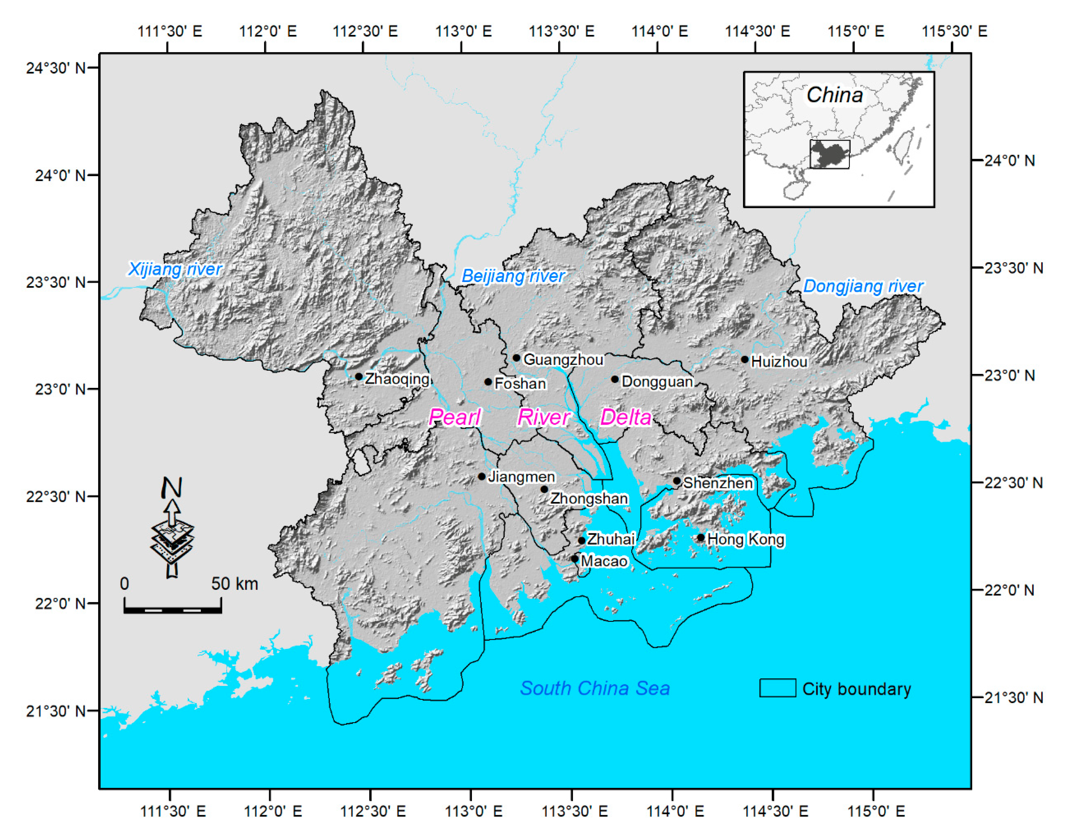
2.1. Study Area

Extending over a total area of 56,000 km², the Guangdong–Hong Kong–Macao Greater Bay Area (GBA) is composed of two Special Administrative Regions (Hong Kong (HK) and Macao (MO)) and nine cities in Guangdong Province (Guangzhou (GZ), Shenzhen (SZ), Zhuhai (ZH), Foshan (FS), Huizhou (HZ), Dongguan (DG), Zhongshan (ZS), Jiangmen (JM) and Zhaoqing (ZQ)) (Figure 1). At the end of 2020, the GBA had a total population of over 70 million and a GDP in excess of 10 trillion CNY. The GBA is located in south-central China, on a delta in the Pearl River Estuary formed by the accumulation of sediment from the Xijiang, Beijiang, and Dongjiang rivers and their tributaries. The western, northern, and eastern parts of the GBA are surrounded by hills and mountains, which form a natural barrier, and the southern boundary is a long coastline with many islands. The GBA is the fourth largest bay area in the world after those in New York, San Francisco, and Tokyo. It is also one of China’s most dynamic urban agglomerations [43]. The Chinese government requires that by 2050, the modernization level and the capacity of the land and space governance system be improved holistically to form a territory of “intensive and efficient production”; “livable and comfortable living space”; “beautiful ecological space”; and “safe, harmonious, competitive, and sustainable development” [62]. With that aim in mind, this study took 2050 as the target year to reveal the spatial pattern of the GBA through an SMC-GWRCA coupled simulation model, thereby specifying an urban spatial boundary to optimize the GBA infrastructure network.

2.2. Data for Urban Growth Simulation

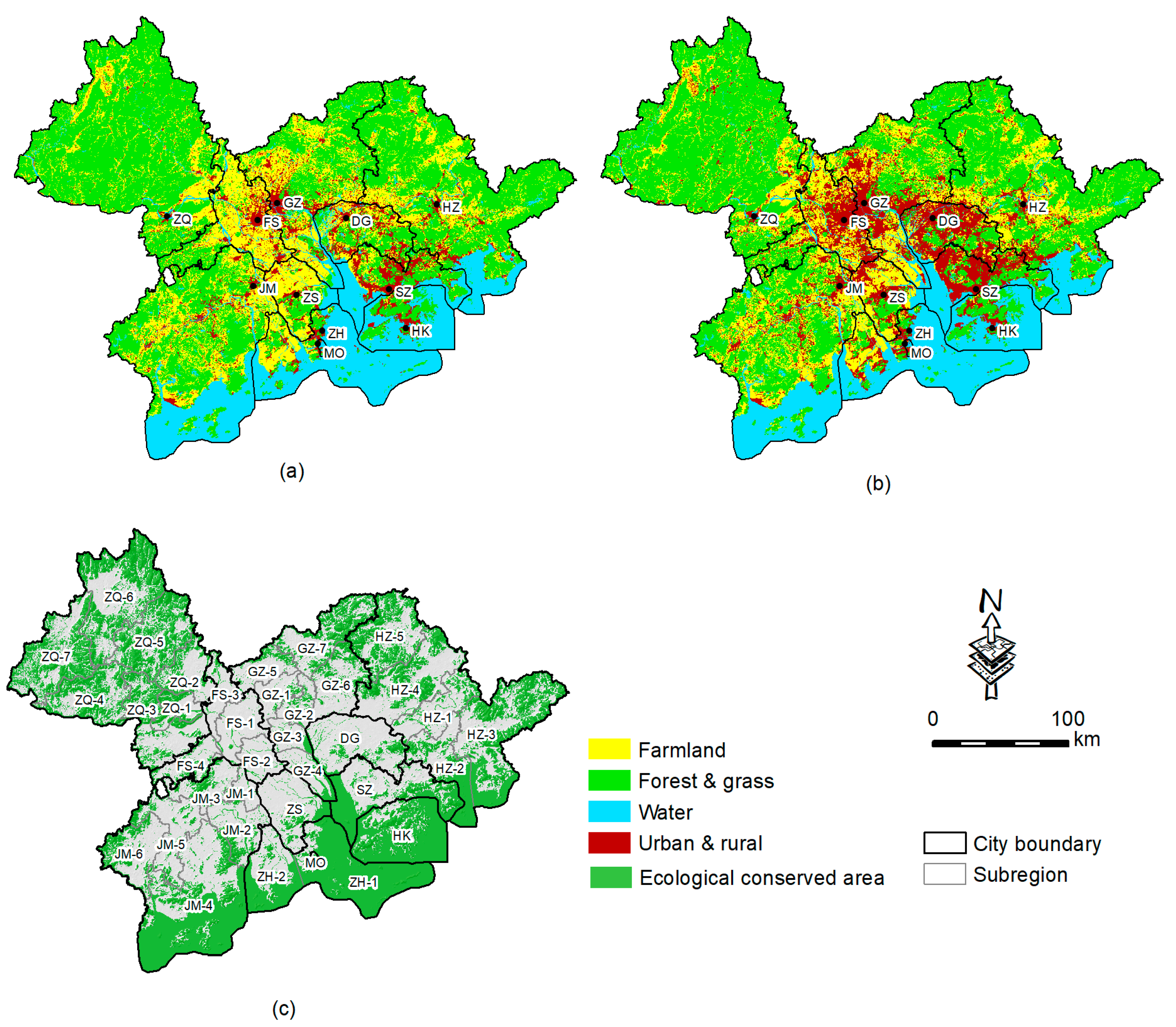
2.2.1. Land Use Cover/Change, Subzones, and Ecological Sensitive Areas

To use the spatial Markov chain model for quantitative urban land-use predictions, it was necessary to ascertain the transfer probability at equivalent time steps. For this purpose, historical Landsat satellite images of the GBA in 1995 and 2015 were collected, and land use was obtained using the human–computer interaction interpretation method for both years (Figure 2a,b). From the land-use change between 1995 and 2015, it was clear that the urban area had grown rapidly over the previous 20 years, and there was little available land left in eastern Bay Area cities such as Shenzhen and Dongguan. Given these characteristics, we understood that using the Markov process to predict change over the next 20 years would lead to obvious inaccuracies caused by the incompatibility of spatial units. In response, this study took as a reference the “nomenclature of territorial units for statistics” classification used for spatial planning within the European Union (EU) [63]. It allowed us to merge county-level units in the central areas of large cities without destroying the urban boundary and having to construct a new unit for the spatial Markov analysis. For example, Guangzhou originally had 11 county-level units—Yuexiu, Liwan, Haizhu, Tianhe, Baiyun, Huangpu, Panyu, Huadu, Nansha, Zengcheng, and Conghua—but these were reduced to 7 after the spatial reorganization of Yuexiu, Liwan, and Baiyun into a new subzone, “GZ-1.” The GBA’s 49 county-level units and 2 special administrative regions became 36 standard subzones after the spatial merger (Figure 2c). To simulate the future growth of an urban agglomeration, it was necessary to not only monitor historical development to discover trends but also establish ecological constraints. The geography of the GBA is characterized by relative height differences of more than 60 m due to mountains, a large river, a reservoir, coastal areas, and high-density forest land. If the maximum urban growth were not to exceed the upper limit of ecologically sensitive areas, all these areas had to be excluded (Figure 2c).

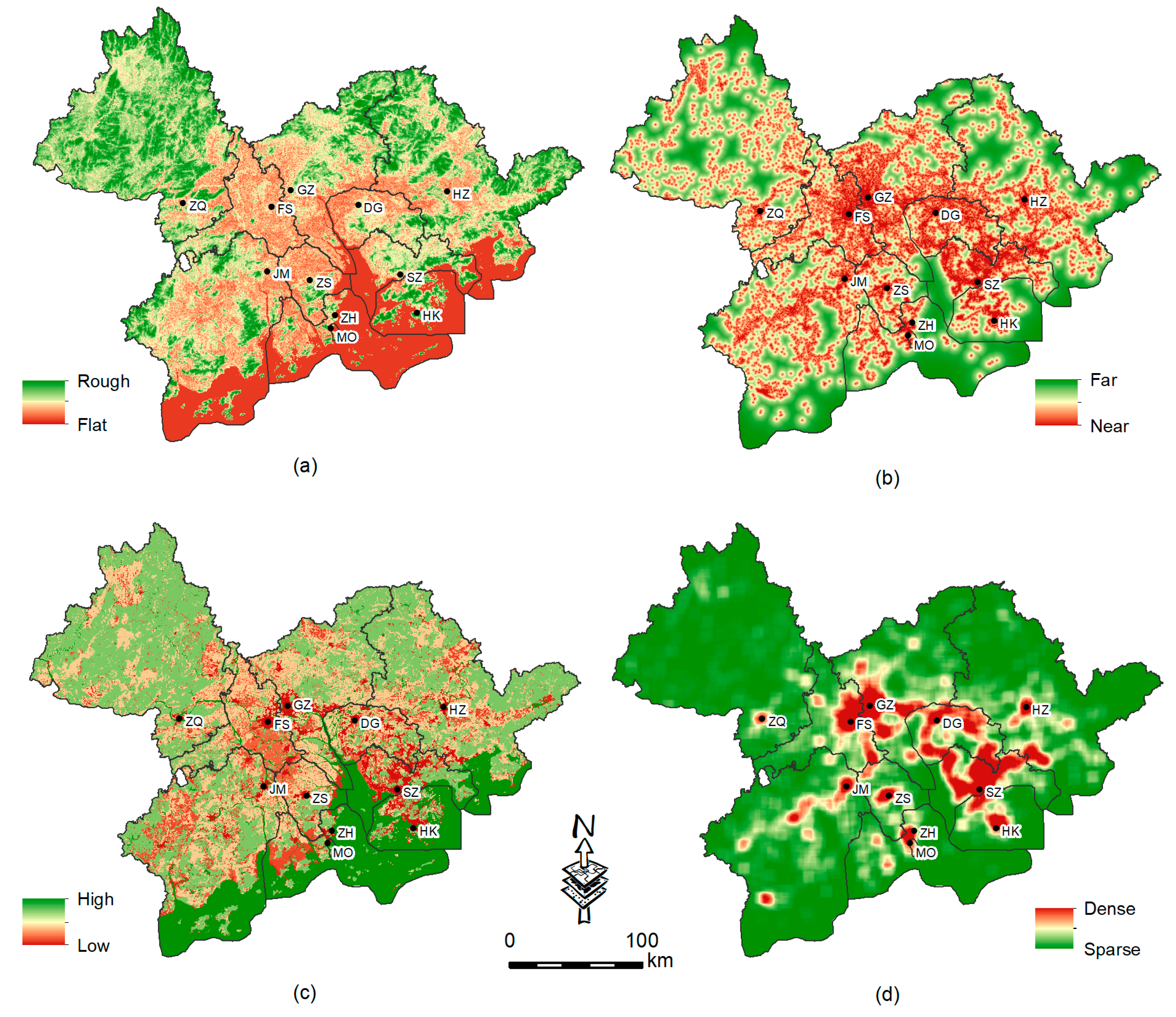
2.2.2. Spatial Variables for Evaluating Suitable Urban Growth

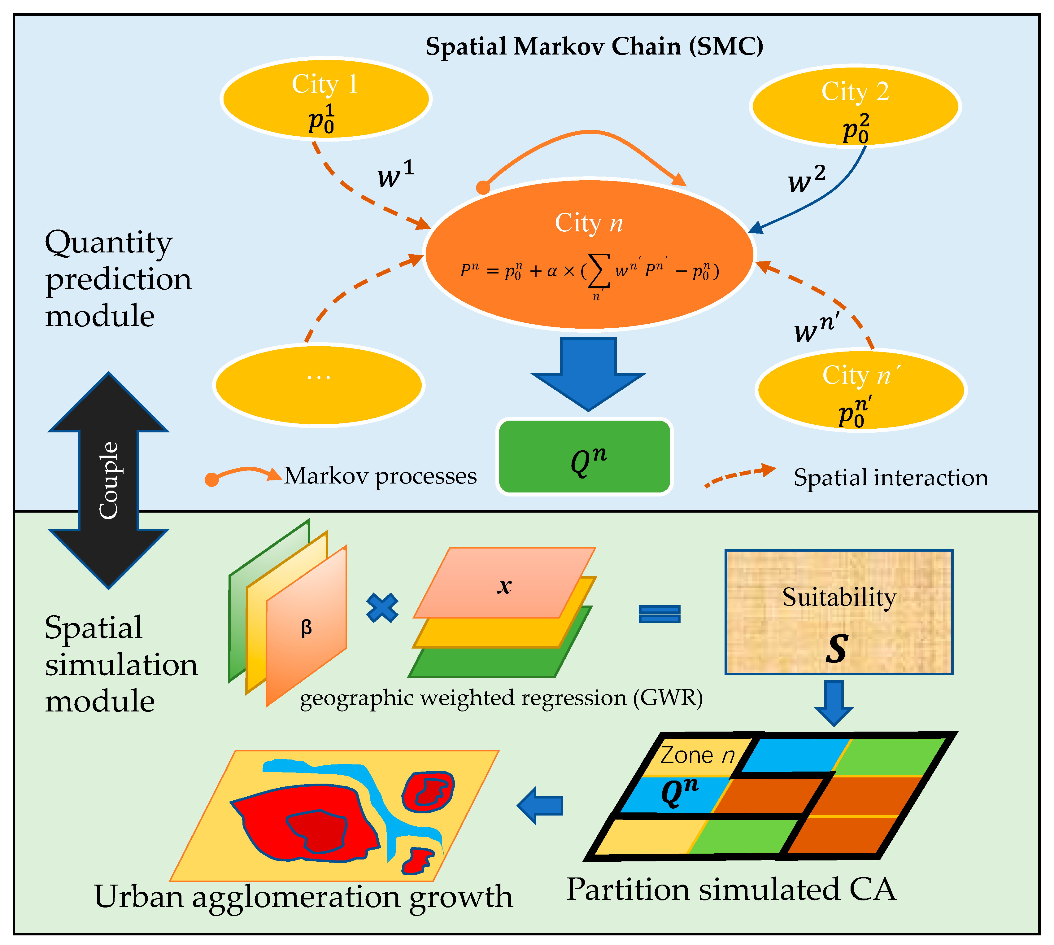
In addition to analyzing historical land-use change using the SMC approach, this study also evaluated urban growth suitability using the GWR model. Generally, many spatial factors need to be considered in evaluating urban growth suitability [35,52]. However, given that the present study performed such an evaluation on the scale of an urban agglomeration—especially since we used the Markov chain to reconstruct the spatial structure of the GBA—we felt that it was better to choose relatively few but highly stable spatial factors. As such, only four variables were used to investigate urban agglomeration growth: terrain flatness, distance to existing cities and towns, land-use conversion cost, and urban landscape density. “Terrain flatness”, which reflects the spatial conditions for construction, can be calculated as the relative height difference through a digital elevation model (DEM) with a dynamic, 1 km² window (Figure 3a). “Distance from existing built-up land” was measured in 1995 mainly using Euclidean distance (Figure 3b). The “cost of land-use conversion” reflects the cost of converting different types of land into “built-up land”, and for this measure, we were able to refer to the government’s formulation of compensation standards for land acquisition (Figure 3c). “Urban landscape density” reflects the spatial pattern of an agglomeration on a large (regional) scale and can be estimated using a large, 10 km² window (Figure 3d). In addition to these four independent variables, urban growth between 1995 and 2015 constituted a dependent variable, and urban growth was a logical variable, which needed to be changed into a probability value before being used in a geographically weighted regression analysis. In this study, we used the Moore neighborhood resampling technique to change the discrete value of 0.1 to a continuous value range from 0 to 1.

2.3. Methodology

The growth of urban agglomeration includes two main aspects: the urban built-up land scale growth for each city, and the spatial form evolution under the corresponding space scale. In this paper, the SMC and GWRCA were used to simulate urban agglomeration growth, and the model flow chart is shown in Figure 4. The coupling model includes two submodules: quantity prediction and spatial form evolution. Quantity prediction is based on the classical Markov model, but interaction with an urban agglomeration should be considered a transition probability. The spatial form evolution module used a GWR model to estimate the initial growth probability and then used neighborhood interactions of CA to simulate the change in spatial morphology. The relevant model principles are discussed in Section 2.3.1 and Section 2.3.2.

2.3.1. Spatial Markov Chain

The Markov chain (MC) is a stochastic process that is often used to predict changes in land-use structure [21,35,64] and a Markov model can be expressed by Equation (1):

$$Q^n(t)=Q^n(t-1)\times P^n\hspace{1em}\hspace{1em}\hspace{1em}\hspace{1em}{P}^n\le P_{\max }^n$$

(1)

where $Q^n(t)$ and $Q^n(t-1)$ represents the quantity of at time t and t − 1, and Pⁿ is the transition probability matrix. In general, Pⁿ can be extracted from the historical urban growth process of subzone n, but it is necessary to ensure that there is no obvious mutation in the rate of change. Because China expects to conclude rapid urbanization by 2050, we assumed that the simulation of change from 2015 to 2050 could build on the transfer probability obtained from changes from 1995 to 2015. We acknowledged that change is also affected by government policies (for instance, ecological protection measures) and that the transfer matrix Pⁿ cannot be increased indefinitely—it must remain within the maximum increase range of the region. In other words, $Q^n\le Q_{\max }^n$. $Q_{\max }^n$ is the maximum amount that can be used for urban growth, excluding ecological or farmland protection.

Traditional Markov processes tend to construct one comprehensive land-use transfer matrix, which is effective for a single city but not suitable for an urban agglomeration. Since each city in an agglomeration maintains a relatively independent development authority, a Markov process must be established for each one. However, if the whole agglomeration were simply divided into multiple independent Markov processes, it would not be possible to describe the essential character of the urban agglomeration as a system because each city engages with, and exerts influence over, other cities. To fully consider the space-time interactions among the cities in the GBA, we proposed using a spatial Markov chain. The SMC considered not only the transfer probability of each unit but also the driving effects exerted by surrounding cities. As such, if a spatial Markov analysis showed the growth rate of comprehensive radiation around a city to be higher than the speed of the city’s growth, then the city is said to exhibit an accelerating growth trend; on the other hand, if the growth rate of the surrounding cities is lower, then the city may be the growth pole. Therefore, a city may change its own growth speed and potential speed in line with the effects of surrounding cities. The modified $P$ can be calculated by Equation (2):

$$P^n=P_0^{\mathrm{n}}+\alpha \times \left({\displaystyle {\sum }_{n\prime }{w}^{n\prime }{p}^{n\prime }-P^n}\right), n\prime \ne n$$

(2)

where ${\sum }_{n\prime }{w}^{n\prime }{p}^{n\prime }$ represents the comprehensive interaction effect from the surrounding cities n’ (n’ ≠ n); the coefficient $w^{n\prime }$ can be set by the method of inverse distance. ${\displaystyle {\sum }_{n\prime }{w}^{n\prime }{p}^{n\prime }-P^n}$ is the difference between the transfer value from the surrounding cities and its own value. If this value is positive, it indicates that the surrounding cities exert a pulling effect; if it is negative, they exert a slowing effect or no effect. α is the adjustment coefficient which ranges from 0 to 1, it is used to describe the radiation-driven intensity of the effect of the surrounding subregions (or cities) on subregion n. If α = 1, it means that subregion n is completely affected by its surrounding subregions; conversely, if α = 0, it indicates that subregion n is completely unaffected. Otherwise, it is affected by a degree of interaction effect from surrounding subregions.

2.3.2. Geographically Weighted Regression Based on Cellular Automata

Because the SMC model can only predict the quantity of built-up land in each subregion [60], we also employed a spatial evolution model to simulate the corresponding spatial pattern. Cellular automata (CA), which are able to achieve dynamic results by means of simple rules, have become important in urban growth simulations [65]. A typical CA simulation framework can be expressed as in Equation (3):

$$U_{ij}^n\left(t\right)=f\left(Q^n\left(t\right),S_{ij},{\Omega }_{ij}\left(t\right),{\Psi }_{ij}\right)$$

(3)

where $U_{ij}^n\left(t\right)$ represents the state of cell ij at time t in subzone n, (e.g., 0 means non-growth and 1 means growth); function f is the iterative operation of CA, which produces a series of spatial factors, including the suitability of urban growth, and neighborhood interaction; $Q^n\left(t\right)$ represents the quantity of the demand for urban land in subzone n at time t; S_ij is the suitability of cell ij for urban growth, which is usually estimated by means of data mining techniques such as regression analysis; ${\Omega }_{ij}\left(t\right)$ indicates that cell ij is affected by the development of neighboring cells at time t, which can be characterized as development density; ${\Psi }_{ij}$ denotes policy restrictions that prevent development (e.g., ecological conservation measures).

In a CA model, both $Q^n\left(t\right)$ and ${\Psi }_{ij}$ are external input parameters, and ${\Omega }_{ij}\left(t\right)$ is only related to the window size calculation. As such, the most important parameter affecting the spatial pattern is suitability, and the simulation scenarios that CA works with rely mainly on the generation of a suitability map. In previous studies, it was commonly estimated by means of sample data mining, which was also used in this paper. In this study, pronounced geographical spatial differentiation was present due to the size of the urban agglomeration we addressed. If the overall parameter estimation were used in such a situation, the individual differences of the study area (the GBA urban agglomeration) could easily be missed; conversely, if each city were analyzed separately, it would split the overall relationship of the groups. Given these limitations, we also employed the classical method of geographically weighted regression (GWR) to calculate the suitability map [61]. The GWR, essentially an extension of the ordinary linear regression (OLR) model, is predominantly used to analyze spatial heterogeneity by considering local autocorrelation. If the local space is extended to the global, then the GWR will be transformed into an OLR. A standard GWR model is as follows:

$$y_{ij}={\beta }_{ij0}+{\displaystyle {\sum }_{k=1}^k{\beta }_{ijk}{x}_{ijk}}+{\epsilon }_{ij}$$

(4)

where y_ij is a dependent variable describing the probability of land constituting built-up land; ij is the position coordinate of cell ij, which can be expressed as longitude and latitude or as a row-and-column index in raster data format; and ${\beta }_{ijk}$ is the k-th regression coefficient. We noted that, as opposed to the OLR, each spatial factor in the GWR had different coefficients. In the above formula, ${\epsilon }_{ij}$ is the model estimation error term, which satisfied the normal distribution. Using a coefficient matrix and the spatial factors obtained through the GWR, the suitability values of all positions were estimated. In practice, the suitability evaluation cannot be based completely on the results of data mining; it can be fine-tuned in accordance with the strategic aims for spatial development contained in relevant plans for the area.

3. Results

3.1. Quantity Prediction With the SMC

Table 1. Quantity of built-up land in 2050 within the GBA (km²).

Index	Cities	Total Quantity	Subregion	Quantity
1	GZ	3152.88	GZ-1	589.23
			GZ-2	488.7
			GZ-3	500.85
			GZ-4	399.96
			GZ-5	413.37
			GZ-6	565.2
			GZ-7	195.57
2	SZ	1434.96	/	/
3	ZH	712.17	ZH-1	278.28
			ZH-2	433.89
4	FS	2057.22	FS-1	910.08
			FS-2	593.82
			FS-3	303.12
			FS-4	250.2
5	HZ	1419.39	HZ-1	356.94
			HZ-2	386.19
			HZ-3	244.53
			HZ-4	302.85
			HZ-5	128.88
6	DG	1864.71	/	/
7	ZS	844.29	/	/
8	JM	1660.68	JM-1	297.63
			JM-2	312.12
			JM-3	240.3
			JM-4	366.39
			JM-5	233.37
			JM-6	210.87
9	ZQ	1084.41	ZQ-1	226.35
			ZQ-2	256.68
			ZQ-3	187.38
			ZQ-4	82.35
			ZQ-5	98.1
			ZQ-6	145.08
			ZQ-7	88.47
10	HK	442.8	/	/
11	MO	26.1	/	/
12	GBA	14,699.61	/	/

shows the results of our size estimate of the GBA urban area and its subregions in 2050. According to the results from the SMC model, the total area will grow to 14,699.61 km², and within that urban agglomeration, Guangzhou will be the largest city because the amount of land available for development is relatively large and the strength of the city’s social and economic development will stimulate adequate demand. However, quantity analysis alone cannot provide an image of how the GBA will develop. In addition, from a historical development perspective, our results showed that the GBA will enter the mature development stage by 2050.

3.2. Growth Scenario of the SMC-GWRCA Model

Spatial pattern simulation is helpful for scholars to understand development trends in urban agglomerations, and it provides support for decisions regarding infrastructure construction. The growth scenario for China’s GBA simulated in this study using the SMC-GWRCA model is shown in Figure 5a. To analyze the reliability of the results further, the simulation pattern for 2050 was transformed into a series of urban growth boundaries (UGBs), which are shown as red lines in Figure 5. Furthermore, the highest resolution image provided by Google Earth in 2019 was used to further review the rationality of the simulation results (Figure 5b,c). From Figure 5, some inconsistencies between the UGB and the actual geographical features can be seen, but these can be attributed to restrictions in data refinement. We acknowledge that, in any practical application, our findings for the simulation results would need to be modified manually to meet these control boundary conditions. However, for the purposes of the quantitative modeling discussed in this paper, we chose to focus our analysis on the overall pattern and not address areas where boundary details were inconsistent. We selected two typical areas from the GBA for discussion, and these are marked as the rectangular zones A and B. Zone A is located in the northeastern part of Zhaoqing, a city on the edge of the GBA. Judging from the remote sensing image, the urban growth that occurred in this area between 2015 and 2019 was almost totally within the UGB. Further analysis revealed the formation of a street network in region A1, and a great deal of built-up land emerged in region B1. In general, our simulation results for the GBA using the SMC-GWRCA model are considered feasible.

4. Discussion

4.1. Spatiotemporal Interaction of Urban Agglomeration

To evaluate whether the SMC method is more suitable than the MC method for predicting the development of urban agglomerations, we analyzed historical changes in the whole GBA urban agglomeration and compared them with the results of a traditional MC prediction.

Table 2. Historical change and model predictions for the GBA (km²).

Subregion	Quantity in 1995	Quantity in 2015	Maximum for Growth	Quantity in 2050
				Predicted with MC	Predicted with SMC	Difference between MC and SMC
GZ-1	216.63	355.32	655.83	494.01	589.23	95.22
GZ-2	156.78	271.26	488.7	385.74	488.70	102.96
GZ-3	161.73	317.61	500.85	473.49	500.85	27.36
GZ-4	55.35	144.81	542.34	234.27	399.96	165.69
GZ-5	82.17	238.77	738	395.37	413.37	18
GZ-6	118.71	236.7	1124.55	354.69	565.20	210.51
GZ-7	53.01	104.04	997.29	155.07	195.57	40.5
SZ	652.32	1084.23	1434.96	1434.96	1434.96	0
ZH-1	107.1	180.9	278.28	254.7	278.28	23.58
ZH-2	105.75	258.84	862.47	411.93	433.89	21.96
FS-1	316.35	666.09	1144.17	1015.83	910.08	−05.75
FS-2	148.95	375.03	751.59	601.11	593.82	−7.29
FS-3	42.21	145.98	698.67	249.75	303.12	53.37
FS-4	49.41	118.71	682.2	188.01	250.20	62.19
HZ-1	149.13	255.78	1104.03	362.43	356.94	−5.49
HZ-2	175.05	285.75	802.35	396.45	386.19	−10.26
HZ-3	110.79	163.71	1641.87	216.63	244.53	27.9
HZ-4	90.27	198.81	1740.96	307.35	302.85	−4.5
HZ-5	25.47	58.23	958.95	90.99	128.88	37.89
DG	593.64	1363.05	2031.93	2031.93	1864.71	−167.22
ZS	200.7	554.4	1473.66	908.1	844.29	−63.81
JM-1	72.09	155.52	369.54	238.95	297.63	58.68
JM-2	107.55	185.4	983.34	263.25	312.12	48.87
JM-3	47.43	110.79	773.82	174.15	240.30	66.15
JM-4	158.22	269.46	2067.66	380.7	366.39	−14.31
JM-5	98.64	157.77	1284.48	216.9	233.37	16.47
JM-6	73.35	134.91	1070.19	196.47	210.87	14.4
ZQ-1	41.85	68.49	339.39	95.13	226.35	131.22
ZQ-2	40.59	120.87	814.23	201.15	256.68	55.53
ZQ-3	55.71	122.85	1254.87	189.99	187.38	−2.61
ZQ-4	17.01	50.13	862.74	83.25	82.35	−0.9
ZQ-5	23.04	52.56	866.88	82.08	98.10	16.02
ZQ-6	45.09	101.88	1577.43	158.67	145.08	−13.59
ZQ-7	24.93	56.25	1176.48	87.57	88.47	0.9
HK	252.09	293.67	442.8	335.25	442.80	107.55
MO	14.04	24.12	26.1	26.1	26.10	0
GBA	4683.15	9282.69	34,563.6	13,692.42	14,699.61	1007.19

shows the quantity of built-up land in the GBA with respect to historical changes and our forecast. In 1995, an area of about 4683.15 km² was dedicated for urban development, but by 2015 this area had grown to 9282.69 km², an increase of 4599.54 km² over 20 years. Excluding ecological reserves, the maximum area available for urbanization was 34,563.60 km², which shows that the GBA retained a significant degree of overall development potential. However, the process of urbanization differed among subregions. For example, the current scale of development in Dongguan (DG), Shenzhen (SZ), Hong Kong (HK), and Macao (MO) is very high but constrained by ecological conservation areas, which severely restrict expansion. In these cases, potential development demands can be transmitted to surrounding cities through radiation effects.

The prediction results of the SMC for each subregion showed that the growth rates of some subregions will increase, while others will be expected to slow. For example, in the DG subregion, the MC prediction result was 2031.93 km², which indicated that the subregion will reach its maximum growth limit in the next 20 years, but the SMC prediction suggested only 1864.71 km², a reduction of 167.22 km² that can be expected to be transmitted to surrounding cities. Among these subregions, MO is fully urbanized, and without land reclamation, there is no space for growth. In addition, the density of urban development in HK is already very high, and there is a great demand for growth. However, the government’s compulsory control makes reserve land resources in HK temporarily unavailable for development. This paper did not consider the problems caused by this complex administrative system. Development intensity in the GBA (total built-up land/total land area) was found to be 7% in 1995 and 14% in 2015, and the results of the SMC modeling projected a rise to about 26% for 2050. Although the overall development intensity was shown to be relatively low, it was different for each city. For example, the development intensity of GZ-1, GZ-2, GZ-3, SZ, FS-1, FS-2, DG, and other regions all exceeded 50%, and some of these subregions were identified as approaching the upper limit of development. Compared with the MC prediction, the results obtained from the SMC increased by 1007.19 km², with an average of fewer than 30 km² for 36 units, which can be read as denoting uncertainty or elastic space. Compared with the MC prediction, the results of the SMC show future development trends within the GBA more accurately.

4.2. Geographical Spatial Differentiation in Urban Agglomerations

Urban development is very sensitive to spatial conditions like terrain and other spatial factors, and for this reason, it is difficult to simulate real urban spatiotemporal evolution if the urban CA is not corrected by the geospatial environment. In performing a regression analysis, this study took urban spatial change between 1995 and 2015 as the dependent variable, which we analyzed in relation to four spatial variables: terrain conditions, distance to existing urban areas, land-use conversion cost, and urban landscape pattern. In this study, 59,777 training samples were randomly sampled from one sample point per square kilometer. We then used statistical analysis tools provided by ArcGIS to model suitability evolution. Regression results first needed to be adjusted manually before simulation through a procedure where we set to 0 the ecologically sensitive areas where development is prohibited and then enhanced the spatial development probability along the coast of the GBA (the elliptical region in Figure 6) by increasing it by 0.05 for each cell. Due to the large area of the urban agglomeration, there was obvious geographical spatial differentiation. If traditional overall estimation, rather than a local estimation, is used with such preconditions, it may not be able to give an accurate analysis. The spatial driving probability results of the GWR and OLR models are shown in Figure 6. Compared with the OLR’s global average estimation, the GWR balanced the development differences in relation to urban agglomerations better. The results of the OLR model indicated that peripheral cities such as Jiangmen, Huizhou, Zhaoqing, are basically devoid of high development probability results. If this kind of spatial probability is used to drive the development of an urban agglomeration, these cities will have reduced development opportunities, which is obviously not in line with the trend toward integrated development within the GBA. Therefore, we believe that it is necessary to consider spatial autocorrelation in urban agglomeration simulation. Moreover, the suitability of data estimation based on historical change can only represent the law of historical processes, which does not mean that future urbanization will be the same. Given this, it is necessary to revise the suitability map manually for regions with obvious spatial development policy regulation; otherwise, the CA model will have difficulty simulating the expected pattern.

4.3. Advantages of the SMC-GWRCA for Urban Agglomeration Simulation

To analyze the advantages of the SMC-GWRCA for simulating the GBA spatial pattern in 2050, all parameters of the CA model employed in this paper were set conventionally (e.g., Ω adopted the conventional Moore neighborhood, and neighborhood Ω and suitability S were coupled with equal weight). The total number of iterations of the GWRCA was 200 (10 iterations per year), and each iteration was an equivalent conversion. The simulation patterns for the GBA in 2050 obtained by coupling the SMC-GWRCA, MC-GWRCA, SMC-OLRCA, and MC-OLRCA models are shown in Figure 7. From these results, the spatial patterns simulated by the four models were quite different though they worked under largely the same parameters (except Q and S). To analyze whether the MC or SMC prediction results were more reasonable, the subregion marked as GZ-4 in Figure 7 was used as an example for comparative analysis. GZ-4 is the Nansha New Area, which has been planned as the Vice-Center of Guangzhou, and is bound to be subjected to strong growth trends. Using only the MC method, projected increases up to 2050 are expected to be small due to the low level of historical transformation between 1995 and 2015. On the other hand, the SMC was able to take into account the radiation of high-speed growth cities in the east such as SZ and DG. In the past, the eastern part of the GBA was largely disconnected from the western, but this is no longer the case as the east–west connection across is becoming increasingly convenient: the Hong Kong–Zhuhai–Macao, Humen, and Nansha bridges have all been opened, and the Shenzhen–Zhongshan channel is under construction. From this evidence, we can see that the SMC constitutes a more reasonable method than the MC. Comparing the GWR and OLR methods, the patterns derived through OLR simulation are concentrated around big cities, while the peripheral areas were too scattered, which conclusively demonstrates that the GWR is the more suitable for urban agglomeration simulation.

From the view of spatial patterns, the development scenario simulation with the SMC-GWRCA model was more consistent with actual requirements. To further evaluate the differences among the four simulation models, the urban agglomeration pattern observed by remote sensing in 2020 was compared with that simulated by each model in this study, and the accuracy was evaluated by the Figure of Merit (FOM) index, which was significantly higher because the detection time was short) [66,67] (

Table 3. Simulation precision testing of four models.

	SMC-GWRCA	SMC-OLRCA	MC-GWRCA	MC-OLRCA
FOM	0.6881	0.6336	0.6021	0.5830
PA	81.53%	79.10%	75.16%	72.77%

). We found that the accuracy of the SMC-GWRCA model was better than the others for the FOM shape index and prediction accuracy (PA). For example, the FOM index of the SMC-GWRCA was 0.6881, higher than that of classical MC-OLRCA, and the prediction accuracy improved from 72.77 to 81.53%. This indicated that more than 80% of the new units predicted by the SMC-GWRCA from 2015 to 2020 had occurred, and the improved model can better simulate the development of new areas. Overall, the SMC-GWR coupling model was a great improvement over the traditional model (the SMC for quantity prediction and the GWR for spatial form evolution) and showed that the urban agglomeration scale must take into account the interaction between cities and spatial differentiation. Urban agglomeration simulation cannot simply copy the classical CA modeling process.

5. Conclusions

As urbanization reaches an advanced stage globally, agglomerations have emerged as an increasingly prevalent form of spatial organization. Their development trends must be analyzed to provide a more scientific basis for spatial planning decisions, such as how to optimize infrastructure networks for optimal group connection. However, as the research object shifts from single cities to groups of cities, the scale of the geographical space being studied can become very large, and interactions among cities become more and more obvious, so it is very important to establish an effective simulation method to deal with these. To simulate the spatiotemporal evolution of urban agglomerations, this study introduced a simulation model that integrated the spatial Markov chain and the geographic-weighted regression-based cellular automata methods. The effect of the model was analyzed in relation to the Guangdong–Hong Kong–Macao Greater Bay Area (GBA) urban agglomeration.

This research shows that the spatial Markov chain was fully able to reflect radiation-driven utility among the cities, and taking these intercity interactions into account, the development of the urban agglomeration was reconstructed and projected. Taking the Nansha New Area, the geometric center of the GBA as an example, we noted that little obvious urban growth occurred in the period 1995–2015. However, this area is expected to become the Vice-Center of Guangzhou and is bound to face large-scale growth demands. This kind of demand cannot be predicted by means of a traditional MC process. The SMC approach, however, can deal with the radiation of the development demand of surrounding areas. The Nansha New Area, as the geometric center of GBA, is bound to receive the most intense radiation from surrounding cities. Our comparison of the simulation results obtained under these two methods fully supports this conclusion.

There is no doubt that using a spatial Markov chain model to simulate the quantity structure of urban agglomerations is feasible, but the spatial Markov model also has application limitations. First, it must assume that the transfer process is relatively stable, which is deeply related to the urbanization stage of the agglomeration or its region. If the region has reached the mature stage, even if there has been a past large-scale transformation, this principle cannot be used to predict the next stage of transformation. To eliminate this potential limitation, we drew inspiration from the European Union’s nomenclature of territorial units for statistics and merged a number of urban core areas to ensure the trend of analysis unit transfer. Second, the spatial Markov chain still needs to verify the strength of the interactions among the cities in an urban agglomeration. In this paper, inverse-distance weighting was used directly, but we noted that the method for defining the interaction between cities scientifically requires further exploration.

In the spatial pattern simulation performed in this paper, four driving factors were selected for their stability to mine the urban growth probability. Factors such as the street network and the location of development centers, which are used in traditional CA simulation, were not used. Because their quantities vary over time, such factors cannot be used to explain the drivers of the long-term development of urban agglomerations. For example, a new highway or subway built by the government can completely change this pattern of drivers. For this reason, we maintain that it is more appropriate to use spatially stable factors to explain the long-term spatial patterns of the drivers of urban development when research is conducted on the scale of the urban agglomeration.

In addition, the question of how to integrate quantitative data mining methods to identify drivers and qualitative spatial policy regulation to form a more accurate fitness map are both key points for simulating the long-term growth of urban agglomerations. Our research showed that it is feasible to extract the driving force coefficients of various spatial factors from historical urban growth. Compared with the global regression method, we considered the geographic-weighted regression method to be more suitable for analyzing the urban agglomeration. However, studying historical change can only provide insight into the past development of urban agglomerations, trends that will not necessarily continue. A new development strategy from government spatial planners can completely change the previous development model. As such, research must combine qualitative and quantitative methods in simulations, and avoid overreliance on purely quantitative results. The model is, after all, only a model.

Although there are many limitations to spatial planning scenario analyses, we believe that as long as the simulation model is fed enough refined data, the SMC-GWRCA method can competently simulate the spatiotemporal evolution process of urban agglomerations. In general, simulation models can help us understand the development mechanisms at work and provide a reference for decision-making within territorial spatial planning. The simulation framework studied in this paper only needed a small amount of data and a limited number of parameters to simulate the growth of urban agglomerations. Through future research, we would like to try a larger-scale simulation, such as modeling urban agglomerations over the whole of China.

References

1. Liu, X.; Hu, G.; Chen, Y.; Li, X.; Xu, X.; Li, S.; Pei, F.; Wang, S. High-resolution multi-temporal mapping of global urban land using Landsat images based on the Google Earth Engine Platform. Remote Sens. Environ. 2018, 209, 227–239. [Google Scholar] [CrossRef]
2. Zhou, Y.; Li, X.; Asrar, G.R.; Smith, S.J.; Imhoff, M. A global record of annual urban dynamics (1992–2013) from nighttime lights. Remote Sens. Environ. 2018, 219, 206–220. [Google Scholar] [CrossRef]
3. Xu, Y.; Yu, L.; Peng, D.; Zhao, J.; Cheng, Y.; Liu, X.; Li, W.; Meng, R.; Xu, X.; Gong, P. Annual 30-m land use/land cover maps of China for 1980–2015 from the integration of AVHRR, MODIS and Landsat data using the BFAST algorithm. Sci. China Ser. D Earth Sci. 2020, 63, 1390–1407. [Google Scholar] [CrossRef]
4. McDonald, R.I. Global urbanization: Can ecologists identify a sustainable way forward? Front. Ecol. Environ. 2008, 6, 99–104. [Google Scholar] [CrossRef]
5. Seto, K.C.; Sanchezrodriguez, R.; Fragkias, M. The new geography of contemporary urbanization and the environment. Annu. Rev. Environ. Resour. 2010, 35, 167–194. [Google Scholar] [CrossRef] [Green Version]
6. Seto, K.C.; Güneralp, B.; Hutyra, L.R. Global forecasts of urban expansion to 2030 and direct impacts on biodiversity and carbon pools. Proc. Nat. Acad. Sci. USA 2012, 109, 16083–16088. [Google Scholar] [CrossRef] [PubMed] [Green Version]
7. Shen, L.; Shuai, C.; Jiao, L.; Tan, Y.; Song, X. A global perspective on the sustainable performance of urbanization. Sustainability 2016, 8, 783. [Google Scholar] [CrossRef] [Green Version]
8. Mulligan, G.F. Revisiting the urbanization curve. Cities 2013, 32, 113–122. [Google Scholar] [CrossRef]
9. National Bureau of Statistics, China. Available online: http://www.stats.gov.cn/english/ (accessed on 9 December 2020).
10. Cao, S.; Lv, Y.; Zheng, H.; Wang, X. Challenges facing China’s unbalanced urbanization strategy. Land Use Policy 2014, 39, 412–415. [Google Scholar] [CrossRef]
11. Cheshmehzangi, A. China’s New-type Urbanisation Plan (NUP) and the foreseeing challenges for decarbonization of cities: A review. Energy Procedia 2016, 104, 146–152. [Google Scholar] [CrossRef]
12. Guan, X.; Wei, H.; Lu, S.; Dai, Q.; Su, H. Assessment on the urbanization strategy in China: Achievements, challenges and reflections. Habitat Int. 2018, 71, 97–109. [Google Scholar] [CrossRef]
13. Rounsevell, M.D.A.; Pedroli, B.; Erb, K.; Gramberger, M.; Busck, A.G.; Haberl, H.; Kristensen, S.; Kuemmerle, T.; Lavorel, S.; Lindner, M.; et al. Challenges for land system science. Land Use Policy 2012, 29, 899–910. [Google Scholar] [CrossRef]
14. Santé, I.; García, A.M.; Miranda, D.; Crecente, R. Cellular automata models for the simulation of real-world urban processes: A review and analysis. Landsc. Urban. Plan. 2010, 96, 108–122. [Google Scholar] [CrossRef]
15. Aburas, M.M.; Ho, Y.M.; Ramli, M.F.; Ash Aari, Z.H. The simulation and prediction of spatio-temporal urban growth trends using cellular automata models: A review. Int. J. Appl. Earth Obs. 2016, 52, 380–389. [Google Scholar] [CrossRef]
16. Le, Q.B.; Park, S.J.; Vlek, P.L.G.; Cremers, A.B. Land-Use Dynamic Simulator (LUDAS): A multi-agent system model for simulating spatio-temporal dynamics of coupled human–landscape system. I. Structure and theoretical specification. Ecol. Inform. 2008, 3, 135–153. [Google Scholar] [CrossRef]
17. Le, Q.B.; Park, S.J.; Vlek, P.L.G. Land Use Dynamic Simulator (LUDAS): A multi-agent system model for simulating spatio-temporal dynamics of coupled human–landscape system: 2. Scenario-based application for impact assessment of land-use policies. Ecol. Inform. 2010, 5, 203–221. [Google Scholar] [CrossRef]
18. Li, X.; Gong, P. Urban growth models: Progress and perspective. Sci. Bull. 2016, 61, 1637–1650. [Google Scholar] [CrossRef]
19. Okwuashi, O.; Ndehedehe, C.E. Integrating machine learning with Markov chain and cellular automata models for modelling urban land use change. Remote Sens. Appl. Soc. Environ. 2021, 21, 100461. [Google Scholar]
20. Xu, X.; Du, Z.; Zhang, H. Integrating the system dynamic and cellular automata models to predict land use and land cover change. Int. J. Appl. Earth Obs. 2016, 52, 568–579. [Google Scholar] [CrossRef]
21. Jokar Arsanjani, J.; Helbich, M.; Kainz, W.; Darvishi Boloorani, A. Integration of logistic regression, Markov chain and cellular automata models to simulate urban expansion. Int. J. Appl. Earth Obs. 2013, 21, 265–275. [Google Scholar] [CrossRef]
22. Cunha, E.R.D.; Santos, C.A.G.; Silva, R.M.D.; Bacani, V.M.; Pott, A. Future scenarios based on a CA-Markov land use and land cover simulation model for a tropical humid basin in the Cerrado/Atlantic forest ecotone of Brazil. Land Use Policy 2021, 101, 105141. [Google Scholar] [CrossRef]
23. Rahnama, M.R. Forecasting land-use changes in Mashhad Metropolitan area using Cellular Automata and Markov chain model for 2016–2030. Sustain. Cities Soc. 2021, 64, 102548. [Google Scholar] [CrossRef]
24. Mansour, S.; Al-Belushi, M.; Al-Awadhi, T. Monitoring land use and land cover changes in the mountainous cities of Oman using GIS and CA-Markov modelling techniques. Land Use Policy 2020, 91, 104414. [Google Scholar] [CrossRef]
25. Palmate, S.S.; Pandey, A.; Mishra, S.K. Modelling spatiotemporal land dynamics for a trans-boundary river basin using integrated Cellular Automata and Markov Chain approach. Appl. Geogr. 2017, 82, 11–23. [Google Scholar] [CrossRef]
26. Yang, X.; Zheng, X.; Lv, L. A spatiotemporal model of land use change based on ant colony optimization, Markov chain and cellular automata. Ecol. Model. 2012, 233, 11–19. [Google Scholar] [CrossRef]
27. Rasmussen, L.V.; Rasmussen, K.; Reenberg, A.; Proud, S. A system dynamics approach to land use changes in agro-pastoral systems on the desert margins of Sahel. Agric. Syst. 2012, 107, 56–64. [Google Scholar] [CrossRef]
28. Liu, X.; Ou, J.; Li, X.; Ai, B. Combining system dynamics and hybrid particle swarm optimization for land use allocation. Ecol. Model. 2013, 257, 11–24. [Google Scholar] [CrossRef]
29. Sušnik, J.; Masia, S.; Indriksone, D.; Brēmere, I.; Vamvakeridou-Lydroudia, L. System dynamics modelling to explore the impacts of policies on the water-energy-food-land-climate nexus in Latvia. Sci. Total Environ. 2021, 775, 145827. [Google Scholar] [CrossRef]
30. He, C.; Okada, N.; Zhang, Q.; Shi, P.; Zhang, J. Modeling urban expansion scenarios by coupling cellular automata model and system dynamic model in Beijing, China. Appl. Geogr. 2006, 26, 323–345. [Google Scholar] [CrossRef]
31. Honti, G.; Dörgő, G.; Abonyi, J. Review and structural analysis of system dynamics models in sustainability science. J. Clean Prod. 2019, 240, 118015. [Google Scholar] [CrossRef]
32. Shen, Q.; Chen, Q.; Tang, B.; Yeung, S.; Hu, Y.; Cheung, G. A system dynamics model for the sustainable land use planning and development. Habitat Int. 2009, 33, 15–25. [Google Scholar] [CrossRef]
33. Hermanns, T.; Helming, K.; Schmidt, K.; König, H.J.; Faust, H. Stakeholder strategies for sustainability impact assessment of land use scenarios: Analytical framework and identifying land use claims. Land 2015, 4, 778–806. [Google Scholar] [CrossRef] [Green Version]
34. Liu, D.; Zheng, X.; Wang, H. Land-use Simulation and Decision-Support system (LandSDS): Seamlessly integrating system dynamics, agent-based model, and cellular automata. Ecol. Model. 2020, 417, 108924. [Google Scholar] [CrossRef]
35. Gharaibeh, A.; Shaamala, A.; Obeidat, R.; Al-Kofahi, S. Improving land-use change modeling by integrating ANN with Cellular Automata-Markov Chain model. Heliyon 2020, 6, e5092. [Google Scholar] [CrossRef] [PubMed]
36. Wang, S.W.; Munkhnasan, L.; Lee, W. Land use and land cover change detection and prediction in Bhutan’s high altitude city of Thimphu, using cellular automata and Markov chain. Environ. Chall. 2021, 2, 100017. [Google Scholar] [CrossRef]
37. Mustafa, A.; Ebaid, A.; Omrani, H.; McPhearson, T. A multi-objective Markov Chain Monte Carlo cellular automata model: Simulating multi-density urban expansion in NYC. Comput. Environ. Urban. Syst. 2021, 87, 101602. [Google Scholar] [CrossRef]
38. He, Q.; Zeng, C.; Xie, P.; Tan, S.; Wu, J. Comparison of urban growth patterns and changes between three urban agglomerations in China and three metropolises in the USA from 1995 to 2015. Sustain. Cities Soc. 2019, 50, 101649. [Google Scholar] [CrossRef]
39. Fitawok, M.B.; Derudder, B.; Minale, A.S.; Van Passel, S.; Adgo, E.; Nyssen, J. Modeling the impact of urbanization on land-use change in Bahir Dar City, Ethiopia: An integrated Cellular Automata–Markov Chain Approach. Land 2020, 9, 115. [Google Scholar] [CrossRef] [Green Version]
40. Agovino, M.; Crociata, A.; Sacco, P.L. Proximity effects in obesity rates in the US: A Spatial Markov Chains approach. Soc. Sci. Med. 2019, 220, 301–311. [Google Scholar] [CrossRef]
41. Agovino, M.; Crociata, A.; Sacco, P.L. Location matters for pro-environmental behavior: A spatial Markov Chains approach to proximity effects in differentiated waste collection. Ann. Reg. Sci. 2016, 56, 295–315. [Google Scholar] [CrossRef]
42. Surya, B.; Ahmad, D.N.A.; Sakti, H.H.; Sahban, H. Land use change, spatial interaction, and sustainable development in the metropolitan urban areas, South Sulawesi Province, Indonesia. Land 2020, 9, 95. [Google Scholar] [CrossRef] [Green Version]
43. Fang, C.; Yu, D. Urban agglomeration: An evolving concept of an emerging phenomenon. Landsc. Urban. Plan. 2017, 162, 126–136. [Google Scholar] [CrossRef]
44. Cao, Y.; Wan, N.; Zhang, H.; Zhang, X.; Zhou, Q. Linking environmental regulation and economic growth through technological innovation and resource consumption: Analysis of spatial interaction patterns of urban agglomerations. Ecol. Indic. 2020, 112, 106062. [Google Scholar] [CrossRef]
45. Huang, Y.; Hong, T.; Ma, T. Urban network externalities, agglomeration economies and urban economic growth. Cities 2020, 107, 102882. [Google Scholar] [CrossRef]
46. Hu, T.; Peng, J.; Liu, Y.; Wu, J.; Li, W.; Zhou, B. Evidence of green space sparing to ecosystem service improvement in urban regions: A case study of China’s Ecological Red Line policy. J. Clean Prod. 2020, 251, 119678. [Google Scholar] [CrossRef]
47. Yang, X.; Bai, Y.; Che, L.; Qiao, F.; Xie, L. Incorporating ecological constraints into urban growth boundaries: A case study of ecologically fragile areas in the Upper Yellow River. Ecol. Indic. 2021, 124, 107436. [Google Scholar] [CrossRef]
48. Batty, M. Geosimulation and urban modeling. In International Encyclopedia of Human Geography, 2nd ed.; Kobayashi, A., Ed.; Elsevier: Oxford, UK, 2020; pp. 119–125. [Google Scholar]
49. Li, X. Emergence of bottom-up models as a tool for landscape simulation and planning. Landsc. Urban. Plan. 2011, 100, 393–395. [Google Scholar] [CrossRef]
50. Saxena, A.; Jat, M.K. Land suitability and urban growth modeling: Development of SLEUTH-Suitability. Comput. Environ. Urban. Syst. 2020, 81, 101475. [Google Scholar] [CrossRef]
51. Liang, X.; Guan, Q.; Clarke, K.C.; Chen, G.; Guo, S.; Yao, Y. Mixed-cell cellular automata: A new approach for simulating the spatio-temporal dynamics of mixed land use structures. Landsc. Urban. Plan. 2021, 205, 103960. [Google Scholar] [CrossRef]
52. Guzman, L.A.; Escobar, F.; Peña, J.; Cardona, R. A cellular automata-based land-use model as an integrated spatial decision support system for urban planning in developing cities: The case of the Bogotá region. Land Use Policy 2020, 92, 104445. [Google Scholar] [CrossRef]
53. Munshi, T.; Zuidgeest, M.; Brussel, M.; van Maarseveen, M. Logistic regression and cellular automata-based modelling of retail, commercial and residential development in the city of Ahmedabad, India. Cities 2014, 39, 68–86. [Google Scholar] [CrossRef]
54. Basse, R.M.; Charif, O.; Bódis, K. Spatial and temporal dimensions of land use change in cross border region of Luxembourg. Development of a hybrid approach integrating GIS, cellular automata and decision learning tree models. Appl. Geogr. 2016, 67, 94–108. [Google Scholar] [CrossRef]
55. Rienow, A.; Goetzke, R. Supporting SLEUTH–Enhancing a cellular automaton with support vector machines for urban growth modeling. Comput. Environ. Urban. Syst. 2015, 49, 66–81. [Google Scholar] [CrossRef]
56. Gounaridis, D.; Chorianopoulos, I.; Symeonakis, E.; Koukoulas, S. A Random Forest-Cellular Automata modelling approach to explore future land use/cover change in Attica (Greece), under different socio-economic realities and scales. Sci. Total Environ. 2019, 646, 320–335. [Google Scholar] [CrossRef]
57. Xing, W.; Qian, Y.; Guan, X.; Yang, T.; Wu, H. A novel cellular automata model integrated with deep learning for dynamic spatio-temporal land use change simulation. Comput. Geosci. 2020, 137, 104430. [Google Scholar] [CrossRef]
58. Ghosh, P.; Mukhopadhyay, A.; Chanda, A.; Mondal, P.; Akhand, A.; Mukherjee, S.; Nayak, S.K.; Ghosh, S.; Mitra, D.; Ghosh, T.; et al. Application of Cellular automata and Markov-chain model in geospatial environmental modeling—A review. Remote Sens. Appl. Soc. Environ. 2017, 5, 64–77. [Google Scholar] [CrossRef]
59. Saganeiti, L.; Mustafa, A.; Teller, J.; Murgante, B. Modeling urban sprinkling with cellular automata. Sustain. Cities Soc. 2021, 65, 102586. [Google Scholar] [CrossRef]
60. Gao, C.; Feng, Y.; Tong, X.; Lei, Z.; Chen, S.; Zhai, S. Modeling urban growth using spatially heterogeneous cellular automata models: Comparison of spatial lag, spatial error and GWR. Comput. Environ. Urban. Syst. 2020, 81, 101459. [Google Scholar] [CrossRef]
61. Chen, S.; Feng, Y.; Tong, X.; Liu, S.; Xie, H.; Gao, C.; Lei, Z. Modeling ESV losses caused by urban expansion using cellular automata and geographically weighted regression. Sci. Total Environ. 2020, 712, 136509. [Google Scholar] [CrossRef] [PubMed]
62. Wu, Y.; Hui, E.C.M.; Zhao, P.; Long, H. Land use policy for urbanization in China. Habitat Int. 2018, 77, 40–42. [Google Scholar] [CrossRef]
63. Surhone, L.M.; Timpledon, M.T.; Marseken, S.F. Nomenclature of Territorial Units for Statistics; Springer: London, UK, 2010; pp. 75–82. [Google Scholar]
64. Wang, H.; Stephenson, S.R.; Qu, S. Modeling spatially non-stationary land use/cover change in the lower Connecticut River Basin by combining geographically weighted logistic regression and the CA-Markov model. Int. J. Geogr. Inf. Sci. 2019, 33, 1313–1334. [Google Scholar] [CrossRef]
65. Feng, Y.; Tong, X. Dynamic land use change simulation using cellular automata with spatially nonstationary transition rules. GIScience Remote Sens. 2018, 55, 678–698. [Google Scholar] [CrossRef]
66. Zhang, Z.; Yang, J.; He, X.; Zhang, J.; Huang, J.; Chen, D.; Han, Y. Plasmonic refractive index sensor with high figure of merit based on concentric-rings resonator. Sensors 2018, 18, 116. [Google Scholar] [CrossRef] [PubMed] [Green Version]
67. Jian, Y.; Dorpe, P. Improvement of figure of merit for gold nanobar array plasmonic sensors. Plasmonics 2011, 6, 665–671. [Google Scholar]
Figure 1. Location of the study area: the Guangdong–Hong Kong–Macao Greater Bay Area.
Land 10 00633 g001
Figure 2. Primary data for simulation modeling (a) land use in 1995; (b) land use in 2015; (c) subregion division and ecological conservation area.
Land 10 00633 g002
Figure 3. Spatial variables for urban growth suitability evaluation: (a) terrain flatness, (b) distance to existing cities and towns, (c) land-use conversion cost, and (d) urban landscape density.
Land 10 00633 g003
Figure 4. Flow chart of the model.
Land 10 00633 g004
Figure 5. Analysis of the feasibility of simulation results for urban growth in China’s GBA using high-resolution remote sensing images.
Land 10 00633 g005
Figure 6. Urban growth probability in China’s GBA, estimated with (a) GWR and (b) OLR.
Land 10 00633 g006
Figure 7. Urban agglomeration pattern simulated using CA.
Land 10 00633 g007