Article

Calibration and Validation of AQUACROP and APSIM Models to Optimize Wheat Yield and Water Saving in Arid Regions

by
Ahmed M. S. Kheir
1,2,
Hiba M. Alkharabsheh
3,
Mahmoud F. Seleiman
4,*,
Adel M. Al-Saif
4,
Khalil A. Ammar
1,
Ahmed Attia
1,
Medhat G. Zoghdan
2,
Mahmoud M. A. Shabana
2,
Hesham Aboelsoud
2 and
Calogero Schillaci
5
1
International Center for Biosaline Agriculture, ICBA, Dubai 14660, United Arab Emirates
2
Agricultural Research Center, Soils, Water and Environment Research Institute, Giza 12112, Egypt
3
Department of Water Resources and Environmental Management, Faculty of Agricultural Technology, Al Balqa Applied University, Salt 19117, Jordan
4
Plant Production Department, College of Food and Agriculture Sciences, King Saud University, P.O. Box 2460, Riyadh 11451, Saudi Arabia
5
Department of Agricultural and Environmental Sciences, University of Milan, via Celoria 2, 20133 Milano, Italy
*
Author to whom correspondence should be addressed.
Land 2021, 10(12), 1375; https://doi.org/10.3390/land10121375
Submission received: 6 November 2021 / Revised: 1 December 2021 / Accepted: 8 December 2021 / Published: 11 December 2021
(This article belongs to the Special Issue Land: 10th Anniversary)

Abstract

:
The APSIM-Wheat and AQUACROP models were calibrated for the Sakha 95 cultivar using phenological data, grain and biomass yield, and genetic parameters based on field observation. Various treatments of planting dates, irrigation, and fertilization were applied over the two successive winter growing seasons of 2019/2020 and 2020/2021. Both models simulated anthesis, maturity dates, grain yield, and aboveground biomass accurately with high performances (coefficient of determination, index of agreement greater than 0.8, and lower values of root mean square deviation) in most cases. The calibrated models were then employed to explore wheat yield and water productivity (WP) in response to irrigation and nitrogen fertilization applications. Scenario analyses indicated that water productivity and yield of wheat ranged from 1.2–2.0 kg m–3 and 6.8–8.7 t ha–1, respectively. Application of 0.8 from actual evapotranspiration and 120% from recommended nitrogen dose was the best-predicted scenario achieving the highest value of crop WP. Investigating the suitable option achieving the current wheat yield by farmers (7.4 t ha–1), models demonstrated that application of 1.4 from actual evapotranspiration with 80% of the recommended nitrogen dose was the best option to achieve this yield. At this point, predicted WP was low and recorded 1.5 kg m–3. Quantifying wheat yield in all districts of the studied area was also predicted using both models. APSIM-Wheat and AQUACROP can be used to drive the best management strategies in terms of N fertilizer and water regime for wheat under Egyptian conditions.

1. Introduction

Wheat is considered the most important crop in the world and in Egypt [1,2,3]. Irrigated wheat in Egypt represents most of the total irrigated land, while an arid climate prevails. Due to the water scarcity in arid regions, enhancing crop production and water use efficiency via a suitable irrigation scheduling program is urgently necessary. In addition, there is a relationship between irrigation and fertilization and their influence on yield production, particularly in Egyptian soils [4], which suffers from low fertility. Nitrogen fertilization and irrigation water loss can be due to the presence of many factors, requiring an appropriate management program. Thus, it is essential to find new strategies and scenarios that could improve crop yield and resource use efficiency through enhancing N use efficiency and irrigation management. Compost is as an organic fertilizer that is important for releasing N slowly into soil solution [5,6,7,8].
When using compost as a source of N rather than mineral N in organic agriculture, the rate of N mineralization must be considered. The N mineralization in compost can be characterized mainly by the C:N ratio; generally, a C:N ratio less than 25:1 in compost refers to the release of mineral N, because the gross mineralization is higher than the microbial immobilization of N [9,10]. The study of complex systems can be achieved mathematically by crop models [11]. It is becoming an assessment tool for optimizing crop physiology and ecology [12]. Different crop models have been developed to predict wheat yield potential under various environments. Among these models are APES [13], the Agricultural Production Systems Simulator (APSIM) [14], CERES [15], CROPGRO [16], DSSAT [17,18,19] EPIC [20], and STICS [21].
The use of multi-models is interested in determining the best model to use for simulating yield and water use in a specific region [22,23,24]. Wheat crop growth and development can be predicted daily in easy steps by APSIM-Wheat. APSIM-Wheat has been developed by integrating the approaches used in previous APSIM-Wheat modules [25,26,27]. The APSIM-Wheat model has been used and tested under different management strategies such as water deficit, different CO2 levels, N fertilization, and temperature [28]. The recent version of the FAO AQUACROP model [29] is a robust and simple model and requires a relatively small number of parameters. It has been evaluated for maize growth and development over diverse locations worldwide [21]. Further, it has been evaluated and parameterized globally under irrigation management scenarios [30] to enhance the scheduling of deficit irrigation [31], assess crop yield-based management scenarios [32], evaluate climate change impacts and adaptation, and to evaluate crop yield with water quality [33].
The assessment of APSIM-Wheat and AQUACROP model performances has not been implemented with wheat production in Egypt, particularly for the evaluation of agricultural management practices’ effect on yield and water productivity (WP). In addition, crop and WP under water stress require an evaluation using different management scenarios. Therefore, the main objectives of this study could be summarized as: (i) to calibrate the APSIM-Wheat and AQUACROP models for Sakha 95, a recent Egyptian wheat cultivar; (ii) to predict spring wheat yield subjected to N fertilizer and water interactions for maximizing WP; (iii) to predict wheat yield and production in a large agricultural governorate of Egypt using these models.

2. Materials and Methods

2.1. Study Location and Soil Properties

A field experiment was conducted at the Egyptian Nile Delta (Figure S1 in Supplementary Materials) during two successive growing seasons of 2019/2020 and 2020/2021 on spring wheat cv. Sakha 95 (Triticum aestivum). Egyptian alluvial soils are classified by soil taxonomy as a Vertisols order [34]. The previous crop in the last two seasons were maize and rice, respectively. Soil samples at depths of 0–30, 30–60, and 60–90 cm were taken before treatments application in both seasons according to the methods described by Klute [35] (Tables S1 and S2).

2.2. Agronomic Practices and Experimental Design

This experiment was implemented in a split–split plot design with three replicates (Table 1). The main plots were assigned to sowing dates: November 10th (early), November 15th (the recommended), and November 20th (late). Subplots were subjected to irrigation based on actual evapotranspiration (ETc), i.e., 1.2, 1.0, and 0.8 ETc. The sub-subplots included fertilization as a combination of mineral N and compost (made from manure and plants wastes) as an organic source as recommended by the Ministry of Agricultural and Land Reclamation (MALR), which represents 120 kg N ha–1. The fertilization treatments included the control (no mineral N and 10 t DM ha–1 of compost), 120 kg N ha–1 combined with 9.0 t ha–1 compost, 96 kg N ha–1 combined with 12 t ha–1 compost, and 72 kg N ha–1 with 14 t ha–1 compost. A detailed analysis of the livestock manure compost is shown in Table S3.
A new high-yield wheat variety (i.e., Sakha 95) was chosen in this study. It is a modern local variety added recently from the Wheat Research Program to the Egyptian cultivars. Yield and phenology attributes, such as grain yield, total final biomass, anthesis date (DAS), and maturity date (DAS), were measured and recorded. These parameters were then used to calibrate the models under current conditions. Potential evapotranspiration was calculated from the pan evaporation method and translated hereafter to actual evapotranspiration by multiplying the potential values of ET by crop coefficient (Kc). Data were statistically analyzed using ANOVA (p ≤ 0.01) in Sigma Plot version 13.0 from Systat Software, Inc., San Jose, CA, USA, (www.systatsoftware.com, accessed on 7 January 2015). The least significant differences (LSD) test was used to show the significant differences between different treatments at p ≤ 0.05.

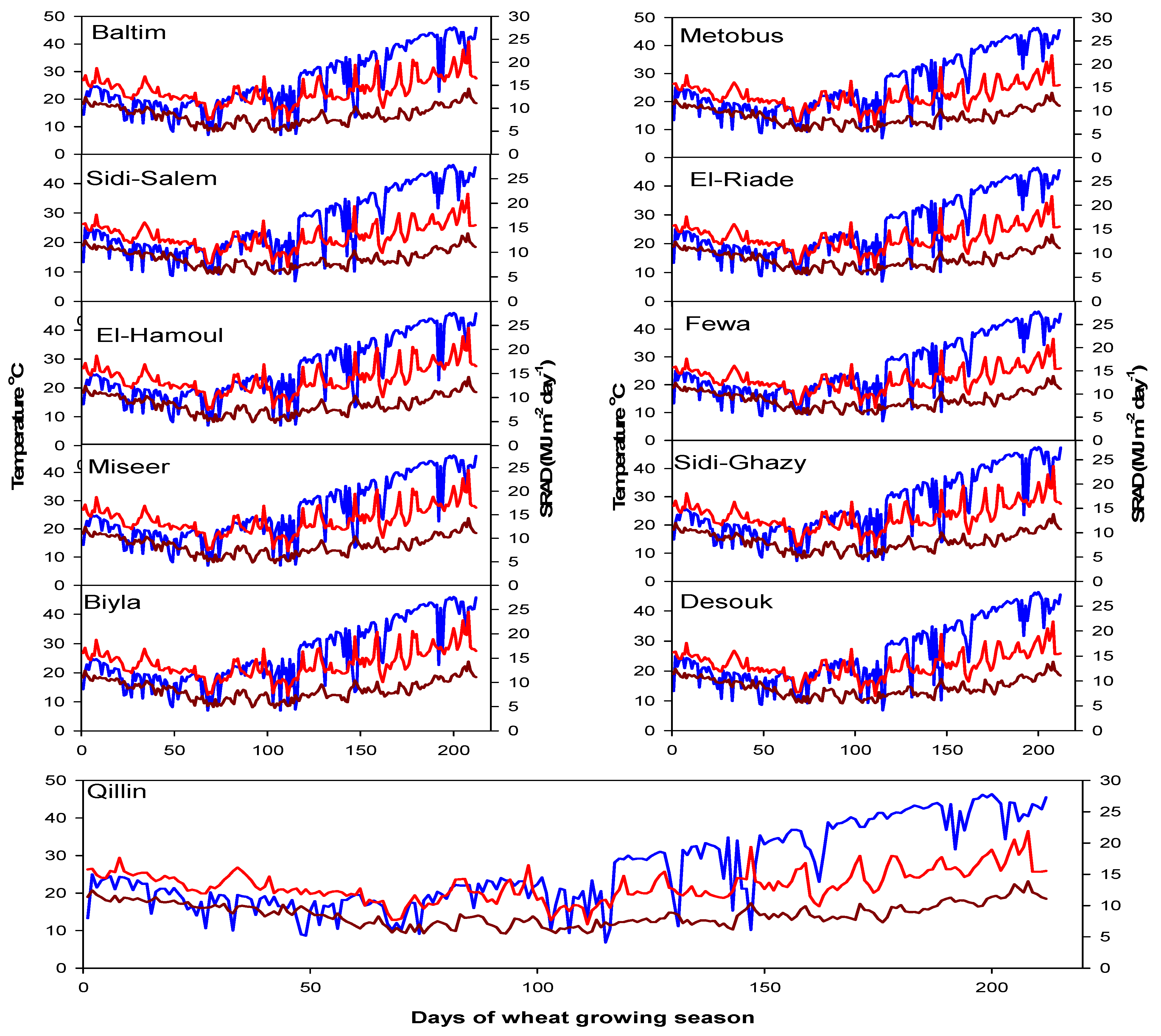
2.3. Weather Data Set

Data of daily temperatures and solar radiation were obtained from an automated weather station in Sakha Agricultural Research Station (Figure S2). The Sakha region is located in the first agro-climatic zone in Egypt with a thermic soil temperature regime and a torric soil moisture regime according to the USDA [36]. The required weather data for the other eleven districts in the Kafr El Sheikh Governorate are necessary for model predictions generated from the NASA website (https://power.larc.nasa.gov/, accessed on 5 October 2019) based on their coordinates (Figure 1).

2.4. Water Measurements

Soil moisture content was monitored daily using the time domain reflectometry (TDR) probes [37]. WP is used to define the relationship between crop production and the amount of water involved in crop production [38], and it is calculated using the following equation.
WP = GY AW
where WP is the water productivity of the grain yield (kg m–3), GY is the attainable grain yield (kg ha–1), and AW is the applied irrigation water (m3 ha–1).
Irrigation application efficiency is defined as the ratio between water consumed by the plant during the growing season (evapotranspiration) except for adequate rainfall and irrigation water applied and calculated using the following equation.
IAE = RWS AW × 100
where IAE is the irrigation application efficiency, and RWS is the stored water in the root zone.

2.5. Descriptions of AQUACROP and APSIM

The AQUACROP model, developed by FAO’s Land and Water Division, is a water-driven model that can be used for planning and scenario analysis [39,40]. The AQUACROP model connects its soil–crop–atmosphere components via its soil and water balance [41]. Climate file (minimum and maximum air temperatures, ETo, rainfall, and CO2), crop file (time to emergence, maximum canopy cover, start of senescence, and maturity), soil file, management file, irrigation file, and initial soil water conditions are among the six input files used in the simulation. The AQUACROP model calculates plant transpiration (Tr) and soil evaporation using canopy cover (CC) rather than leaf area index (LAI). Tr is proportional to the area of soil uncovered, whereas evaporation is proportional to the extent of soil cover (1-CC) [41]. The CC is calculated using daily transpiration and some key physiological characteristics of the crop such as leaf expansion, canopy development, and senescence. Water stress’s effects on canopy senescence, stomatal control (gs) of transpiration, and leaf growth are measured using indicators that range from 0 to 1. For a given climate and crop, the normalized crop water productivity (WP) is set between 15 and 20 g m2 for C3 crops and between 30 and 35 g m2 for C4 crops (Steduto et al., 2009). The model’s WP parameter is normalized to make it applicable to a wide range of locations and seasons including future climate scenarios [41]. The product of biomass (B) and harvest index (H) is used to calculate crop yield (GY) and harvest index (HI). The latter is represented by a linear increase over time, beginning with flowering and ending with physiological maturity. The AQUACROP model’s parameters were measured or estimated using experimental data; some were based on field experience and others used the model’s default values, regardless of the year [42].
The Agricultural Production Systems Simulator is a software tool that allows you to link sub-models (or modules) together to simulate agricultural systems [43]. Using a CERES-Wheat approach, the APSIM-Wheat module simulates the growth and development of a wheat crop in a daily time step on an area basis (per square meter, not per single plant). Weather (radiation, temperature), soil water and nitrogen, and management practices all influence wheat growth and development [44]. From emergence to terminal spikelet, APSIM-Wheat has eleven phasing development stages determined by the accumulation of thermal time and other factors such as vernalization, photoperiod, and nitrogen [45]. The length of each phase is determined by the fixed thermal time specified as tt _phase name>.wheat.xml. Daily biomass accumulation (DQ) is calculated by radiation interception (DQr), which is limited by soil water deficiency. The DQr is made up of intercepted radiation (IR), radiation use efficiency (RUE), diffuse factor (fd), stress factor (fs), and CO2 factor (fc). The leaf area index (LAI, m2 m2) and the extinction coefficient (K) are used to calculate radiation interception (I). In APSIM, the soil module includes the Soil N module, which describes the carbon and nitrogen dynamics in soil. The biom pool contains the more labile soil microbial biomass and microbial products, whereas the hum pool contains the rest of the soil organic matter.

2.6. Models’ Calibration and Evaluation

Both models were calibrated using field data set from 2019/2020 and validated using data set from the 2020/2021 growing season. Various parameters affecting CC, evapotranspiration (ET), total water content (TWC), and GY in AQUACROP were calibrated using measurements and simulation results. In AQUACROP, determining the initial canopy cover (CC0), which is dependent on the seed rate, the estimated weight, and the estimated germination rate, is the first step. The CC0 is also affected by the density of the plants and the size of the seedling’s initial canopy. The model calculates this parameter automatically. After determining some phenological dates, such as the dates after sowing, emergence, maximum canopy cover (CCx), senescence, and maturity, the model automatically estimated canopy expansion rates. The canopy growth coefficient (CGC), canopy decline coefficient (CDC), leaf expansion, and early senescence are the most important parameters for calibrating the CC. To accurately estimate the canopy cover, the water stress parameters and curve shapes were also adjusted (Table 2). Because heat units, which are expressed as growing degree days (GDDs) in the AQUACROP model, are important for crop development, determining the cumulative growing degree day (CGDD) in each crop development stage is interesting. The GDD is calculated in the AQUACROP model using the base temperature (Tbase) and the upper temperature (Tupper) (Table 2). These two temperatures are primarily determined by climate and wheat variety. AQUACROP manually uses 0 and 26 °C for Tbase and Tupper, respectively [46]. Many studies, however, used different values for Tbase and Tupper when testing the AQUACROP model for wheat. In our study, we used 5.0 and 35 °C for Tbase and Tupper, respectively, which are adapted to Egyptian climatic conditions and the current wheat variety (Table 2). Four stages characterized canopy development in AQUACROP including from sowing to emergence (Emrg), to maximum canopy cover (MaxCC), to senescence (Senc) and from sowing to maturity (Mat). The different thresholds characterizing these processes are defined in the AQUACROP model as the parameters related to water stress that affect leaf expansion, stomata conductance, and accelerated canopy senescence. The fractional depletion (p) of the total available water in the root zone is used to calculate these thresholds (TAW) (Table 2). The calibration of ETc was primarily based on determining the appropriate values of crop coefficients: maximum soil evaporation (Kex) for soil evaporation calculations and maximum crop transpiration coefficient (KcTr,x) for plant transpiration calculations. Finally, in the absence of local values for the reference harvest index (HIo) and normalized crop water productivity (WP*), these two parameters were calibrated using measured evapotranspiration and grain yield for the Sakha 95 variety.
The vernalization sensitivity (Vern_Sens), photoperiod sensitivity (Photo_Sens), thermal time needed from sowing to end of juvenile (tt_end_of_juvenile), thermal time needed in anthesis phase (tt_flowering), thermal time from the start of grain filling to maturity (tt_floral_initiation), thermal time from the start of grain filling to maturity (tt_start_grain_fill ), maximum grain size (Max_grain_size), grain growth rate from flowering to grain filling (potential_grain_growth_rate), potential daily grain filling rate(potential_grain_filling rate), and grain number per stem weight at the start of grain filling (grains_per_gram_stem) coefficients are used in the growth and development module of APSIM-Wheat to define phenology, crop growth, and yield in the time domain (Table 3). The cultivar coefficients were obtained in stages for calibration, starting with phenological development and then moving on to grain developmental parameters. The genetic coefficients were determined using the manual trial and error method. The values were adjusted so that the root mean square error (RMSE) between the simulated and observed data was as small as possible. Model performance was measured using the anthesis, physiological maturity date, LAI, biomass, and yield. The validation used the same values for this set of parameters to assess the performance and robustness of APSIM-Wheat.
The models were calibrated and evaluated with the Sakha 95 wheat cultivar in the current study. The calibration was carried out by selecting the best set of parameters in each specific model. The goodness of fit of such models were conducted using the coefficient of determination (R2), root means square deviation (RMSD), and model index of agreement (d) as was explained in [47,48,49].

2.7. Models Application

In the current research, two crop-based simulation models (i.e., AQUACROP and APSIM-Wheat) were used [14]. They were selected because they are widely used and well accepted in the crop modeling community [50]. Nevertheless, they have not been seen or tested in an agronomic field trial of wheat under Egyptian climate conditions. These models have mainly been used to extend the results for other locations in the same agro-climatic zone. Moreover, they are used to simulate different N and irrigation scenarios. Following model evaluation over two growing seasons, we applied different scenarios to predict the best water and N application practices to achieve higher grain yield values and WP. Scenarios included the following wide options (0.5, 0.6, 0.7, 0.8, 0.9, 1.0, 1.1, 1.2, 1.3, 1.4, and 1.5 ETc) of the required crop water and (50%, 60%, 70%, 80%, 90%, 100%, 110%, and 120% from the recommended N fertilizer dose). After calibration and application of both models, they can be valid tools to predict wheat yield for the agricultural districts in the Kafr El Sheikh Governorate.

3. Results and Discussion

3.1. Observed Wheat Yield, Phenology, Water Productivity, and Water Relations

As shown in Figures S3 and S4, values of wheat grain yield and final biomass were higher under optimum planting date, P2 (November 15th), N1, and I2. The highest grain yield obtained was 8.1 t ha−1 achieving an increase of 55 % compared with the lowest grain yield 3.7 t ha−1 under early planting date (P1), deficit irrigation (I3) and without N fertilizer application (N0), (Figure S4). The final biomass also increased with optimum planting date (P2), fertilization (N1) and irrigation regime (I2), achieving 16.5 t ha–1. Meanwhile, the lowest value 7.9 t ha–1 was noticed using lately planting date (P3), a deficit irrigation regime (I3), and N0 (Figure S4). The higher yield under P2 was mainly due to the environmental conditions, particularly temperature through the sensitive growth stage [43]. On the other hand, the lowest yield was noticed under P1 (the first planting date, November 10th) without any additions of N fertilizers as well as under extra irrigation (1.5 ETc). The increased wheat yields was an indicator of the vital role of N and compost in plant life and the contribution of cell division and elongation. Statistical analysis (Table S4) showed the high significant effects of different treatments on wheat yield.
The phenological development of wheat from emergence passing by flowering to maturity is mainly affected by temperature, day length, and potential physiological stresses [51,52]. Optimum planting date (P2), irrigation (I2), and fertilization (N1) achieved the highest value of anthesis (115 days) and maturity (144 days) as shown in Figures S5 and S6, respectively. This was mainly attributed to the decreasing mean temperature at these specific growth stages. Meanwhile, the lowest values were observed at 105 and 128 days for anthesis and maturity, respectively, under the first planting date (P1), the third irrigation treatment (I3), and N0.
Increasing the yield in wheat under the optimum planting date, irrigation, and fertilization was mainly due to the optimum environmental conditions, N fertilization for cell division and elongation, and the specific role of compost on increasing soil available water. Under P2, the values of available N after harvest and N uptake by whole plants were higher than those in P1 and P3 (Figures S7 and S8). In the same case, errors as the standard deviation in P2 were lower than those under P1 and P3 (Figures S3–S6).
Referring to the contribution of compost on mineralization rates and the actual contribution of compost on N availability, data in Figure S9A show that each one ton of compost can add about 0.7 kg of mineral N. This value had been already deducted from the initial analysis of compost (Table S3), where the available mineral N equal to 706 mg kg–1 of compost. Consequently, compost can add 10.5, 6.4, 8, and 9.7 kg N ha−1 for the following treatments N0, N1, N2, and N3. Such values have been already added, with those coming from mineral fertilizer (Figure S9B).
Currently, increasing crop WP is necessary due to the limited water resources and population increase [53,54]. The results showed that planting date, irrigation, and fertilization affected WP (Figure S10). The highest value of observed WP (1.6 kg m–3) was recorded under the second planting date (P2, the recommended), the second irrigation treatment (I2), and the first fertilizer treatment (N1). Meanwhile, the lowest value (0.7 kg m–3) was noticed under the first planting date, the third irrigation treatment, and N0 (Figure S10). This was mainly due to the increasing crop life period and, thus, increasing mean seasonal irrigation water applied (Figure S11A) under early planting date (P1) as well as decreasing yield due to the unsuitable environmental conditions. Different studies have shown that wheat can be grown with deficit irrigation without a significant yield reduction [55]. Similar to applied water, mean water use and water stored decreased with delaying planting dates from early to late. The highest water use and water stored values were 3591.9 and 3826.5 m3 ha–1, respectively, under the first planting date (Figure S11). These values decreased gradually under delayed planting dates. This was also a reason for decreasing WP in the case of the first planting date. Water application efficiency appeared in an opposite trend, where the highest value (73.5 %) was recorded under the third planting date (P3) and decreased to 67.8 % under the first planting date (P1) (Figure S11).

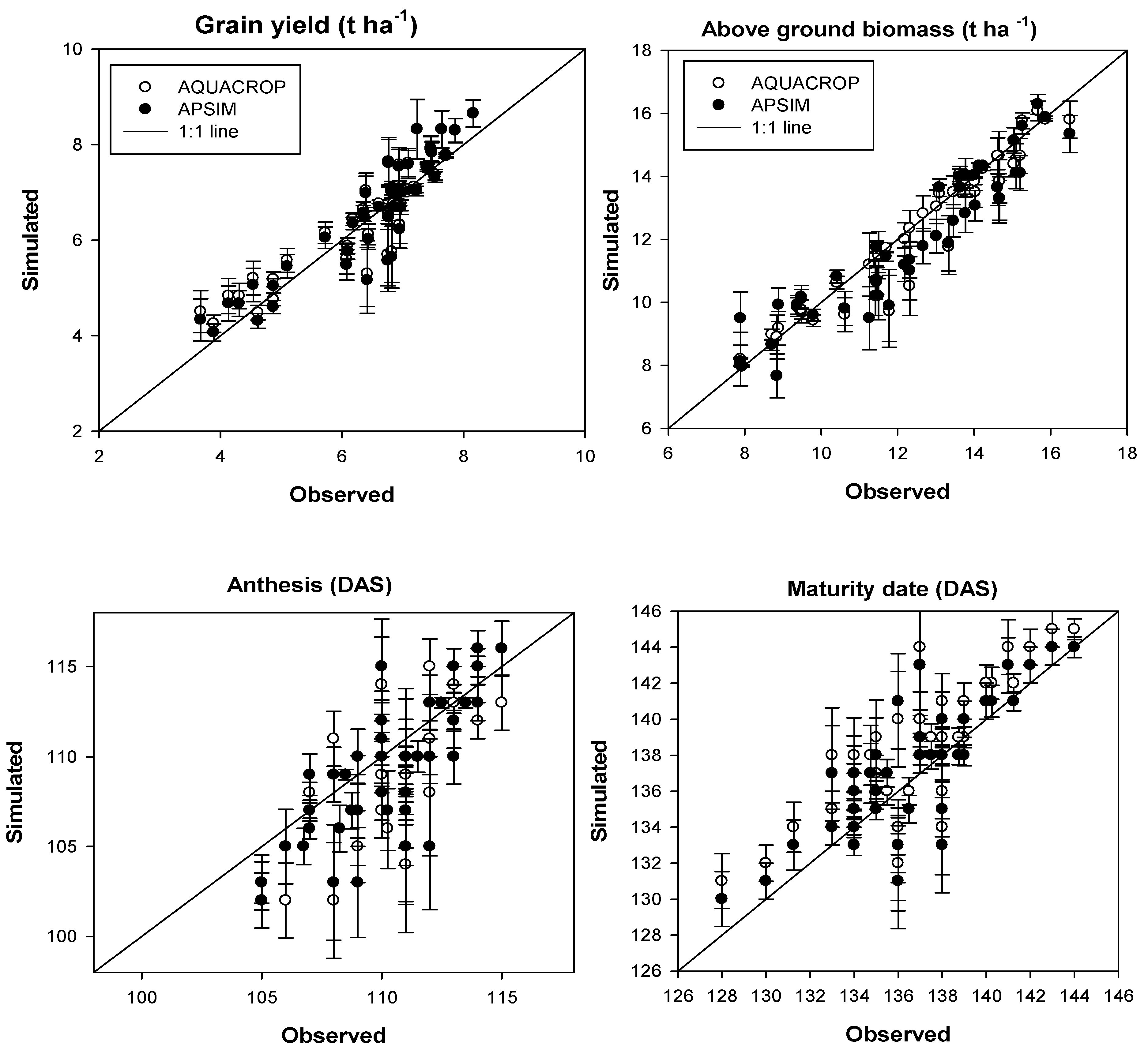
3.2. Model Calibrations

AQUACROP and APSIM-Wheat models were calibrated using the 2019/2020 and 2020/2021 successive seasons with the Sakha 95 genotype. The calibration included the tuning of specific parameters to match the field data set properties (N and yield) under all treatments. Table 2 and Table 3 supply the list of calibrated parameters for both models. The calibration process started first with phenology and followed by yield and biomass.
The genetic parameters determination, according to Godwin and Singh [16], were performed manually. The values were modified based on reaching the minimum RMSD between predicted and observed field data. It showed that the calibrations of AQUACROP and APSIM worked well and were very robust (Figure 2). The calibration of both models provided high agreement of grain yield, aboveground biomass, anthesis, and maturity dates. Both crop models reproduced grain yields well with an R2 = 0.84. In addition, RMSD values were 555 and 500 kg ha–1 with a high d of 0.93 and 0.94 for AQUACROP and APSIM, respectively (Table 2). The models showed a high predictive ability for yield under the current climatic conditions and management strategies. In addition, aboveground biomass simulations were predicted well using both models. Where R2 values of simulated biomass were 0.96 and 0.84, RMSD values were 309 and 613 kg ha–1. Moreover, the d values were 0.99 and 0.97 for both AQUACROP and APSIM wheat, respectively (Table 4). Regarding the simulations of wheat phenology (anthesis and maturity), plotted data in Figure 2 and statistical indicators in Table 4 showed a good agreement between simulated and observed values. Therefore, this study’s outcomes from the AQUACROP and APSIM-Wheat models could be used successfully as a decision support tool to select the fit cultivars.
It is well known that wheat phenology has a high impact on yield growth and development [56]. Anthesis and maturity dates were simulated well by both models (Figure 2 and Table 4). In APSIM-Wheat, the anthesis date was calibrated using Vern_Sens and Photo_Sens. Meanwhile, maturity date was controlled by tt_end_of_juvenile (Table 3). Therefore, we usually need to use these parameters for APSIM calibration [26,57]. While in the case of AQUACROP, anthesis and maturity dates could be modified and controlled by the time to flowering and time to maturity (Table 2). Accurate phenology stages are considered the first priority for model calibration [58]. Following robust calibrations and achieving less uncertainty, the model became ready to simulate yield and crop development accurately [59]. Solar radiation interception (RI) and RUE are considered the key factors of biomass production. Our findings showed a high accuracy in predicting aboveground biomass similar to that achieved by Arora et al. [60]. Because of the positive correlation between grain and biomass yields [61], biomass showed robust predictions. Here, biomass in APSIM-Wheat was determined using tt_floral_initiation (Table 3); meanwhile, in AQUACROP, it was controlled by plant density and maximum canopy cover (Table 2).
The tested models achieved a high robustness in yield predictions. In APSIM-Wheat, the parameters responsible for determining grain yield are grain growth rate, maximum grain size, and potential grain filling rate (Table 3). Meanwhile, in the case of AQUACROP, harvest index is the required parameter for grain yield calibration. Therefore, by modifying these parameters, the grain yield of the specific cultivar can be increased or decreased, provided that it must be modified after the crop phenology calibration [62].

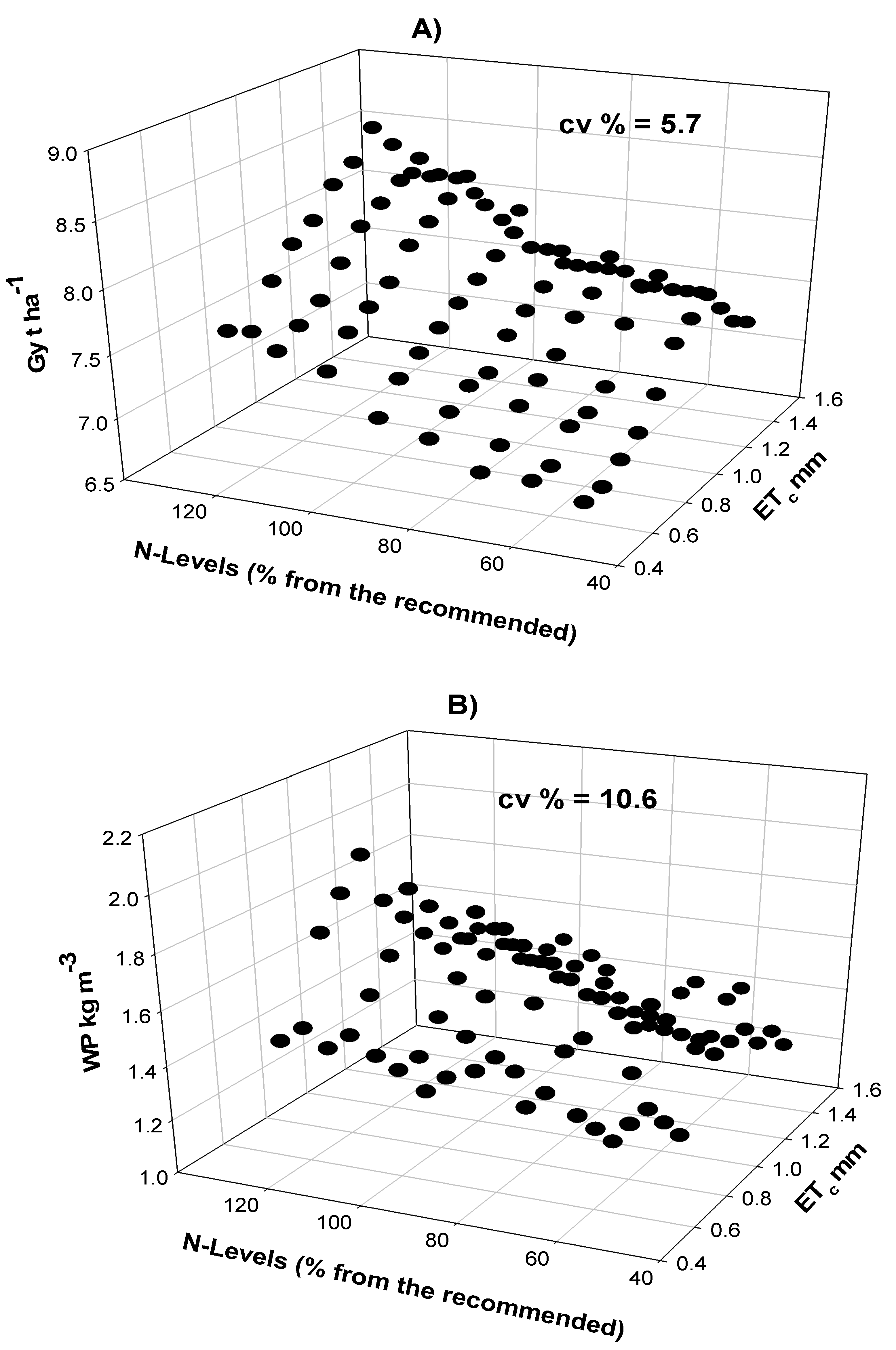
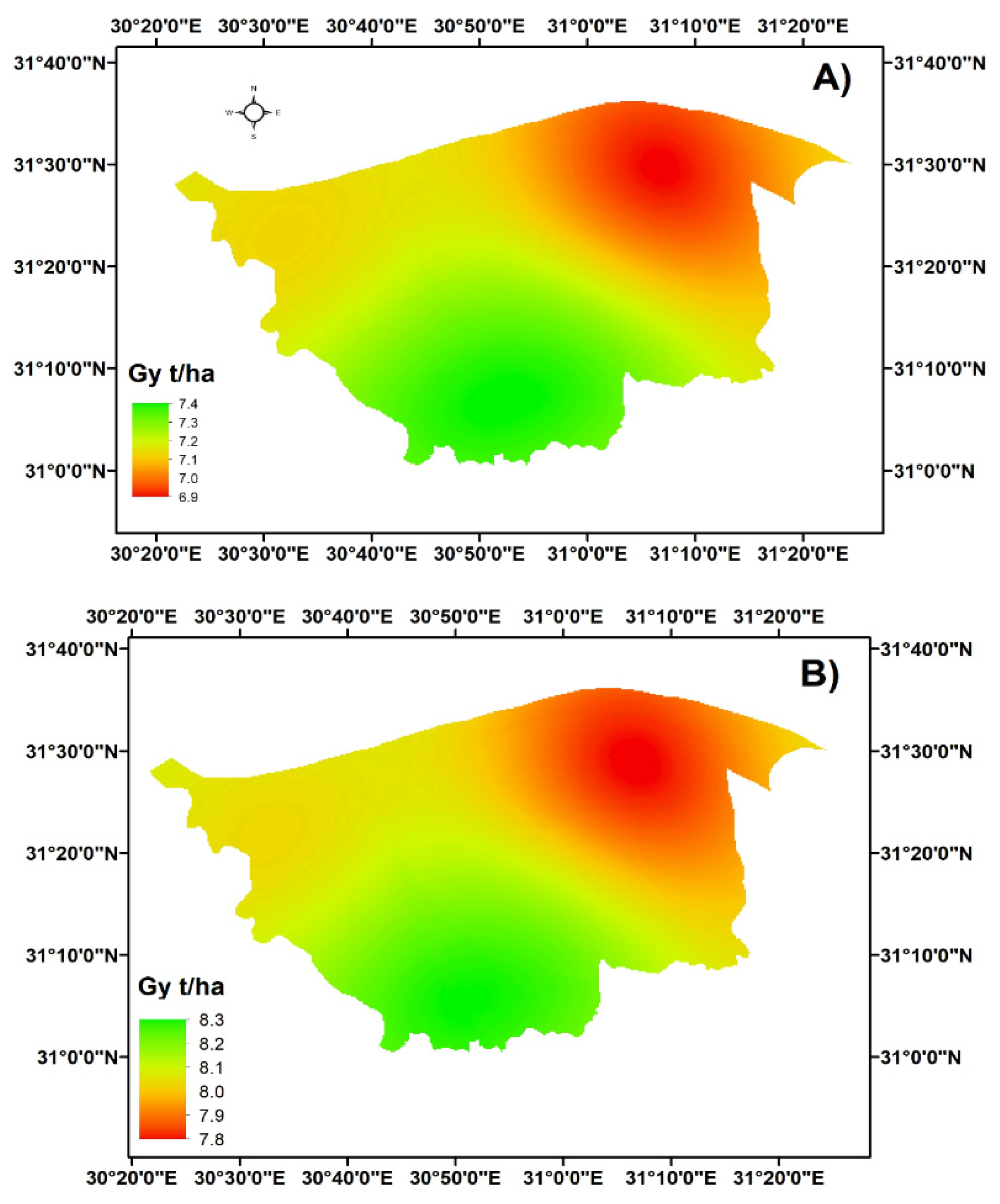
3.3. Model Applications

After model calibrations using various experimental data sets in the studied area, we used both models to predict grain yield and WP in response to various options of N and water as treatment inputs in crop models. This was conducted to determine which scenario could maximize yield and WP. The data in Figure 3A,B show the predicted wheat yield and WP, respectively, under various scenarios of water regime and N fertilizer doses. The data show that the highest yield of 8.7 t ha−1 was predicted under 120% from recommended N in combination with irrigation by 1.2 ETc (Figure 3A). Meanwhile, the highest value of WP 2.0 kg m–3 was noticed under 120% from recommended N with deficit irrigation 0.8 ETc (Figure 3B). In addition, it is necessary and important to observe that the WP value under irrigation 100% from the actual evapotranspiration (1.0 ETc) and 100% from the recommended N fertilizer, 1.8 kg m–3 was quite like that obtained under (120%) N and a deficit irrigation (0.7 ETc) (Figure 3B). It was also noticed from the model simulations that a wheat productivity of 7.4 t ha–1 could be obtained by adding 80% from recommended doses of N fertilizer and 1.2 ETc as irrigation water applied. At this point, WP would be 1.5 kg m–3. In arid and semi-arid climate regions such as Egypt, where water resources are limited, deficit irrigations can produce satisfactory and substantial yields of wheat fertilized with suitable N application. This study’s findings showed an increase in WP under deficit irrigation.
In conclusion, a combination of a lower quantity of water applied and appropriate management of N fertilizer will increase wheat WP in the region. In addition, we recommend two management practices used in this study that can enhance wheat yield and WP. The first recommendation, which resulted from two growing seasons (i.e., field experiments), concludeds that N1 (100% of the recommended N combined with 9.0 t ha–1 compost) and I2 (1.0 ETc) gave the highest yield and WP. Meanwhile, the second recommendation, extracted from different predicted water and N management scenarios, suggest using (120% of the recommended N) in combination with 0.8 ETc gave the highest value of WP as predicted by both crop models. The first recommended treatment gave 8.2 t ha–1 of grain yield and 1.6 kg m–3 for WP. Meanwhile, the second set of treatment increased the yield to 8.5 t ha–1 and a sharp increase in WP to 2.0 kg m–3. Therefore, we have used the previous two main recommendations separately to predict wheat yield in all districts (11 sites) of the governorate (Figure 4A,B; Table 5). Based on the World Reference Base for Soil Resources, the principal leading soil group is Fluvisols (Fl) with central primary texture clay and loamy clay [63,64]. Meanwhile, climatic data for all locations were generated from NASA’s AgCFSR climate data set (http://data.giss.nasa.gov/impacts/agmipcf/, accessed on 1 December 2021) and used for simulations (Figure 3). The overall wheat yields, as predicted by two crop models using the first recommended treatments (Figure 4A), were slightly lower than that predicted by the second recommended treatments (Figure 4B). This was mainly attributed to increasing the N fertilizer dose in the second scenario (i.e., 120% of the recommended), which equaled 144 kg N ha–1, and its role in maximizing the yield and irrigation with 0.8 ETc. Meanwhile, the first recommended treatments indicated that by adding 100% of the recommended N combined with 9.2 t ha–1 from compost, achieved 126.4 kg N ha–1 with irrigation at 1.0 ETc. The studied districts that already cover the agricultural area in Kafr El Sheikh included Baltim, El-Hamoul, Metrobus, El-Riad, Sidi Salem, Sidi Ghazy, Fewa, Biyala, Desouk, Miseer and Qillin. As demonstrated in Figure 4A,B, wheat yield decreased in the north, while it increased towards in the southern direction. However, temperature increased in a southern trend. This was mainly attributed to increasing soil salinity resulting from sea water intrusion into locations close to the Mediterranean Sea (Figure S1B). Therefore, AQUACROP and APSIM-Wheat predicted the yield and maximized its value in the North Delta of Egypt successfully.

4. Conclusions

Wheat production in regions suffering from limited water resources, such as Egypt, is faced by deficits in irrigation and N fertilization. In this study, APSIM-Wheat and AQUACROP showed high accuracy in simulating anthesis date, maturity date, grain yield, and aboveground biomass. Statistical indicators, including R2, RMSD, and d confirmed such accuracy for both models. These models were used to predict yield and agricultural WP under various treatments of irrigation and N fertilization. When compared to grain yield, WP generally decreased as applied water increased. The conducted field experiments over two successive growing seasons demonstrated that the highest WP (1.6 kg m–3) was achieved under the recommended planting date (P2), the recommended N fertilizer combined with 9.2 t ha–1 of compost (N1) as well as using the actual evapotranspiration 1.0 ETC as applied irrigation water (I2). Different irrigation and nitrogen fertilization scenarios were used as model inputs to explore the best option achieving the maximum WP.
Consequently, the highest value of WP 2.0 kg m–3 was predicted by using 120% of the recommended N and 0.8 ETc as water application. Importantly, under all scenarios of used irrigation and fertilization, the WP ranged from 1.7 to 2.0 kg m–3, meanwhile grain yield ranged from 6.8 to 8.7 t ha–1. This wide range was mainly attributed to the interaction effects of irrigation and fertilization on yield and WP. Noticeably, farmers’ yield in the North Delta of Egypt of 7.4 t ha–1 was predicted by adding 80% of the recommended N and 1.4 ETc as irrigation water, which resulted in the lower value of WP 1.5 kg m–3. The APSIM-Wheat and AQUACROP models can be used to predict and optimize wheat yield and water productivity under different irrigation and fertilization treatments in Egypt.

Supplementary Materials

The following are available online at https://www.mdpi.com/article/10.3390/land10121375/s1, Figure S1. Map of the studied area at River Nile North delta, Kafr El- Sheikh Governorate (A) and its soil salinity of the effective root zone (B); Figure S2. Daily maximum and minimum temperature (°C) and solar radiation (MJ m−2 day−1) data of Sakha as average of two growing seasons 2014/2015 and 2015/2016; Figure S3. Wheat grain yield as affected by irrigation, fertilization and planting dates (data represent the average of both seasons); Figure S4. Final above ground biomass of wheat (t ha−1) as affected by irrigation, fertilization and planting dates, (data represent the average of both seasons); Figure S5. Anthesis date (DAS) as affected by irrigation, fertilization and planting dates (data represent the average of both seasons); Figure S6. Maturity date (DAS) as affected by irrigation, fertilization and planting dates (data represent the average of both seasons); Figure S7. Soil available mineral N remained in soil after wheat crop harvest (data represent the average of both seasons); Figure S8. Total N uptake in whole wheat under different treatments (data represent the average of both seasons); Figure S9. The added mineral N to the soil from compost (A) and both compost and mineral nitrogen fertilization (B) under different treatments; Figure S10. Effects of irrigation, fertilization, and planting dates on Wheat WP (data represent the average of both seasons); Figure S11. Wheat water applied (a), use (b), stored(c) and application efficiency (d) as affected by irrigation and planting dates; Table S1 Soil physical properties of the studied soils before treatment application; Table S2 Soil chemical properties of the studied soils before treatment application; Table S3 The detailed chemical and nutritional analysis of the used compost, according to [28]; Table S4 Main effects of planting dates, irrigation and fertilization on wheat grain and biomass yields (data represent the average of two seasons).

Author Contributions

Conceptualization, A.M.S.K., M.F.S. and H.M.A.; methodology, A.A., M.G.Z., M.M.A.S. and H.A.; software, A.M.S.K., M.F.S., H.M.A. and A.M.A.-S.; formal analysis, A.M.S.K. and M.F.S., investigation, A.M.S.K., A.M.A.-S., H.M.A. and H.A.; resources, A.M.S.K., M.F.S. and A.A.; data curation, C.S., M.F.S., A.M.A.-S., H.A. and H.M.A.; writing—original draft preparation, A.M.S.K., K.A.A. and M.F.S.; writing—review and editing, all authors. All authors have read and agreed to the published version of the manuscript.

Funding

This research was funded by Researchers Supporting Project (number: RSP-2021/334), King Saud University, Riyadh, Saudi Arabia.

Data Availability Statement

All data are presented within the article and Supplementary Materials.

Acknowledgments

The authors extend their appreciation to the Researchers Supporting Project (number: RSP-2021/334), King Saud University, Riyadh, Saudi Arabia.

Conflicts of Interest

The authors declare no conflict of interest.

References

  1. Seleiman, M.F.; Kheir, A.M.S.; Al-Dhumri, S.; Alghamdi, A.G.; Omar, E.-S.H.; Aboelsoud, H.M.; Abdella, K.A.; Abou El Hassan, W.H. Exploring Optimal Tillage Improved Soil Characteristics and Productivity of Wheat Irrigated with Different Water Qualities. Agronomy 2019, 9, 233. [Google Scholar] [CrossRef] [Green Version]
  2. Asseng, S.; Kheir, A.M.S.; Kassie, B.T.; Hoogenboom, G.; Abdelaal, A.I.N.; Haman, D.Z.; Ruane, A.C. Can Egypt become self-sufficient in wheat? Environ. Res. Lett. 2018, 13, 094012. [Google Scholar] [CrossRef] [Green Version]
  3. Ding, Z.; Kheir, A.M.S.; Ali, O.A.M.; Hafez, E.M.; ElShamey, E.A.; Zhou, Z.; Wang, B.; Lin, X.; Ge, Y.; Fahmy, A.E.; et al. A vermicompost and deep tillage system to improve saline-sodic soil quality and wheat productivity. J. Environ. Manag. 2021, 277, 111388. [Google Scholar] [CrossRef] [PubMed]
  4. Ding, Z.; Ali, E.F.; Aldhumri, S.A.; Ghoneim, A.M.; Kheir, A.M.S.; Ali, M.G.M.; Eissa, M.A. Effect of Amount of Irrigation and Type of P Fertilizer on Potato Yield and NH3 Volatilization from Alkaline Sandy Soils. J. Soil Sci. Plant Nutr. 2021, 21, 1565–1576. [Google Scholar] [CrossRef]
  5. Roy, R.; Núez-Delgado, A.; Sultana, S.; Wang, J.; Mmunirf, A.; Battaglia, M.; Sarker, T.; Seleiman, M.F.; Barmon, M.; Zhang, R.Q. Additions of optimum water, spent mushroom compost and wood biochar to improve the growth performance of althaea rosea in drought-prone coal-mined spoils. J. Environ. Manag. 2021, 295, 113076. [Google Scholar] [CrossRef] [PubMed]
  6. Sullivan, D.; Bary, A.; Nartea, T.; Myrhe, E.; Cogger, C.; Fransen, S.N. itrogen availability seven years after a high-rate food waste compost application. Compos. Sci. Util. 2003, 11, 265–275. [Google Scholar] [CrossRef]
  7. Hargreaves, J.; Adl, M.; Warman, P.A. Areview of the use of composted municipal solid waste in agriculture. Agric. Ecosyst. Environ. 2008, 123, 1–14. [Google Scholar] [CrossRef]
  8. Ding, Z.; Ali, E.F.; Elmahdy, A.M.; Ragab, K.E.; Seleiman, M.F.; Kheir, A.M.S. Modeling the combined impacts of deficit irrigation, rising temperature and compost application on wheat yield and water productivity. Agric. Water Manag. 2021, 244, 106626. [Google Scholar] [CrossRef]
  9. Prasad, M.A. Literature Review on the Availability of Nitrogen from Compost in Relation to the Nitrate Regulations; Environment Protection Agency: Wexford, Ireland, 2009; p. 378. [Google Scholar]
  10. Franklin, D.; Bender-Özenç, D.; Özenç, N.; Cabrera, M. Nitrogen mineralization and phosphorus release from composts and soil conditioners found in the Southeastern United States. Soil Sci. Soc. Am. J. 2015, 79, 1386–1395. [Google Scholar] [CrossRef]
  11. Alkharabsheh, H.M.; Seleiman, M.F.; Hewedy, O.A.; Battaglia, M.L.; Jalal, R.S.; Alhammad, B.A.; Schillaci, C.; Ali, N.; Al-Doss, A. Field Crop Responses and Management Strategies to Mitigate Soil Salinity in Modern Agriculture: A Review. Agronomy 2021, 11, 2299. [Google Scholar] [CrossRef]
  12. Dong, C.; Hu, D.; Fu, Y.; Wang, M.; Liu, H. Analysis and optimization of the effect of light and nutrient solution on wheat growth and development using an inverse system model strategy. Comput. Electr. Agric. 2014, 109, 221–231. [Google Scholar] [CrossRef]
  13. Donatelli, M.; Van Ittersum, M.K.; Bindi, M.; Porter, J.R. Modelling cropping systems-highlights of the symposium and preface to the special issues. Eur. J. Agron. 2002, 18, 1–11. [Google Scholar] [CrossRef]
  14. Keating, B.A.; Carberry, P.S.; Hammer, G.L.; Probert, M.E.; Robertson, M.J.; Holzworth, D.; Huth, N.I.; Hargreaves, J.N.G.; Meinke, H.; Hochman, Z.; et al. An overview of APSIM: A model designed for farming systems simulation. Eur. J. Agron 2003, 18, 267–288. [Google Scholar] [CrossRef] [Green Version]
  15. Ritchie, J.T.; Singh, U.; Godwin, D.; Bowen, W.T. Cereal growth, development, and yield. In Understanding Options for Agricultural Production; Tsuji, G.Y., Hoogenboom, G., Thornton, P.K., Eds.; Kluwer Academic: Dordrecht, The Netherlands, 1998; pp. 79–98. [Google Scholar]
  16. Godwin, D.C.; Singh, U. Nitrogen balance and crop response to nitrogen in upland and lowland cropping systems. In Understanding Options for Agricultural Production; Tsuji, G., Hoogenboom, G., Thornton, P., Eds.; Springer: Dordrecht, The Netherlands, 1998; pp. 55–77. [Google Scholar]
  17. Basso, B.; Liu, L.; Ritchie, J.T. A comprehensive review of the CERES-Wheat, -Maize and -Rice models’ performances. In Advances in Agronomy; Donald, L.S., Ed.; 2016; Volume 136, pp. 27–132. Available online: https://www.sciencedirect.com/science/article/abs/pii/S0065211315001480?via%3Dihub (accessed on 6 December 2021).
  18. Jones, J.W.; Hoogenboom, G.; Porter, C.H.; Boote, K.J.; Batchelor, W.D.; Hunt, L.A.; Wilkens, P.W.; Singh, U.; Gijsman, A.J.; Ritchie, J.T. The DSSAT cropping system model? Eur. J. Agron. 2003, 18, 235–265. [Google Scholar] [CrossRef]
  19. Kheir, A.M.S.; El Baroudy, A.; Aiad, M.A.; Zoghdan, M.G.; Abd El-Aziz, M.A.; Ali, M.G.M.; Fullen, M.A. Impacts of rising temperature, carbon dioxide concentration and sea level on wheat production in North Nile delta. Sci. Total Environ. 2019, 651, 3161–3173. [Google Scholar] [CrossRef]
  20. Wang, X.C.; Li, J.; Tahir, M.N.; Fang, X.Y. Validation of the EPIC model and its utilization to research the sustainable recovery of soil desiccation after alfalfa (Medicago sativa L.) by grain crop rotation system in the semi-humid region of the Loess Plateau. Agric. Ecosyst. Environ. 2012, 161, 152–160. [Google Scholar] [CrossRef]
  21. Brisson, N.; Gary, C.; Justes, E.; Roche, R.; Mary, B.; Ripoche, D.; Zimmer, D.; Sierra, J.; Bertuzzi, P.; Burger, P.; et al. An overview of the crop model STICS. Eur. J. Agron. 2003, 18, 309–332. [Google Scholar] [CrossRef]
  22. Martre, P.; Wallach, D.; Asseng, S.; Ewert, F.; Jones, J.W.; Rötter, R.P.; Boote, K.J.; Ruane, A.C.; Thorburn, P.J.; Cammarano, D.; et al. Multimodel ensembles of wheat growth: Many models are better than one. Glob. Chang. Biol. 2015, 21, 911–925. [Google Scholar] [CrossRef] [PubMed]
  23. Ali, M.G.M.; Ibrahim, M.M.; El Baroudy, A.; Fullen, M.; Omar, E.-S.H.; Ding, Z.; Kheir, A.M.S. Climate change impact and adaptation on wheat yield, water use and water use efficiency at North Nile Delta. Front. Earth Sci. 2020, 14, 522–536. [Google Scholar] [CrossRef]
  24. Kheir, A.M.S.; Alrajhi, A.A.; Ghoneim, A.M.; Ali, E.F.; Magrashi, A.; Zoghdan, M.G.; Abdelkhalik, S.A.M.; Fahmy, A.E.; Elnashar, A. Modeling deficit irrigation-based evapotranspiration optimizes wheat yield and water productivity in arid regions. Agric. Water Manag. 2021, 256, 107122. [Google Scholar] [CrossRef]
  25. Asseng, S.; Fillery, I.R.P.; Anderson, G.C.; Dolling, P.J.; Dunin, F.X.; Keating, B.A. Use of the APSIM wheat model to predict yield, drainage, and NO3—Leaching for a deep sand. Aust. J. Exp. Agric. 1998, 49, 363–378. [Google Scholar] [CrossRef]
  26. Asseng, S.; Keating, B.A.; Fillery, I.R.P.; Gregory, P.J.; Bowden, J.W.; Turner, N.C.; Palta, J.A.; Abrecht, D.G. Performance of the APSIM-wheat model in western australia. Field Crop. Res. 1998, 57, 163–179. [Google Scholar] [CrossRef]
  27. Wang, E.; van Oosterom, E.J.; Meinke, H.; Asseng, S.; Robertson, M.J.; Huth, N.I.; Keating, B.A.; Probert, M. The new APSIM-Wheat model: Performance and future improvements. In Proceedings of the 11th Australian Agronomy Conference, Geelong, Victoria, 2–6 February 2003; Unkovich, M., O’Leary, G., Eds.; Australian Society of Agronomy: Geelong, Australia, 2003. [Google Scholar]
  28. Asseng, S.; Jamieson, P.D.; Kimball, B.; Pinter, P.; Sayre, K.; Bowden, J.W.; Howden, S.M. Simulated wheat growth affected by rising temperature,increased water deficit and elevated atmospheric CO2. Field Crop. Res. 2004, 85, 85–102. [Google Scholar] [CrossRef]
  29. Steduto, P.; Hsiao, T.C.; Fereres, E.; Raes, D. Crop Yield Response to Water; FAO Irrigation and Drainage: Rome, Italy, 2012; p. 500. [Google Scholar]
  30. Khoshravesh, M.; Mostafazadeh-Fard, B.; Heidarpour, M.; Kiani, A.R. AquaCrop model simulation under different irrigation water and nitrogen strategies. Water Sci. Technol. 2013, 67, 232–238. [Google Scholar] [CrossRef] [PubMed]
  31. Paredes, P.; de Melo-Abreu, J.P.; Alves, I.; Pereira, L.S. Assessing the performance of the FAO AquaCrop model to estimate maize yields and water use under full and deficit irrigation with focus on model parameterization. Agric. Water Manag. 2014, 144, 81–97. [Google Scholar] [CrossRef] [Green Version]
  32. Mhizha, T.; Geerts, S.; Vanuytrecht, E.; Makarau, A.; Raes, D. Use of the FAO AquaCrop model in developing sowing guidelines for rainfed maize in Zimbabwe. Water SA 2014, 40, 233–244. [Google Scholar] [CrossRef] [Green Version]
  33. Kumar, P.; Sarangi, A.; Singh, D.K.; Parihar, S.S. Evaluation of AquaCrop model in predicting wheat yield and water productivity under irrigated saline regimes. Irrig. Drain. 2014, 63, 474–487. [Google Scholar] [CrossRef]
  34. Abdel Kawy, W.A.M.; Ali, R.R. Assessment of soil degradation and resilience at northeast Nile Delta, Egypt: The impact on soil productivity. Egypt. J. Remote Sens. Space Sci. 2012, 15, 19–30. [Google Scholar] [CrossRef] [Green Version]
  35. Klute, A. Methods of Soil Analysis. Part I-Physical and Mineralogical Methods, 2nd ed. 1986. Available online: https://acsess.onlinelibrary.wiley.com/doi/book/10.2136/sssabookser5.1.2ed (accessed on 6 December 2021).
  36. USDA. Keys to Soil Taxonomy, 3rd ed.; United State Department of Agriculture, Natural Resources Conservation Service (NRCS): Washington, DC, USA, 2010. [Google Scholar]
  37. Heimovaara, T.J.; Huisman, J.A.; Vrugt, J.A.; Bouten, W. Obtaining the spatial distribution of water content along a TDR probe using the SCEM-UA bayesian inverse modeling scheme. Vadose Zone J. 2004, 3, 128–145. [Google Scholar] [CrossRef]
  38. Ali, M.H.; Talukder, M.S.U. Increasing water productivity in crop production—Asynthesis. Agric. Water Manag. 2008, 95, 1201–1213. [Google Scholar] [CrossRef]
  39. Steduto, P.; Hsiao, T.C.; Raes, D.; Fereres, E. AquaCrop—The FAO Crop Model to Simulate Yield Response to Water: I. Concepts and Underlying Principles. Agron. J. 2009, 101, 426–437. [Google Scholar] [CrossRef] [Green Version]
  40. Hsiao, T.C.; Heng, L.; Steduto, P.; Rojas-Lara, B.; Raes, D.; Fereres, E. AquaCrop—The FAO Crop Model to Simulate Yield Response to Water: III. Parameterization and Testing for Maize. Agron. J. 2009, 101, 448–459. [Google Scholar] [CrossRef]
  41. Araya, A.; Habtu, S.; Hadgu, K.M.; Kebede, A.; Dejene, T. Test of AquaCrop model in simulating biomass and yield of water deficient and irrigated barley (Hordeum vulgare). Agric. Water Manag. 2010, 97, 1838–1846. [Google Scholar] [CrossRef]
  42. Iqbal, M.A.; Shen, Y.; Stricevic, R.; Pei, H.; Sun, H.; Amiri, E.; Penas, A.; del Rio, S. Evaluation of the FAO AquaCrop model for winter wheat on the North China Plain under deficit irrigation from field experiment to regional yield simulation. Agric. Water Manag. 2014, 135, 61–72. [Google Scholar] [CrossRef]
  43. Holzworth, D.P.; Huth, N.I.; deVoil, P.G.; Zurcher, E.J.; Herrmann, N.I.; McLean, G.; Chenu, K.; van Oosterom, E.J.; Snow, V.; Murphy, C.; et al. APSIM—Evolution towards a New Generation of Agricultural Systems Simulation. Environ. Model. Softw. 2014, 62, 327–350. [Google Scholar] [CrossRef]
  44. Zheng, B.; Chenu, K.; Doherty, A.; Chapman, S. The APSIM-Wheat Module (7.5 R3008). 2014, p. 615. Available online: https://scholar.google.com.au/citations?view_op=view_citation&hl=en&user=QtqjfIIAAAAJ&citation_for_view=QtqjfIIAAAAJ:5nxA0vEk-isC (accessed on 6 December 2021).
  45. Chen, C.; Wang, E.; Yu, Q. Modelling the effects of climate variability and water management on crop water productivity and water balance in the North China Plain. Agric. Water Manag. 2010, 97, 1175–1184. [Google Scholar] [CrossRef]
  46. Raes, D.; Steduto, P.; Hsiao, T.C.; Fereres, E. AquaCrop, Version 4.0. ReferenceManual; FAO, Land and Water Division: Rome, Italy, 2012; p. 130. [Google Scholar]
  47. Willmott, C.J. On the evaluation of model performance in physical geography. In Spatial Statistics and Models; Gaile, G.L., Willmott, C.J., Eds.; D. Reidel: Boston, MA, USA, 1984; pp. 443–460. [Google Scholar]
  48. Jacovides, C.P.; Kontoyiannis, H. Statistical procedures for the evaluation of evapotranspiration computing models. Agric. Water Manag. 1995, 27, 365–371. [Google Scholar] [CrossRef]
  49. Moriasi, D.N.; Arnold, J.G.; Liew, M.W.V.; Bingner, R.L.; Harmel, R.D.; Veith, T.L. Model evaluation guidelines for systematic quantification of accuracy in watershed simulations. Trans. ASABE 2007, 50, 885–900. [Google Scholar] [CrossRef]
  50. Tubiello, F.N.; Ewert, F. Simulating the effects of elevated CO2 on crops: Approaches and applications for climate change. Eur. J. Agron. 2002, 18, 57–74. [Google Scholar] [CrossRef]
  51. Asseng, S.; Ewert, F.; Martre, P.; Rotter, R.P.; Lobell, D.B.; Cammarano, D.; Kimball, B.A.; Ottman, M.J.; Wall, G.W.; White, J.W.; et al. Rising temperatures reduce global wheat production. Nat. Clim. Chang. 2015, 5, 143–147. [Google Scholar] [CrossRef]
  52. Olesen, J.E.; Børgesen, C.D.; Elsgaard, L.; Palosuo, T.; Rötter, R.P.; Skjelvåg, A.O.; Peltonen-Sainio, P.; Börjesson, T.; Trnka, M.; Ewert, F.; et al. Changes in time of sowing, flowering and maturity of cereals in Europe under climate change. Food Addit. Contam. Part A 2012, 29, 1527–1542. [Google Scholar] [CrossRef] [PubMed]
  53. Kijne, J.W.; Barker, R.; Molden, D. Water Productivity in Agriculture: Limits and Opportunities for Improvement; Comprehensive Assessment of Water Management in Agriculture, Series; No. 1 International Water Management Institute: Wallingford, UK; CABI: Colombo, Sri Lanka, 2003. [Google Scholar]
  54. Saad, A.M.; Mohamed, M.G.; El-Sanat, G.A. Evaluating AquaCrop model to improve crop water productivity at North Delta soils, Egypt. Adv. Appl. Sci. Res. 2014, 5, 293–304. [Google Scholar]
  55. Zhang, H.; Oweis, T.Y.; Garabet, S.; Pala, M. Water-use efficiency and transpiration efficiency of wheat under rain-fed conditions and supplemental irrigation in a Mediterranean-type environment. Plant Soil 1998, 201, 295–305. [Google Scholar] [CrossRef]
  56. Ceglar, A.C.; Repinšek, Z.; Kajfež-Bogataj, L.; Pogačar, T. The simulation of phenological development in dynamic crop model: The Bayesian comparison of different methods. Agric. For. Meteorol. 2011, 151, 101–115. [Google Scholar] [CrossRef]
  57. Ahmed, M.; Nasib, A.M.; Asim, M.; Aslam, M.; Ul-Hassan, F.; Higgins, S.; Stöckle, C.O.; Hoogenboom, G. Calibration and validation of APSIM-Wheat and CERES-Wheat for spring wheat under rainfed conditions: Models evaluation and application. Comput. Electron. Agric. 2016, 123, 384–401. [Google Scholar] [CrossRef]
  58. Archontoulis, S.V.; Miguez, F.E.; Moore, K.J. A methodology and an optimization tool to calibrate phenology of short-day species included in the APSIM PLANT model: Application to soybean. Environ. Modell. Softw. 2014, 62, 465–477. [Google Scholar] [CrossRef]
  59. Robertson, M.J.; Carberry, P.S.; Huth, N.I.; Turpin, J.E.; Probert, M.E.; Poulton, P.L.; Bell, M.; Wright, G.C.; Yeates, S.J.; Brinsmead, R.B. Simulation of growth and development of diverse legume species inAPSIM. Aust. J. Agric. Res. 2002, 53, 429–446. [Google Scholar] [CrossRef]
  60. Arora, V.K.; Singh, H.; Singh, B. Analyzing wheat productivity responses to climatic, irrigation and fertilizer-nitrogen regimes in a semi-arid sub-tropical environment using the CERES-Wheat model. Agric. Water Manag. 2007, 94, 22–30. [Google Scholar] [CrossRef]
  61. Dettori, M.; Cesaraccio, C.; Motroni, A.; Spano, D.; Duce, P. Using CERES-Wheat to simulate durum wheat production and phenology in Southern Sardinia. Field Crop. Res. 2011, 120, 179–188. [Google Scholar] [CrossRef]
  62. Ma, L.; Ahuja, L.R.; Saseendran, S.A.; Malone, R.W.; Green, T.R.; Nolan, B.T.; Bartling, P.N.S.; Flerchinger, G.N.; Boote, K.J.; Hoogenboom, G. A Protocol for Parameterization and Calibration of RZWQM2 in Field Research. Methods of Introducing System Models into Agricultural Research. Ahuja, L.R., Ma, L., Eds.; 2011, pp. 1–64. Available online: https://acsess.onlinelibrary.wiley.com/doi/abs/10.2134/advagricsystmodel2.c1 (accessed on 6 December 2021).
  63. Taha, M.H. Soil fertility management in Egypt. In Proceedings of the Regional Workshop on Soil Fertility Management through Farmer Field Schools in the Near East, Amman, Jordan, 14–16 December 1998; pp. 2–5. [Google Scholar]
  64. FAO. World Reference Base for Soil Resources; FAO: Rome, Italy, 1998. [Google Scholar]
Figure 1. Daily maximum and minimum temperature (°C) and solar radiation (MJ m–2 day–1) data from all studied districts in the Kafr El Sheikh location. Data are required for yield predictions by the studied models. The colors blue, red, and dark red represent solar radiation and the maximum and minimum temperatures, respectively.
Land 10 01375 g001
Figure 2. Calibrations of the AQUACROP (opened scatters) and APSIM-Wheat (closed scatters) models subjected to various treatments such as irrigation, fertilization, and sowing date in the Sakha location. Symbols, mean; (error bars, +/– 1 SD).
Land 10 01375 g002
Figure 3. Simulated grain yield (A) and water use efficiency-based irrigation (B) as predicted by AQUACROP and APSIM subjected to different interactions between irrigation and N scenarios. Data were averaged over both models.
Land 10 01375 g003
Figure 4. Predicted wheat yield across all wheat cultivating districts in the Kafr El Sheikh Governorate as an overall of both models. (A) The optimum treatments of irrigation (I2) and fertilization (N1) that gave the highest yield under experimental conditions. (B) The optimum treatments of irrigation (I 0.8 ETc) and fertilization (N 120% of the recommended N) that gave the highest yield under predicted scenarios. The data were interpolated using the model outputs of 11 districts in the governorate (Table 5).
Land 10 01375 g004
Table 1. The studied treatments of planting dates, irrigation, and fertilization for spring wheat over two growing seasons.
Planting Dates (P)Irrigation (I)Fertilization (N)
Nitrogen (kg N/ha)Compost (t/ha)
P1 (November 10)I1 (1.2 ETc)N0, 0.010
P2 (November 15)I2 (1.0 ETc)N1, 1209.0
P3 (November 20)I3 (0.8 ETc)N2, 9612.0
N3, 72.014.0
ETc: Actual evapotranspiration.
Table 2. Main input parameters used for the calibration (2019/2020 growing season) and the validation (2020/2021 growing season) for the Sakha 95 variety.
Parameters
Conservative, Units Value Non-Conservative Value
Tbase, °C5Time (S-E) (CGDD)102
Tupper, °C35Time (S-MCC) (CGDD)685
ICC, CC05.2Time (S-STS) (CGDD)701
CCPS (cm2/plant)2.5Time (S-M) (CGDD)1350
MCT, KcTr,x1.07MCC, CCx (%)79
MCSE, Kex0.25CGC (%/GDD)0.92
UTCE, Pexp, upper0.3CDC (%/GDD)0.71
LTCE, Pexp, lower0.8MERD, Zx (m)0.65
LESCCS5.5PD, plants ha–125,000
UTSC, Psto, upper0.5
SSCCS2.4
CSSC, Psen, upper0.89
SSCCS2.6
RHI, HI0 (%)48
NCWP, WP * (g/m2)17
ICC: initial canopy cover; CCPS: canopy cover per seeding; MCT: maximum coefficient for transpiration; MCSE: maximum coefficient for soil evaporation; UTCE: upper threshold for canopy expansion; LTCE: lower threshold for canopy expansion; LESCCS: leaf expansion stress coefficient curve shape; UTSC: upper threshold for stomata closure; SSCCS: stomata stress coefficient curve shape; CSSC: canopy senescence stress coefficient; SSCCS: senescence stress coefficient curve shape; RHI: reference harvest index; NCWP: normalized crop water productivity; S: sowing; E: emergence; MCC: maximum canopy cover; STS: start senescence; M: maturity; CGC: canopy growth coefficient; CDC: canopy decline coefficient; MERD: maximum effective root depth; PD: plant density; WP *: Standard water productivity.
Table 3. Cultivar parameters of cv. Sakha 95 calibrated for the APSIM-Wheat model.
NameUnit Sakha 95
Photo_Sens (photoperiod sensitivity)-3.7
Vern_Sens (vernalization sensitivity)-0
tt_end_of_juvenile (thermal time needed from sowing to end of juvenile)°C days660
tt_flowering (thermal time needed in anthesis phase)°C days175
tt_floral_initiation (thermal time from the start of grain filling to maturity)°C days910
tt_start_grain_fill (thermal time from the start of grain filling to maturity)°C days1000
Max_grain_size (maximum grain size)g0.066
potential_grain_growth_rate (grain growth rate from flowering to grain filling)g grain−1 day−10.002
potential_grain_filling rate (potential daily grain filling rate)g grain−1 day−10.007
grains_per_gram_stem (grain number per stem weight at the start of grain filling) g60
Table 4. Performance indices of AQUACROP and APSIM-Wheat for Sakha 95 spring wheat.
Models IndicesAQUACROP ModelAPSIM-Wheat Model
Grain Yield Above Ground BiomassGrain Yield Above Ground Biomass
R20.840.960.840.84
RMSD555 kg ha–1309 kg ha–1500 kg ha–1613 kg ha–1
D0.930.990.940.97
Anthesis Maturity Anthesis Maturity
R20.380.590.620.48
RMSD3 days3 days2 days3 days
D0.750.550.890.72
Table 5. Predicting wheat yield for different locations in the studied locations using the calibrated AQUACROP and APSIM models under better treatments.
LocationLatitudeLongitudeGrain Yield t ha–1 *Grain Yield t ha–1 **
Baltim31.5031.094.34.6
El-Hamoul31.3031.155.86.1
Metobus31.3030.606.36.5
El-Riad31.3030.947.68.1
Sidi Salem31.2730.787.58.0
Sidi Ghazy31.2031.108.18.7
Fewa31.2030.607.37.6
Biyala31.1731.227.07.5
Desouk31.1230.698.38.5
Miseer31.1831.048.18.7
Qillin31.0430.858.18.8
Standard Deviation1.21.3
* Simulated grain yield by the average of both models using the best treatments explored from the field experiment. Treatments here included adding 100% of the recommended N and 9.0 t ha–1 from compost achieving 126.4 kg N ha–1 with irrigation at 1.0 ETc. ** Simulated grain yield by the average of both models using the best treatments explored from different scenarios. The treatments here added 120% of the recommended dose, which equaled 144 kg Nha–1 and irrigation with 0.8 ETc.
Publisher’s Note: MDPI stays neutral with regard to jurisdictional claims in published maps and institutional affiliations.

