Article

Impacts of Soil Properties, Topography, and Environmental Features on Soil Water Holding Capacities (SWHCs) and Their Interrelationships

Forest Restoration and Resource Management Division, National Institute of Forest Science, Seoul 02455, Korea
*
Author to whom correspondence should be addressed.
Land 2021, 10(12), 1290; https://doi.org/10.3390/land10121290
Submission received: 5 October 2021 / Revised: 17 November 2021 / Accepted: 22 November 2021 / Published: 24 November 2021
(This article belongs to the Special Issue Water Resources and Land Use Planning)

Abstract

:
Soil water holding capacities (SWHCs) are among the most important factors for understanding the water cycle in forested catchments because they control available plant water that supports evapotranspiration. The direct determination of SWHCs, however, is time consuming and expensive, so many pedotransfer functions (PTFs) and digital soil mapping (DSM) models have been developed for predicting SWHCs. Thus, it is important to select the correct soil properties, topographies, and environmental features when developing a prediction model, as well as to understand the interrelationships among variables. In this study, we collected soil samples at 971 forest sites and developed PTF and DSM models for predicting three kinds of SWHCs: saturated water content ( θ S ) and water content at pF1.8 and pF2.7 ( θ 1.8 and θ 2.7 ). Important explanatory variables for SWHC prediction were selected from two variable importance analyses. Correlation matrix and sensitivity analysis based on the developed models showed that, as the matric suction changed, the soil physical and chemical properties that influence the SWHCs changed, i.e., soil structure rather than soil particle distribution at θ S , coarse soil particles at θ 1.8 , and finer soil particle at θ 2.7 . In addition, organic matter had a considerable influence on all SWHCs. Among the topographic features, elevation was the most influential, and it was closely related to the geological variability of bedrock and soil properties. Aspect was highly related to vegetation, confirming that it was an important variable for DSM modeling. Information about important variables and their interrelationship can be used to strengthen PTFs and DSM models for future research.

1. Introduction

The soil water holding capacity (SWHC) is the amount of water content in soil at the particular matric suction. This is one of the most important factors for understanding and modeling the water cycle in forest catchment [1,2,3]. SWHCs are usually represented through the soil water retention curve, which is the relation curve between soil water content and applied matric suction [4]. Since this matric suction indicates gravitational force, capillary retention, and root pressure, identifying the water content of the soil corresponding to the particular matric suction is essential for understanding the water cycle, especially in relation to soil. In general, the logarithm of the absolute value of matric suction (pF) is widely used to express particular matric suction [5,6]: pF = log 10 | F | , where F is the height of the water column (cm).
Water content at a specific pF value plays a major role in representing the characteristics of forest soil. Saturated water content ( θ S ; water content at pF0) refers to the amount of water when the soil is saturated with water and indicates porosity, as well as the total amount of pores combined with macropores and micropores in the soil. pF1.8 indicates the starting point of capillary water holding in soil, and pF2.7 expresses the end point of the gravitation drainage [6]. pF2.7 also represents the boundary condition of easily available water for some tree species (Cryptomeria japonica and Chamaecyparis obtusa) [6]. Specifically, pF1.8 and pF2.7 are often used in forest soils, because the difference between the water content at pF1.8 ( θ 1.8 ) and the water content at pF2.7 ( θ 2.7 ) is directly related to the coarse capillary pore and plant growth [7]. Cianfrani et al. [5] and Wessolek et al. [8] used θ 1.8 and θ 2.7 to indicate the plant available soil water (PAW) and confirmed that these values were closely related to plant water uptake and evapotranspiration in the catchment scale. In addition, θ 2.7 is similar to the field capacity ( θ 2.5 ; water content at pF2.5 of −33 kPa), which is commonly used in soil research.
Despite its importance, estimating SWHCs is time consuming and expensive [4]. One of the most famous models for predicting SWHCs is the use of pedotransfer functions (PTFs). This is an in situ measurement-based model that predicts SWHCs based on soil property data [9]. PTF directly predicts SWHCs using soil particle distribution, bulk density, organic matter, etc. [10,11], or estimates the parameters of the soil water retention curve, indicating the relationship between the matric suction and the soil water content [12,13].
The other way to predict SWHCs is digital soil mapping (DSM). First, environmental covariates that geographically reference information corresponding to soil sampling sites are collected [14]. Prediction models are developed through environmental covariates and SWHCs, and they can be applied to large areas [15,16,17]. Topographical features, geology, and historical soil information are generally used as environmental covariates [18,19].
In order to effectively develop the PTFs and DSM models, it is important to accumulate an efficient dataset. Due to recent developments in computing technology, machine learning techniques have become popular. A supervised machine learning model is a data-driven method, and a primary way to increase model performance is to secure many training data related to the model. Thus, when various soil surveys are conducted, effective prediction model development becomes possible.
In South Korea, a nationwide forest soil investigation has been conducted by the National Institute of Forest Science (NIFoS), and SWHC prediction PTFs and DSM models were developed based on this database. Additionally, the Korea Forest Service is planning to conduct an additional nationwide soil survey to strengthen PTF and DSM models to accurately predict SWHCs in forest soil. For efficient additional data accumulation, soil surveys should be conducted considering factors that are highly influential in SWHCs. For example, if one variable (e.g., elevation or aspect, etc.) acts as an important variable in model prediction, there may be several methods that can be used. We could make that variable’s distribution of sampling sites uniform or similar to the distribution of that variable of a target area. Therefore, it is essential to select the important variables and comprehensively understand the interrelationships between soil properties, topography, environmental features, and SWHCs before conducting an additional soil survey [15]. However, there are only a few studies concerning the important variables for predicting θ S , θ 1.8 , and θ 2.7 and their interrelationships in temperate forest regions.
In this context, our objectives are as follows: (1) to suggest the highly effective soil physical and chemical properties, topographies, and environmental features for the development of PTFs and DSM models and (2) to identify the interrelationships and non-linear effects on SWHC changes through selected variables.

2. Materials and Methods
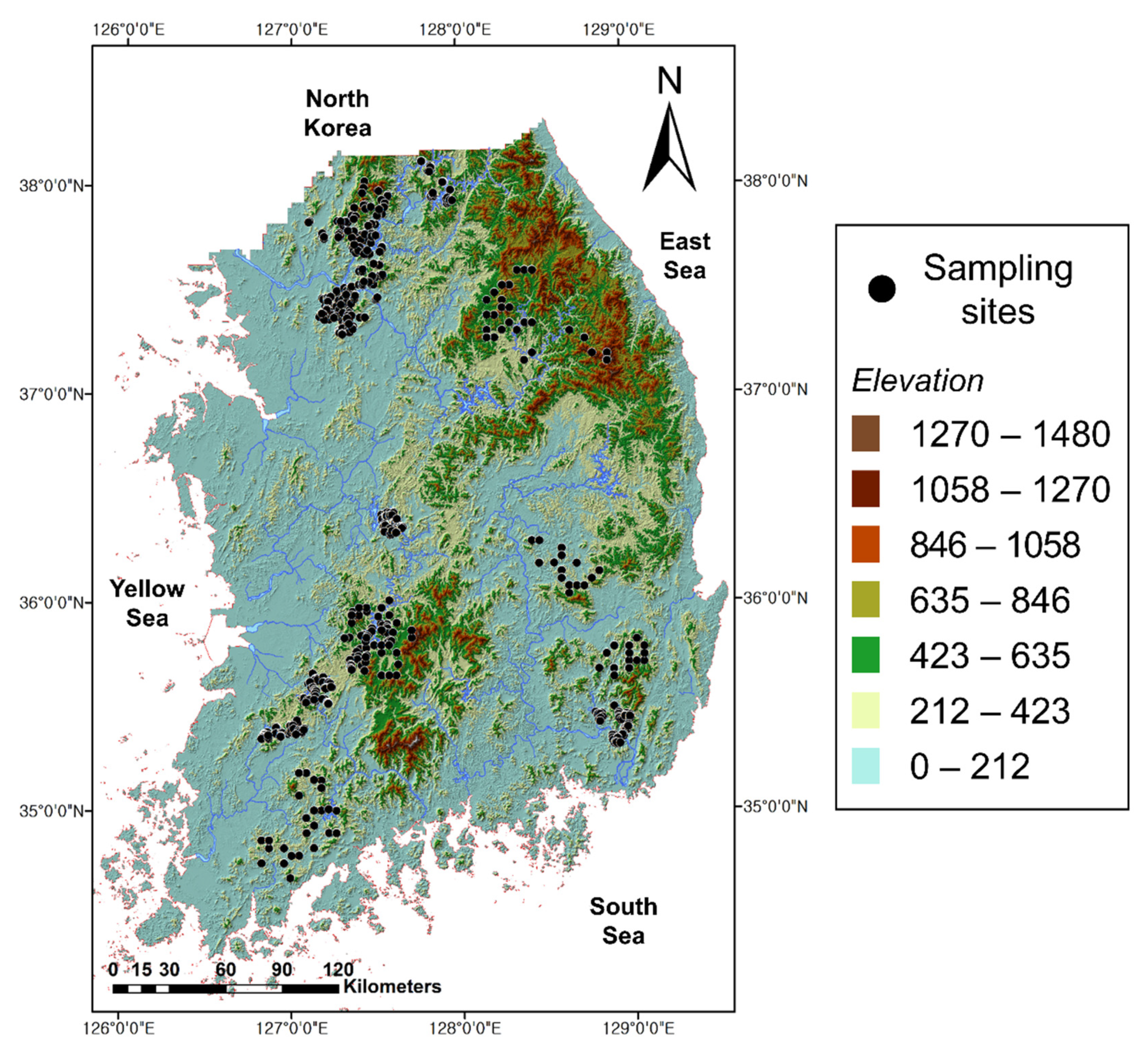
2.1. Study Sites

This study was conducted in South Korea, which is the southern half of the Korean Peninsula located in East Asia. The north side of South Korea is bordered by North Korea, and the other three sides are surrounded by the sea. It has a temperate climate and four seasons. The annual average temperature is about 12.8 degrees Celsius, and the annual average precipitation is about 1343 mm. After the Korean War ended in 1953, parts of the country were destroyed, and many trees were planted as a government policy. Now, almost two-thirds of South Korea, 62.8%, is covered by forests, in a context of complex topography.

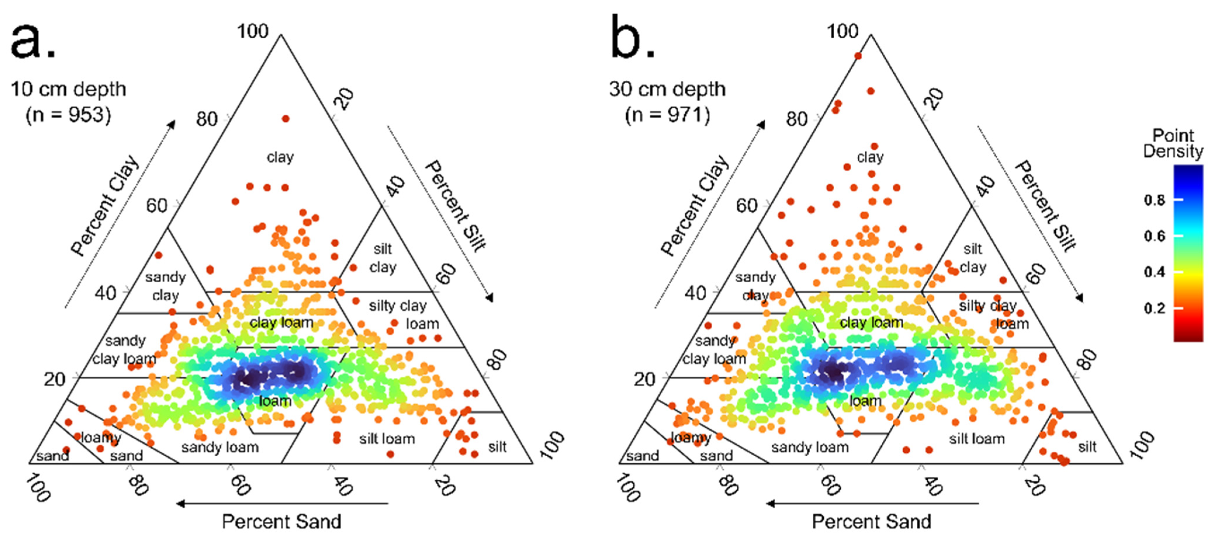
2.2. Forest Stand and Soil Properties

We used 11,544 soil samples collected at depths of 10 and 30 cm in a forested area of South Korea. These forest soil samples were collected by the National Institute of Forest Science to develop the SWHCs prediction models; soil samples were collected from 971 sample sites that were randomly selected (Figure 1). Nine hundred and seventy-one sample sites contain twelve soil texture classes, three forest types, and three kinds of bedrock (Figures S2 and S3). Six soil samples were collected in a sample site at the same point as replicates and collected at the equivalent soil depth (10 or 30 cm), though separated by a few centimeters. The soil texture distribution of the collected soil samples is shown in Figure 2.
All soil samples were collected below the organic O horizon. Since the average soil depth of A horizons in South Korean forests is about 17 to 20 cm, soil samples 10 cm deep represent mineral A horizons, while soil samples 30 cm deep represent B or C horizons.
In this study, three kinds of SWHCs are used: saturated water contents ( θ S ), water content at pF1.8 ( θ 1.8 ), and water content at pF2.7 ( θ 2.7 ). A pressure plate method was used to measure SWHCs. The collected soil samples were analyzed by means of laboratory methods to determine six physical and chemical properties, including bulk density and organic matter. Bulk density is related to soil compaction and structure. It was measured by the ratio of the dry weight of soil and the volume of the soil. Soil organic carbon was measured by the Walkley-Black method [20], and organic matter was recalculated by multiplying by 1.724, the van Bemmelen factor. Hydraulic conductivity was measured by the falling head method, which uses a constantly changing pressure head. Soil particle fractions were measured with the hydrometer method, and three particle-size classes were classified: sand (0.05 to 2 mm), silt (0.002 to 0.05 mm), and clay (<0.002 mm). In situ measurements were also investigated to develop PTFs for analysis of the environmental impact on soil. Dominant tree height, dominant tree DBH, average DBH, and tree density were measured by forestry professionals when soil samples were collected.
Soil type was not used as an explanatory variable in this study, because of its generality and diversity issues. The soil classification system for forest soil in South Korea is totally different from other classification systems such as World Reference Base for Soil Resources (WRB) or USDA soil taxonomy. In addition, because of the relatively small territory and the similar climatic zone throughout the whole country, over 86% of the forest soils are grouped in an order, Brown Forest Soils, which is similar to Inceptisols from USDA soil taxonomy. For example, about 87.4% of forest soils used in this study are Brown Forest Soils. Because of these reasons, soil type cannot be a useful variable for predicting SWHCs in South Korea, and we did not include the soil type as an input variable.
In Table 1, soil physical and chemical properties and forest stand characteristics are shown. Some soil samples at 10 cm depth from 18 sample sites were lost. Therefore, the number of analyzed soil sampling sites is different (n = 953 for 10 cm soil depth, n = 971 for 30 cm soil depth), and the averaged values of in situ measurements at 10 and 30 cm soil depth are different (Table 1).

2.3. Environmental Covariates

We extracted an environmental covariates dataset at corresponding soil sample sites from four geographical maps: digital elevation map (DEM; 10 m resolution), geologic map (GM; 1:50,000), forest type map (FTM; 1:25,000), and forest site and soil map (FSSM; 1:25,000). Eight topographic variables from the DEM, one bedrock variable from the GM, four forest stand characteristics from the FTM, and eight forest site and soil properties from the FSSM were selected to develop the DSM models (Table S1). We chose these 4 maps because they are open source and easily available at the National Geographic Information Institute. While all the variables in the PTF dataset were continuous, the environmental covariates dataset included 11 discrete variables (Table S1).

2.4. Random Forest Model

Random forest is one of the most popular machine learning methods. Unlike other machine learning models, the random forest model is appropriate for model development, as it has discrete input variables and is based on a decision tree algorithm. There are 11 discrete variables for developing DSM models, and this is the main reason why we used a random forest model to predict SWHCs in this study. The random forest model was established using Python (v. 3.7.4) and the RandomForestRegressor module from scikit-learn (v. 0.23.2).

2.5. Variable Importance Measurements

In this study, we selected two methods for calculating variable importance: feature importance and permutation importance. Feature importance is one of the most widely used methods for variable importance measurement in the random forest model. It is calculated based on mean decrease impurity. It is related to the random forest model structure and its developing process, where the decision tree is extended by impurity [21]. In other words, the greater the decrease in impurity, the higher the importance of the variable. We calculated the feature importance using scikit-learn version 0.23.2. Permutation importance is determined by the performance differences between a basic model and a modified model. The modified version uses an input variable in which one variable is randomly permutated and the others are fixed. If a critical variable is employed to develop the modified model, the performance of the new model will decrease more than that of a less important variable. In this paper, we used the coefficient of determination to measure the performance, with 500 times random analysis on each variable.

2.6. Linear Relationship

Pearson’s correlation coefficient is used to confirm the linear relationship between explanatory variables and SWHCs. It is a method used primarily in descriptive statistics, and it has a range from −1 to 1. As the absolute value of the correlation coefficient becomes larger, the linear relationship between the two variables becomes greater. A negative value means anti-correlation and a positive value means a positive relationship between two variables. The equation for Pearson’s correlation coefficient in this study is as follows:
r X Y = i = 1 N ( X i X ¯ ) ( Y i Y ¯ ) i = 1 N ( X i X ¯ ) 2 · i = 1 N ( Y i Y ¯ ) 2
where N is the sample size of variables X and Y.

2.7. Developed Models

A total of 12 random forest models were developed with different explanatory variables, soil sample layers, and matric suctions of response variables (Table 2). Explanatory variables are divided into two types: forest stand and soil physical and chemical properties for the PTF model and environmental covariates (Table S1) for the DSM model. We also classified soil sample layers at depths of 10 and 30 cm and soil water contents at saturated, pF1.8, and pF2.7 as the response variables.

2.8. Sensitivity Analysis

Sensitivity analysis can determine how much response variables are affected by explanatory variable changes. In this study, we conducted a sensitivity analysis using the developed random forest models. First, a soil sample was randomly chosen from the dataset. The explanatory variable became the input variable by changing equal intervals, while the others were kept constant. We used the modified variable as an input variable to test the sensitivity of the explanatory variable on the corresponding response variable. In this study, the analysis of each variable was repeated 150 times.
While scatter plotting and correlation coefficient analysis allow for an acknowledgement of the relationships between the explanatory variable and response variable, these analyses contain all the effects of variables that might affect response variable. On the other hand, sensitivity analysis enables the rejection of impacts of other variables on various models. Therefore, we can analyze the effects of one explanatory variable in greater detail.

3. Results

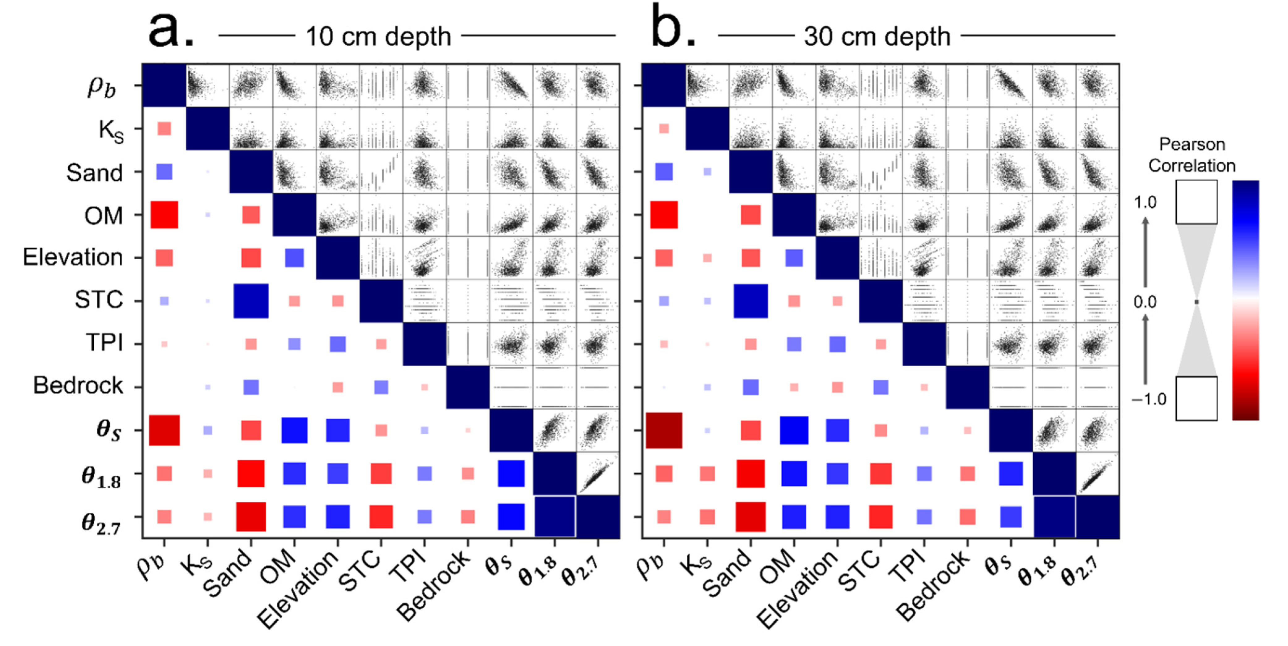
3.1. Variable Importance for Predicting SWHCs

Two methods were used for measuring variable importance. We standardized the variable importance of each model to have the total sum of 1. Feature importance and permutation importance were calculated by means of 12 models. Variable importance of forest stand, soil physical and chemical properties, and environmental covariates is shown in Tables S2–S4. To rank the importance of each variable, we averaged standardized feature importance and permutation importance (Figure 3). We also selected four critical variables for each model (Table 3).
As illustrated in Figure 3, variable importance to predict θ S , θ 1.8 , and θ 2.7 , respectively, has different characteristics. In the PTFs models that used forest stand and soil physical and chemical properties, bulk density greatly impacted on θ S prediction at both 10 and 30 cm. In predictions for θ 1.8 and θ 2.7 , however, the sand fraction was the most significant. Organic matter was critical for all cases, and hydraulic conductivity (KS) was also important. In the PTF-10-pF2.7 and PTF-30-pF2.7 models, the influence of clay increased, and the ranking of dominant tree height (DTH) on PTF-10-pF1.8 and PTF-30-pF2.7 went up, while the variable importance value remained low (below 6%).
In the DSM models that used environmental covariates as input variables, elevation was the primary important variable in θ S prediction at soil depths of 10 and 30 cm. To predict θ 1.8 and θ 2.7 , the soil texture class was the most significant. The next important variables were TPI and bedrock. In the DSM-10-pF0 model, aspect showed a high variable importance.
From the variable importance analysis, the importance difference by soil depth layer (10 and 30 cm) was not significant; however, the difference shown by different matric suctions was larger. The order of important variables between θ S and θ 1.8 showed a large difference, and the order of important difference between θ 1.8 and θ 2.7 was small, showing similar important variables (Table 3). The forest stand dataset influenced less than 11.6% in the PTF models (average 7.6%); therefore, soil physical and chemical properties were dominant in these models. In the DSM models, the digital elevation model (DEM) and forest site and soil maps (FSSM) showed more than 80% importance.

3.2. Correlation between Highly Effective Variables and SWHCs

From the variable importance analysis, we selected eight highly effective explanatory variables: four forest stand and soil physical and chemical properties ( ρ b , KS, sand, and OM) and four environmental covariates (elevation, STC, TPI, and bedrock). To identify the linear interrelationship between highly effective input variables and SWHCs, we plotted correlation matrix plots (Figure 4).
First, three kinds of SWHC were closely interrelated. The correlation coefficients of each relationship among the SWHCs were all positive, especially θ 1.8 and θ 2.7 . In soil physical and chemical properties, bulk density ( ρ b ) and sand fraction (sand) had a negative influence on SWHCs. Bulk density and organic matter showed a negative correlation with a high coefficient, and organic matter was positively related with SWHCs. All other variables except KS presented the same tendency to the three kinds of SWHCs. KS showed a positive correlation with θ S , but a negative correlation with θ 1.8 and θ 2.7 .
Regarding environmental covariate, elevation and TPI presented a positive relationship with SWHCs, and soil texture class and bedrock, which have a high correlation coefficient value to sand, showed a negative relationship with SWHCs. Elevation showed a high correlation with three soil properties. It had a negative relationship with bulk density and sand fraction and a positive relationship with organic matter. The differences in interrelationships between selected variables and SWHCs at soil depths of 10 cm and those at soil depths of 30 cm were not significant.

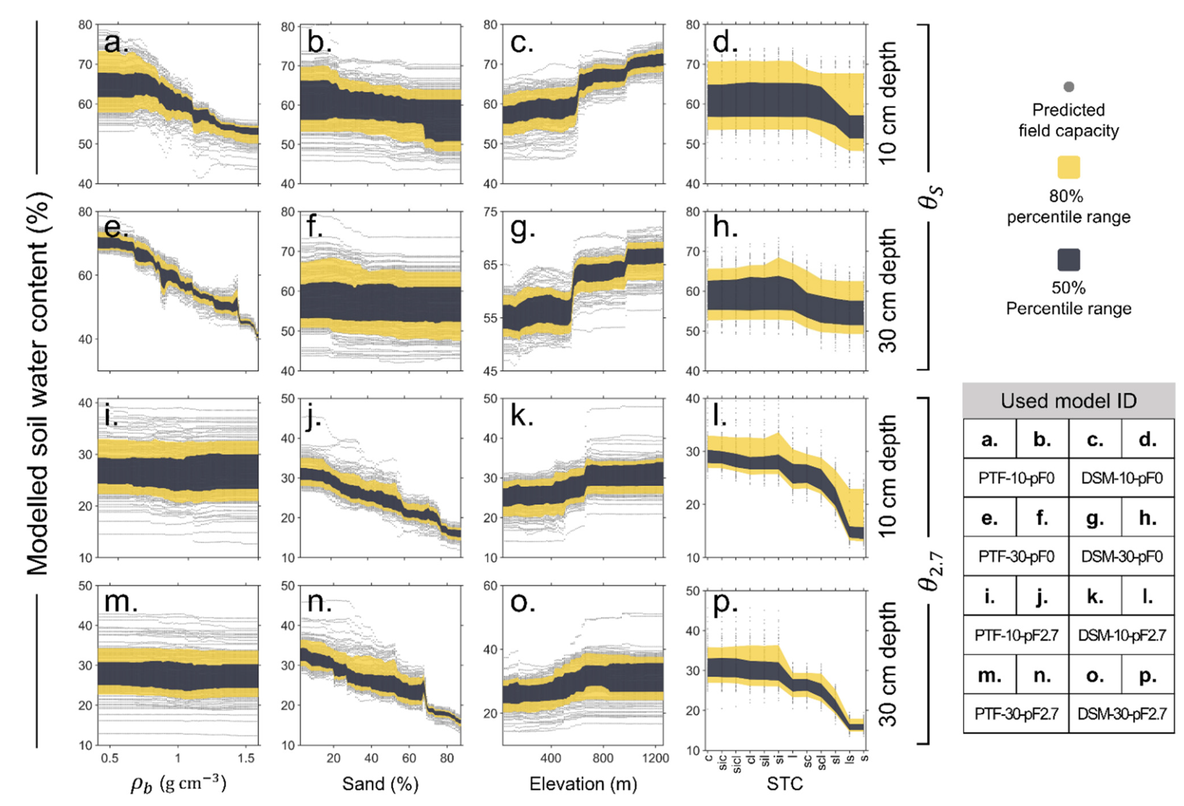
3.3. Sensitivity Analysis for Identifying Non-Linear Relationship

To identify the non-linear effect of input variables on SWHCs, a sensitivity analysis was conducted. We selected four variables that were primary and secondary important variables in PTF and DSM, respectively, and analyzed sensitivity on θ S and θ 2.7 (Figure 4). Since θ 1.8 and θ 2.7 are closely related (see in Figure 4) and have a similar trend, we excluded θ 1.8 from Figure 5.
In Figure 5a–h, θ S was highly sensitive to bulk density and elevation changes. As shown in Figure 4, bulk density has a negative relationship with θ S , and a positive relationship with elevation. Notably, θ S steeply increased at the elevation between 500 and 1000 m. On the other hand, sand fraction and soil texture classes showed a modest contribution when predicting θ S and presented a low sensitivity.
However, θ 2.7 showed the opposite tendency. Bulk density and elevation, which had high sensitivity in θ S , showed low sensitivity in θ 2.7 , and sand fraction and STC showed high sensitivity.
Figures S3–S6 depict sensitivity analysis results of the four selected variables from twelve developed models. From the sensitivity analysis, we confirmed the non-linear effects on SWHCs, not merely the linear relationship between two variables. For example, organic matter was significant only when it was below 5%. Hydraulic conductivity also showed a significant relationship only when KS < 0.02 cm s−1. Moreover, the impact of aspect on saturated soil water content was limited at a depth of 10 cm. The southern aspect (90 ° to 270 ° ) had a lower θ S than the northern aspect (0 ° to 90 ° and 270 ° to 360 ° ), the tendency of which was hardly detected by a linear relationship such as Pearson’s correlation.

4. Discussion

4.1. Influential Soil Physical and Chemical Properties on SWHCs Prediction

The primary important soil property to predict θ S was bulk density, while sand fraction was the most valuable in predicting θ 1.8 and θ 2.7 (Figure 3). Sensitivity analysis also demonstrated that the impact of bulk density and sand fraction on soil was different, along with different matric suction (Figures S3 and S4). Since bulk density is the mass of soil per unit volume, it represents soil structure and soil compaction [22]. The result of sensitivity analysis showed that an increase in the bulk density led to a decrease in θ S . Thus, compacted soil has fewer macropores and a lower water holding capacity.
On the other hand, sand fraction was the first important variable for predicting θ 1.8 and θ 2.7 , not silt or clay, which both showed a negative relationship. Since θ 2.7 is the amount of soil moisture after being pressured from pF1.8 and pF2.7 (−6.2 kPa and −49.1 kPa, respectively), soil water in macropore is eliminated at θ 2.7 [23]. Therefore, the trivial influence of bulk density on θ 1.8 and θ 2.7 prediction (below 4%) is explainable by soil texture, which is related to capillary force and micropore rather than macropore and soil structure.
The PTF-10-pF2.7 and PTF-30-pF2.7 models denoted that importance of the sand fraction became greater than that in predicting θ 1.8 , and it was also shown in sensitivity analysis results. Clay was significant in θ 2.7 prediction. Water holding capacity is closely related to capillary force [23]. As the particle of soil becomes finer, its surface area becomes broader; therefore, the capillary is enhanced. Soil needs a wider surface area and finer soil particles such as silt and clay to have more moisture at high matric suctions. In this regard, the enhanced role of the sand fraction in predicting θ 2.7 is indirect. The sand fraction is equal to the summation of the silt fraction and the clay fraction in hydrological modeling, since the sum of sand, silt, and clay is 100%. Small particles such as silt and clay become powerful in θ 1.8 and θ 2.7 predictions. Moreover, a higher rank of variable importance with a weight of 5~7% emphasizes the influence of clay in θ 2.7 , whereas the variable importance of the clay fraction for predicting θ S and θ 1.8 is minute (Figures S3 and S4).
In this vein, in order to estimate water holding capacity at a higher matric suction, such as θ 4.2 (water content at pF4.2; permanent wilting point), the importance of the clay fraction increases. Qiao et al. [24] employed a stepwise method to select proper variables for predicting θ 2.5 (field capacity) and θ 4.2 (permanent wilting point). While the sand fraction was used as the main factor in the θ 2.5 prediction, they selected clay as a main factor in the θ 4.2 prediction. Adhikary et al. [25] also used the clay fraction for θ 4.2 prediction, whereas the sand and silt fractions were used for θ 2.5 . As the capillary force is closely related to the soil texture (bulk density < sand < silt < clay), corresponding soil particle distribution mainly affects the SWHCs ( θ S < θ 1.8 < θ 2.7 < θ 4.2 ). In other words, soil structure is the main factor in θ S rather than soil texture, sand and silt are the major factors in θ 1.8 , and silt and clay are the most influential variables in θ 2.7 .
The relationship between the KS and SWHCs can be explained by the relation mentioned above. In Figure 4, KS has a positive correlation with θ S , but a negative correlation with θ 1.8 and θ 2.7 . KS and bulk density are negatively correlated, and compacted soil has smaller KS, since it has fewer macropores. On the other hand, the bulk density effect is negligible and soil texture is dominant in θ 1.8 and θ 2.7 . Therefore, a higher value of KS can be explainable through a high sand fraction content or a small clay fraction content, which are both closely related to the smaller value of θ 1.8 and θ 2.7 . The scatter plot in Figure 4 shows a weak correlation between KS and sand fraction; this is because KS is mainly affected by disturbances in the soil structure, indirectly caused by factors that affect bulk density and organic matter [22].
Organic matter was another powerful factor in the prediction of SWHCs. In Figures S3 and S4, SWHCs rise as organic matter contents become greater. The influence of organic matter on θ S is linked to bulk density. Organic matter enriches porosity and lessens soil compaction [26,27,28,29]. In particular, the negative relationship between organic matter and bulk density has been suggested as a linear equation in previous studies [30]. We also confirmed the linear relationship between bulk density and organic matter (BD = 1.26–0.073 OM; Figure 4). In other words, an increase in organic matter results in a reduction in bulk density and expansion of macropore; therefore, θ S rises.
Organic matter also affects water holding capacities. Many studies have confirmed that organic matter can increase θ 2.5 [3,31,32,33], which is closely related to θ 1.8 and θ 2.7 [5]. Leu et al. [32] confirmed that organic matter even increases in θ 4.2 . SWHCs are also highly related to the plant available water (PAW; generally represented as θ 2.5 - θ 4.2 or θ 1.8 - θ 2.7 ). Lal [34] demonstrated that the influence of organic matter on capillary force was more noticeable at field capacity ( θ 2.5 ) than at permanent wilting point ( θ 4.2 ), raising PAW. In this study, we also found similar results in our sensitivity analysis. In Figures S3 and S4, sensitivity on organic matter is higher at θ 1.8 than θ 2.7 . Thus, we identified that organic matter was effective in lower matric suction. We also confirmed that, when organic matter content is more than 5%, sensitivity dropped drastically. It is thought that organic matter with a large particle size is too large to affect capillary force. Consequently, soil organic matter shrinks bulk density and raises θ S and capillary force, as well as θ 1.8 and θ 2.7 . In this regard, we found that organic matter influenced SWHCs and PAW significantly. Its sensitivity was active below 5%, and it decreased sharply above 5%.

4.2. Interrelationship between Topography, Soil Properties, and Vegetation

Topography was also an influential factor in SWHCs. In previous studies, elevation, which was included in DEM, was the most dominant factor in predicting SWHCs [15,35,36]. In Figure 4, we confirm the interrelationships between elevation and soil physical and chemical properties. Elevation was closely related to bulk density, sand fraction, and organic matter of the soil. The sand fractions decreased and organic matter contents increased as the elevation became high. Most of Baekdudaegan, which is a mountain spine stretching from north to south in South Korea [37], is a nationally protected area. In this region, development is strictly limited, and natural vegetation is widely spread. It is considered that soil in high elevation has low bulk density and high organic matter contents because of these reasons. In addition, the effects of elevation on SWHCs can be found by the spatial distribution of bedrock. Since soil particles were made from bedrock, soil texture was highly related to its bedrock. Plaster et al. [38] showed the differences in soil textures from different bedrocks and sedimentary and metamorphic rocks. Metamorphic rock tends to create sand fraction, while sedimentary bedrock tends to create finer fractions. Soil samples in this study showed that the average elevation of sample sites with metamorphic rock was 286.7 m, and the average elevation of sample sites with sedimentary rock was 538.9 m. The average elevation of two types of bedrock is different and statistically significant (p < 0.01). This shows that finer fractions are more distributed in higher elevations due to the large distribution of sedimentary bedrock at high elevations.
In Figures S5 and S6, aspect was the most important topographical feature in the DSM-10-pF0 and DSM-30-pF0 models. Sensitivity analysis showed that the θ S of north-facing slopes was greater than the θ S of south-facing slopes. Solar energy in south-facing slopes, which is larger than that of north-facing slopes, raises soil and air temperatures of the mountainside. This could create water stress in plants and hinder the growth of vegetation, since high temperature increases evapotranspiration [39]. However, in South Korea, relatively high summer rainfall and annual rainfall, which is 1343 mm, generally limit water stress, and higher solar energy in south-facing slopes helps vegetation grow well. Vegetation and soil chemical weathering are highly related, and it can make soils in south-facing slopes finer [40,41,42]. Freeze–thaw processes could be another reason. In the winter season, the soil water freeze–thaw cycle is more frequent on south-facing slopes because of higher solar energy during the day; this cycle also promotes physical soil weathering [43,44], which could contribute to a greater relative abundance of finer particles and low θ S on south-facing slopes.

4.3. Limitations and Recommendations for Future Research

In this study, we collected data related to soil physical and chemical properties, environmental covariates, and forest stand characteristics to investigate the contribution factors of SWHCs. Forest stand characteristics data showed marginal effects on SWHC predictions compared to other variables, such as soil properties and topographical features [35]. It seems that the role of vegetation on soil moisture capacity is subtle; however, this is because we only used forest stand characteristics for biological factors. Understory vegetation plays a key role in affecting the moisture content of topsoil, organic matter content, and regional evapotranspiration [45]. In future research, the data of understory vegetation and NDVI, which represents overall vegetation, should be included to clarify the relationship among the soil physical and chemical properties, vegetation, and environmental covariates.
We used bulk density and soil texture for soil physical properties, and these variables showed great importance in predicting SWHCs. However, coarser soil particles over 2 mm were not considered for developing the models in this study. In future research, it may be more appropriate to include coarser soil particles to develop models and to confirm their interrelationships, since different size particles showed markedly different properties, as shown in Section 4.1.

5. Conclusions

The developed pedotransfer function (PTF) models based on forest stand and soil physical and chemical properties showed that bulk density had the greatest influence on predicting saturated water content ( θ S ), while sand content had the greatest influence on predicting water content at pF 1.8 and pF2.7 ( θ 1.8 and θ 2.7 ). The digital soil mapping (DSM) models developed using environmental covariates as an input dataset showed that elevation was the most influential factor in predicting θ S , and soil texture class was the most influential factor in predicting θ 1.8 and θ 2.7 .
Variable importance and sensitivity analysis showed that, as the matric suction changed, the soil physical and chemical properties that mainly influence the soil water holding capacities (SWHCs) changed to the following values: soil structure in θ S ; sand and silt fraction in θ 1.8 ; and much finer particles in θ 2.7 . It was confirmed that the organic material increased θ S by reducing the density and also increased θ 1.8 and θ 2.7 by increasing capillary force. The sensitivity of SWHCs to organic matter was significant when it was less than 5%. Elevation was closely related to the geological variability of bedrock and soil physical and chemical properties, and aspect was highly related to vegetation, confirming that it was an important variable for developing the DSM model.
This study contributes to the data collection process for the development of more accurate PTF and DSM models by presenting important variables necessary for the estimation of three kinds of SWHC. Unfortunately, we could not find a significant relationship between forest stand characteristics and SWHCs. However, we were able to confirm the close association with topographic features, soil physical and chemical properties, and vegetation. More accurate SWHCs prediction models will be developed when the data related to understory, NDVI data, and coarser soil particle are added.

Supplementary Materials

The following are available online at https://www.mdpi.com/article/10.3390/land10121290/s1. Table S1: Twenty-one environmental covariates from geographically referenced database used in this study; Table S2: Variable importance of forest stand and soil physical and chemical properties in PTF; Table S3: Variable importance of environmental covariates from digital elevation map and geologic map; Table S4: Variable importance of environmental covariates from forest type map and forest site and soil map; Figure S1: Spatial distribution of 971 soil sampling sites with soil texture map at 10 cm soil depth and 30 cm soil depth; Figure S2: Spatial distribution of 971 soil sampling sites with forest type map and geographical map; Figure S3: Modelled SWHCs changes across 4 important variables from sensitivity analysis and developed PTF models for soil depth at 10 cm; Figure S4: Modelled SWHCs changes across 4 important variables from sensitivity analysis and developed PTF models for soil depth at 30 cm; Figure S5: Modelled SWHCs changes across 4 important variables from sensitivity analysis and developed DSM models for soil depth at 10 cm; Figure S6: Modelled SWHC changes across 4 important variables from sensitivity analysis and developed DSM models for soil depth at 30 cm.

Author Contributions

Conceptualization, H.Y. (Hyunje Yang) and H.Y. (Hyeonju Yoo); methodology, H.Y. (Hyunje Yang) and H.Y. (Hyeonju Yoo); software, H.Y. (Hyunje Yang) and H.L.; validation, H.Y. (Hyunje Yang), H.Y. (Hyeonju Yoo) and H.T.C.; formal analysis, H.Y. (Hyunje Yang) and H.Y. (Hyeonju Yoo); investigation, H.Y. (Hyunje Yang), H.L., J.K. and H.T.C.; resources, H.Y. (Hyunje Yang), H.L., J.K. and H.T.C.; data curation, H.Y. (Hyunje Yang), H.L., J.K. and H.T.C.; writing—original draft preparation, H.Y. (Hyunje Yang) and H.Y. (Hyeonju Yoo); writing—review and editing, H.Y. (Hyunje Yang), H.Y. (Hyeonju Yoo), J.K. and H.T.C.; visualization, H.Y. (Hyunje Yang) and H.Y. (Hyeonju Yoo); supervision, H.Y. (Hyunje Yang), H.L. and H.T.C.; project administration, J.K. and H.T.C.; funding acquisition, J.K. and H.T.C. All authors have read and agreed to the published version of the manuscript.

Funding

This research received no external funding.

Data Availability Statement

Four geographically referenced maps used in this study (digital elevation map, geologic map, forest type map, and forest site and soil map) are available at the National Spatial Data Infrastructure Portal (http://www.nsdi.go.kr/lxportal/?menuno=2679 accessed on 4 October 2021) and National Geographic Information Institute (http://map.ngii.go.kr/mn/mainPage.do accessed on 4 October 2021). Additionally, in situ measurements used in this study are available from the corresponding author upon reasonable request.

Acknowledgments

We thank Yong Suk Kim for useful discussions. We also thank four anonymous referees for their invaluable comments on an earlier version of the manuscript.

Conflicts of Interest

The authors declare no conflict of interest.

References

  1. Götzinger, J.; Bárdossy, A. Comparison of four regionalisation methods for a distributed hydrological model. J. Hydrol. 2007, 333, 374–384. [Google Scholar] [CrossRef]
  2. Han, E.; Merwade, V.; Heathman, G.C. Implementation of Surface Soil Moisture Data Assimilation with Watershed Scale Distributed Hydrological Model. J. Hydrol. 2012, 416, 98–117. [Google Scholar] [CrossRef]
  3. Zhang, Y.; Cheng, G.; Li, X.; Han, X.; Wang, L.; Li, H.; Chang, X.; Flerchinger, G. Coupling of a simultaneous heat and water model with a distributed hydrological model and evaluation of the combined model in a cold region watershed. Hydrol. Process. 2013, 27, 3762–3776. [Google Scholar] [CrossRef]
  4. Vereecken, H.; Weynants, M.; Javaux, M.; Pachepsky, Y.; Schaap, M.G.; van Genuchten, M. Using Pedotransfer Functions to Estimate the van Genuchten-Mualem Soil Hydraulic Properties: A Review. Vadose Zone J. 2010, 9, 795–820. [Google Scholar] [CrossRef]
  5. Cianfrani, C.; Buri, A.; Vittoz, P.; Grand, S.; Zingg, B.; Verrecchia, E.; Guisan, A. Spatial modelling of soil water holding capacity improves models of plant distributions in mountain landscapes. Plant Soil 2019, 438, 57–70. [Google Scholar] [CrossRef] [Green Version]
  6. Kosugi, K. New diagrams to evaluate soil pore radius distribution and saturated hydraulic conductivity of forest soil. J. For. Res. 1997, 2, 95–101. [Google Scholar] [CrossRef]
  7. Hewelke, P.; Gnatowski, T.; Elp Tyszka, J.; Zakowicz, S. Analysis of Water Retention Capacity for Select Forest Soils in Poland. Pol. J. Environ. Stud. 2015, 24, 1013–1019. [Google Scholar] [CrossRef]
  8. Glp Duijnisveld, W.H.M.; Trinks, S. Hydro-Pedotransfer Functions (HPTFs) for Predicting Annual Percolation Rate on a Regional Scale. J. Hydrol. 2008, 356, 17–27. [Google Scholar]
  9. Zhang, Y.; Schaap, M.G.; Zha, Y. A High-Resolution Global Map of Soil Hydraulic Properties Produced by a Hierarchical Parameterization of a Physically Based Water Retention Model. Water Resour. Res. 2018, 54, 9774–9790. [Google Scholar] [CrossRef] [Green Version]
  10. Puckett, W.E.; Dane, J.H.; Hajek, B.F. Physical and Mineralogical Data to Determine Soil Hydraulic Properties. Soil Sci. Soc. Am. J. 1985, 49, 831–836. [Google Scholar] [CrossRef]
  11. Rawls, W.J.; Brakensiek, D. Estimating Soil Water Retention from Soil Properties. J. Irrig. Drain. Div. 1982, 108, 166–171. [Google Scholar] [CrossRef]
  12. Schaap, M.G.; Leij, F.J.; Van Genuchten, M.T. Neural Network Analysis for Hierarchical Prediction of Soil Hydraulic Properties. Soil Sci. Soc. Am. J. 1998, 62, 847–855. [Google Scholar] [CrossRef]
  13. Twarakavi, N.K.; Šimůnek, J.; Schaap, M.G. Development of Pedotransfer Functions for Estimation of Soil Hydraulic Parameters Using Support Vector Machines. Soil Sci. Soc. Am. J. 2009, 73, 1443–1452. [Google Scholar] [CrossRef] [Green Version]
  14. Ma, H.; Zeng, J.; Chen, N.; Zhang, X.; Cosh, M.H.; Wang, W. Satellite surface soil moisture from SMAP, SMOS, AMSR2 and ESA CCI: A comprehensive assessment using global ground-based observations. Remote. Sens. Environ. 2019, 231, 111215. [Google Scholar] [CrossRef]
  15. Fathololoumi, S.; Vaezi, A.R.; Alavipanah, S.K.; Ghorbani, A.; Saurette, D.; Biswas, A. Effect of Multi-Temporal Satellite Images on Soil Moisture Prediction Using a Digital Soil Mapping Approach. Geoderma 2021, 385, 114901. [Google Scholar] [CrossRef]
  16. Gooley, L.; Huang, J.; Page, D.; Triantafilis, J. Digital soil mapping of available water content using proximal and remotely sensed data. Soil Use Manag. 2014, 30, 139–151. [Google Scholar] [CrossRef]
  17. Jeihouni, M.; Alavipanah, S.K.; Toomanian, A.; Jafarzadeh, A.A. Digital mapping of soil moisture retention properties using solely satellite-based data and data mining techniques. J. Hydrol. 2020, 585, 124786. [Google Scholar] [CrossRef]
  18. Akpa, S.I.C.; Odeh, I.O.A.; Bishop, T.; Hartemink, A. Digital Mapping of Soil Particle-Size Fractions for Nigeria. Soil Sci. Soc. Am. J. 2014, 78, 1953–1966. [Google Scholar] [CrossRef] [Green Version]
  19. Mahmoudabadi, E.; Karimi, A.; Haghnia, G.H.; Sepehr, A. Digital soil mapping using remote sensing indices, terrain attributes, and vegetation features in the rangelands of northeastern Iran. Environ. Monit. Assess. 2017, 189, 500. [Google Scholar] [CrossRef]
  20. Walkley, A.; Black, I.A. An examination of the Degtjareff method for determining soil organic matter, and a proposed modification of the chromic acid titration method. Soil Sci. 1934, 37, 29–38. [Google Scholar] [CrossRef]
  21. Breiman, L.; Friedman, J.H.; Olshen, R.A.; Stone, C.J. Classification and Regression Trees; Routledge: Boca Raton, FL, USA, 1984; p. 368. [Google Scholar]
  22. Araya, S.N.; Ghezzehei, T.A. Using Machine Learning for Prediction of Saturated Hydraulic Conductivity and Its Sensitivity to Soil Structural Perturbations. Water Resour. Res. 2019, 55, 5715–5737. [Google Scholar] [CrossRef]
  23. Latshaw, K.; Fitzgerald, J.; Sutton, R. Analysis of Green Roof Growing Media Porosity. RURALS 2009, 4, 2. [Google Scholar]
  24. Qiao, J.; Zhu, Y.; Jia, X.; Huang, L.; Shao, M. Pedotransfer functions for estimating the field capacity and permanent wilting point in the critical zone of the Loess Plateau, China. J. Soils Sediments 2019, 19, 140–147. [Google Scholar] [CrossRef]
  25. Adhikary, P.P.; Chakraborty, D.; Kalra, N.; Sachdev, C.B.; Patra, A.K.; Kumar, S.; Tomar, R.K.; Chandna, P.; Raghav, D.; Agrawal, K.; et al. Pedotransfer functions for predicting the hydraulic properties of Indian soils. Soil Res. 2008, 46, 476–484. [Google Scholar] [CrossRef]
  26. Ekwue, E.; Stone, R. Effect of Peat on the Compactibility of Some Trinidadian Soils. J. Agric. Eng. Res. 1994, 57, 129–136. [Google Scholar] [CrossRef]
  27. Li, X.-G.; Li, F.-M.; Zed, R.; Zhan, Z.-Y.; Singh, B. Soil physical properties and their relations to organic carbon pools as affected by land use in an alpine pastureland. Geoderma 2007, 139, 98–105. [Google Scholar] [CrossRef]
  28. Ohu, J.O.; Raghavan, G.S.V.; McKyes, E. Peatmoss Effect on the Physical and Hydraulic Characteristics of Compacted Soils. Trans. ASAE 1985, 28, 420–424. [Google Scholar] [CrossRef]
  29. Wagner, L.E.; Ambe, N.M.; Ding, D. Estimating a Proctor Density Curve from Intrinsic Soil Properties. Trans. ASAE 1994, 37, 1121–1125. [Google Scholar] [CrossRef]
  30. Zhang, H.; Hartge, K.H.; Ringe, H. Effectiveness of Organic Matter Incorporation in Reducing Soil Compactibility. Soil Sci. Soc. Am. J. 1997, 61, 239–245. [Google Scholar] [CrossRef]
  31. Gardner, W.; Broersma, K.; Naeth, M.A.; Chanasyk, D.; Jobson, A. Influence of biosolids and fertilizer amendments on physical, chemical and microbiological properties of copper mine tailings. Can. J. Soil Sci. 2010, 90, 571–583. [Google Scholar] [CrossRef]
  32. Leu, J.M.; Traore, S.; Wang, Y.M.; Kan, C.E. The Effect of Organic Matter Amendment on Soil Water Holding Capacity Change for Irrigation Water Saving: Case Study in Sahelian Environment of Africa. Sci. Res. Essays 2010, 5, 3564–3571. [Google Scholar]
  33. Rawls, W.; Pachepsky, Y.; Ritchie, J.; Sobecki, T.; Bloodworth, H. Effect of soil organic carbon on soil water retention. Geoderma 2003, 116, 61–76. [Google Scholar] [CrossRef]
  34. Lal, R. Soil organic matter and water retention. Agron. J. 2020, 112, 3265–3277. [Google Scholar] [CrossRef]
  35. Jin, X.; Wang, S.; Yu, N.; Zou, H.; An, J.; Zhang, Y.; Wang, J. Spatial predictions of the permanent wilting point in arid and semi-arid regions of Northeast China. J. Hydrol. 2018, 564, 367–375. [Google Scholar] [CrossRef]
  36. Obi, J.; Ogban, P.; Ituen, U.; Udoh, B. Development of Pedotransfer Functions for Coastal Plain Soils Using Terrain Attributes. Catena 2014, 123, 252–262. [Google Scholar] [CrossRef]
  37. Lim, H.; Yang, H.; Chun, K.W.; Choi, H.T. Development of Pedo-Transfer Functions for the Saturated Hydraulic Conductivity of Forest Soil in South Korea Considering Forest Stand and Site Characteristics. Water 2020, 12, 2217. [Google Scholar] [CrossRef]
  38. Plaster, R.W.; Sherwood, W.C. Bedrock Weathering and Residual Soil Formation in Central Virginia. GSA Bull. 1971, 82, 2813–2826. [Google Scholar] [CrossRef]
  39. Hanna, A.Y.; Harlan, P.W.; Lewis, D.T. Soil Available Water as Influenced by Landscape Position and Aspect 1. Agron. J. 1982, 74, 999–1004. [Google Scholar] [CrossRef]
  40. Molina, A.; Vanacker, V.; Corre, M.D.; Veldkamp, E. Patterns in Soil Chemical Weathering Related to Topographic Gradients and Vegetation Structure in a High Andean Tropical Ecosystem. J. Geophys. Res. Earth Surf. 2019, 124, 666–685. [Google Scholar] [CrossRef]
  41. Rech, J.A.; Reeves, R.W.; Hendricks, D.M. The influence of slope aspect on soil weathering processes in the Springerville volcanic field, Arizona. Catena 2001, 43, 49–62. [Google Scholar] [CrossRef]
  42. Walker, J.; Thompson, C.H.; Jehne, W. Soil Weathering Stage, Vegetation Succession, and Canopy Dieback. Pac. Sci. 1983, 37, 471–481. [Google Scholar]
  43. Deprez, M.; De Kock, T.; De Schutter, G.; Cnudde, V. A review on freeze-thaw action and weathering of rocks. Earth-Sci. Rev. 2020, 203, 103143. [Google Scholar] [CrossRef]
  44. Matsuoka, N.; Murton, J. Frost weathering: Recent advances and future directions. Permafr. Periglac. Process. 2008, 19, 195–210. [Google Scholar] [CrossRef]
  45. Cierjacks, A.; Kleinschmit, B.; Kowarik, I.; Graf, M.; Lang, F. Organic matter distribution in floodplains can be predicted using spatial and vegetation structure data. River Res. Appl. 2011, 27, 1048–1057. [Google Scholar] [CrossRef]
Figure 1. Spatial distribution of 971 soil sampling sites in South Korea.
Land 10 01290 g001
Figure 2. Soil texture distribution used in this study: (a) distribution of soil samples at 10 cm depth and (b) 30 cm depth. Twelve soil textures (<2 mm fraction) were determined according to USDA Textural Soil Classification.
Land 10 01290 g002
Figure 3. Averaged variable importance of 30 explanatory variables.
Land 10 01290 g003
Figure 4. Correlation matrix of 8 highly important variables and SWHCs.
Land 10 01290 g004
Figure 5. Non-linear changes in modelled soil water content by sensitivity analysis. Modelled soil water content changes of (ad) θ S at 10 cm depth soil, (eh) θ S at 30 cm depth soil, (il) θ 2.7 at 10 cm depth soil, (mp) θ 2.7 at 30 cm depth soil were represented with four variables: bulk density, sand fraction, elevation, and soil texture class.
Land 10 01290 g005
Table 1. Measured forest stand and soil physical and chemical properties.
Forest Stand and Soil Physical and Chemical PropertiesAbb.UnitAt 10 cm Soil Depth (n = 953)At 30 cm Soil Depth (n = 971)
Saturated SWC θ S % 60.4   ±   7.9 57.7   ±   7.5
SWC at pF1.8 θ 1.8 % 32.2   ±   6.8 33.0   ±   7.2
SWC at pF2.7 θ 2.7 % 26.3   ±   5.8 27.4   ±   6.5
Bulk density ρ b g cm−3 0.95   ±   0.2 1.05   ±   0.2
Organic matterOM% 4.07   ±   1.88 2.98   ±   1.52
Hydraulic conductivity K S cm s−1 0.015   ±   0.013 0.011   ±   0.010
Sand fractionSand% 39.5   ±   16.3 38.4   ±   17.2
Silt fractionSilt% 37.6   ±   15.7 36.2   ±   16.7
Clay fractionClay% 22.8   ±   10.3 25.4   ±   11.8
Dominant tree heightDTHm 14.7   ±   3.5 14.6   ±   3.4
Dominant tree DBHDTDcm 30.6   ±   10.2 30.4   ±   9.9
Average DBHADcm 24.0   ±   7.5 23.7   ±   7.4
Tree densityTDtrees ha−1 578   ±   285 580   ±   283
Note: Average   ±   standard deviation. DBH is diameter at breast height.
Table 2. Developed models.
Model IDExplanatory VariablesSoil Sample LayerMatric Suction of Response Variable
PTF-10-pF0Forest stand and soil physical and chemical properties10 cm depthpF0 (saturated)
PTF-10-pF1.8pF1.8
PTF-10-pF2.7pF2.7
PTF-30-pF030 cm depthpF0 (saturated)
PTF-30-pF1.8pF1.8
PTF-30-pF2.7pF2.7
DSM-10-pF0Environmental covariates10 cm depthpF0 (saturated)
DSM-10-pF1.8pF1.8
DSM-10-pF2.7pF2.7
DSM-30-pF030 cm depthpF0 (saturated)
DSM-30-pF1.8pF1.8
DSM-30-pF2.7pF2.7
Table 3. Four primary important variables of the twelve developed models.
Model IDFirst
Important Variable
Second
Important Variable
Third
Important Variable
Fourth
Important Variable
PTF-10-pF0 ρ b OMSand K S
PTF-10-pF1.8SandOM K S DTH
PTF-10-pF2.7SandOM K S Clay
PTF-30-pF0 ρ b OMSandClay
PTF-30-pF1.8Sand K S OMDTH
PTF-30-pF2.7Sand K S OMClay
DSM-10-pF0ElevationAspectSTCTSD
DSM-10-pF1.8STCElevationTPIBedrock
DSM-10-pF2.7STCElevationTPIAspect
DSM-30-pF0ElevationSTCAspectTPI
DSM-30-pF1.8STCElevationTPIBedrock
DSM-30-pF2.7STCElevationBedrockTPI
Publisher’s Note: MDPI stays neutral with regard to jurisdictional claims in published maps and institutional affiliations.

