
Exploring the Effects of Contextual Factors on Residential Land Prices Using an Extended Geographically and Temporally Weighted Regression Model

Abstract
:1. Introduction
2. Materials and Methods
2.1. Study Area
2.2. Data Source
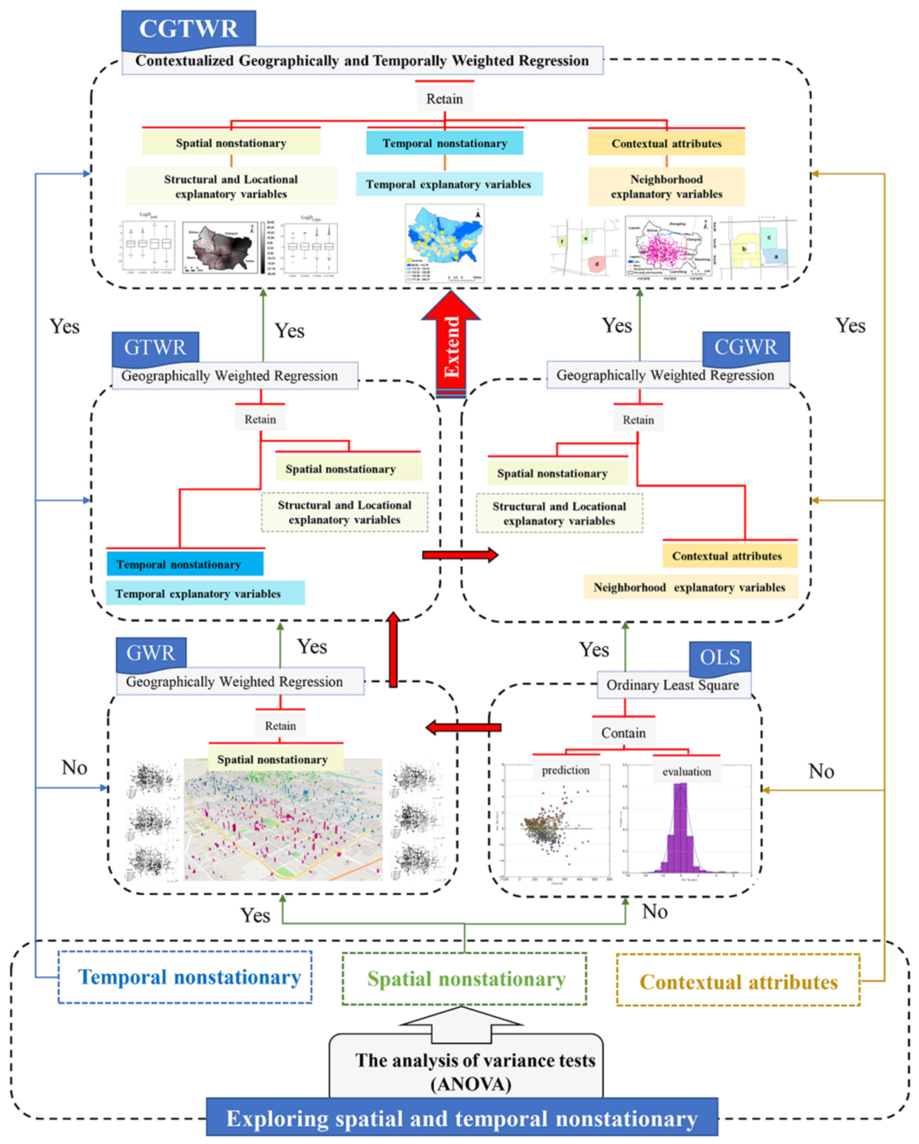
2.3. Methods
2.3.1. Geographically and Temporally Weighted Regression
2.3.2. Extension to GTWR with Neighborhood-Level Similarity
| Algorithm 1. Pseudo-code describing the CGTWR model. |
| Algorithm: CGTWR |
| INPUT: explanatory variables X spatiotemporal coordinates dependent variable Y |
| PROCESS: |
| Find the optimal spatial bandwidth , golden section search G1: |
| for do |
| construct the spatial kernel weight between and |
| calculate the CV value |
| end for |
| Achieve the optimal spatial bandwidth |
| Find the optimal spatiotemporal factor , implement golden section search G2 |
| Find the optimal contextual factor , implement golden section search G3 |
| for do |
| construct the contextual spatiotemporal kernel weight between and |
| calculate the CV value |
| end for |
| Find the optimal contextual factor and spatiotemporal factor |
| Calculate RSS, MSE, AIC, |
2.3.3. Model Evaluation of Performance
3. Experimental Results and Comparisons
3.1. Results of the Global Model
3.2. Results of the Local Model
4. Discussion and Policy Implications
4.1. The Performance of the Model in Exploring Spatiotemporal Heterogeneity
4.2. The Impact Factors of Policy Driven by Residential Land Prices
5. Conclusions
Author Contributions
Funding
Institutional Review Board Statement
Informed Consent Statement
Data Availability Statement
Conflicts of Interest
References
- Dunsky, R.M.; Follain, J.R.; Giertz, S.H. Pricing Credit Risk for Mortgages: Credit Risk Spreads and Heterogeneity across Housing Markets. Real Estate Econ. 2021, 21, 997–1032. [Google Scholar] [CrossRef]
- Stockhammer, E.; Bengtsson, E. Financial effects in historic consumption and investment functions. Int. Rev. Appl. Econ. 2020, 34, 304–326. [Google Scholar] [CrossRef] [Green Version]
- Qu, Y.B.; Jiang, G.H.; Li, Z.T.; Shang, R.; Zhou, D.Y. Understanding the multidimensional morphological characteristics of urban idle land: Stage, subject, and spatial heterogeneity. Cities 2020, 97, 102492. [Google Scholar] [CrossRef]
- Cabras, I.; Sohns, F.; Canduela, J.; Toms, S. Public houses and house prices in Great Britain: A panel analysis. Eur. Plan. Stud. 2020, 29, 163–180. [Google Scholar] [CrossRef] [Green Version]
- Solar, P.M. China’s GDP: Some Corrections and the Way Forward. J. Econ. Hist. 2021, 81, 943–957. [Google Scholar] [CrossRef]
- Gong, P.; Liang, S.; Carlton, E.J.; Jiang, Q.W.; Wu, J.Y.; Wang, L.; Remais, J.V. Urbanisation and health in China. Lancet 2012, 379, 843–852. [Google Scholar] [CrossRef]
- Harten, J.G.; Kim, A.M.; Brazier, J.C. Real and fake data in Shanghai’s informal rental housing market: Ground truthing data scraped from the internet. Urban Stud. 2021, 58, 1831–1845. [Google Scholar] [CrossRef]
- Schneider, A.; Woodcock, C.E. Compact, Dispersed, Fragmented, Extensive? A Comparison of Urban Growth in Twenty-five Global Cities using Remotely Sensed Data, Pattern Metrics and Census Information. Urban Stud. 2014, 45, 659–692. [Google Scholar] [CrossRef]
- Alm, J.; Lai, W.Z.; Li, X. Housing market regulations and strategic divorce propensity in China. J. Popul. Econ. 2021, 25, 1–29. [Google Scholar]
- Hussain, T.; Abbas, J.; Wei, Z.; Ahmad, S.; Bai, X.H. Impact of Urban Village Disamenity on Neighboring Residential Properties: Empirical Evidence from Nanjing through Hedonic Pricing Model Appraisal. Urban Plan. Dev. 2020, 147, 04020055. [Google Scholar] [CrossRef]
- Seo, B.K.; Park, G.R. Food insecurity and housing affordability among low-income families: Does housing assistance reduce food insecurity? Public Health Nutr. 2021, 24, 4339–4345. [Google Scholar] [CrossRef]
- Gao, Y.Y.; Zang, L.Z.; Sun, J. Does Computer Penetration Increase Farmers’ Income? An Empirical Study from China. Telecommun. Policy 2018, 42, 345–360. [Google Scholar] [CrossRef]
- Cheung, K.S.; Wong, S.K. Entry and Exit Affordability of Shared Equity Homeownership: An International Comparison. Soc. Sci. Electron. Publ. 2020, 13, 737–752. [Google Scholar] [CrossRef]
- Wallner, R. GIS measures of residential property views. J. Real Estate Lit. 2014, 20, 224–225. [Google Scholar] [CrossRef]
- Sesli, F.A. Creating real estate maps by using GIS: A case study of Atakum Samsun/Turkey. Acta Montan. Slovaca 2015, 20, 260–270. [Google Scholar]
- Morano, P.; Tajani, F.; Locurcio, M. GIS application and econometric analysis for the verification of the financial feasibility of roof-top wind turbines in the city of Bari (Italy). Renew. Sustain. Energy Rev. 2017, 70, 999–1010. [Google Scholar] [CrossRef]
- Chmielewska, A.; Adamiczka, J.; Romanowski, M. Genetic Algorithm as Automated Valuation Model Component in Real Estate Investment Decisions System. Real Estate Manag. Valuat. 2020, 28, 1–14. [Google Scholar] [CrossRef]
- Jacquet-Lagreze, E.; Siskos, J. Assessing a set of additive utility functions for multicriteria decision-making, the UTA method. Eur. J. Oper. Res. 1982, 10, 151–164. [Google Scholar] [CrossRef]
- Morano, P.; Tajani, F.; Locurcio, M. Multicriteria analysis and genetic algorithms for mass appraisals in the Italian property market. Int. J. Hous. Mark. Anal. 2018, 11, 229–262. [Google Scholar] [CrossRef]
- Guarini, M.R.; Locurcio, M.; Battisti, F. GIS-Based Multi-criteria Decision Analysis for the “Highway in the Sky”. International Conference on Computational Science and Its Applications. Springer Int. Publ. 2015, 9157, 146–161. [Google Scholar]
- Dong, S.H.; Wang, Y.D.; Gu, Y.Y.; Shao, S.W.; Liu, H.; Wu, S.M.; Li, M.M. Predicting the turning points of housing prices by combining the financial model with genetic algorithm. PLoS ONE 2020, 15, 457–461. [Google Scholar] [CrossRef]
- Ahn, J.J.; Byun, H.W.; Oh, K.J.; Kim, T.Y. Using ridge regression with genetic algorithm to enhance real estate appraisal forecasting. Expert Syst. Appl. 2012, 39, 8369–8379. [Google Scholar] [CrossRef]
- Brunsdon, C.; Fotheringham, A.S.; Charlton, M.E. Geographically Weighted Regression: A Method for Exploring Spatial Nonstationarity. Geogr. Anal. 1996, 28, 281–298. [Google Scholar] [CrossRef]
- Brunsdon, C.; Fotheringham, A.S.; Charlton, M.E. Spatial Nonstationarity and Autoregressive Models. Environ. Plan. A 1998, 30, 957–973. [Google Scholar] [CrossRef]
- Harris, P.; Fotheringham, A.S.; Crespo, R. The Use of Geographically Weighted Regression for Spatial Prediction: An Evaluation of Models Using Simulated Data Sets. Math. Geosci. 2010, 42, 657–680. [Google Scholar] [CrossRef]
- Brunsdon, C.; Fotheringham, A.S.; Charlton, M.E. Some Notes on Parametric Significance Test for Geographically Weighted Regression. J. Reg. Sci. 1999, 39, 497–524. [Google Scholar] [CrossRef]
- Habib, M.; Miller, E. Influence of Transportation Access and Market Dynamics on Property Values: Multilevel Spatiotemporal Models of Housing Price. Transp. Res. Rec. J. Transp. Res. Board 2008, 2076, 183–191. [Google Scholar] [CrossRef]
- Huang, B.; Wu, B.; Barry, M. Geographically and temporally weighted regression for modeling Spatio-temporal variation in house prices. Int. J. Geogr. Inf. Sci. 2010, 24, 383–401. [Google Scholar] [CrossRef]
- Fotheringham, A.S.; Kelly, M.H.; Charlton, M. The demographic impacts of the Irish famine: Towards a greater geographical understanding. Trans. Inst. Br. Geogr. 2013, 38, 221–237. [Google Scholar] [CrossRef]
- Harris, R.; Dong, G.; Zhang, W. Using contextualized Geographically Weighted Regression to model the spatial heterogeneity of land prices in Beijing, China. Trans. GIS 2013, 17, 901–919. [Google Scholar] [CrossRef]
- Beracha, E.; Gilbert, B.T.; Kjorstad, T. On the Relation between Local Amenities and House Price Dynamics. Real Estate Econ. 2018, 46, 612–654. [Google Scholar] [CrossRef]
- Abidoye, R.B.; Chan, A.P.C. Improving property valuation accuracy: A comparison of hedonic pricing model and artificial neural network. Pac. Rim Prop. Res. J. 2018, 24, 71–83. [Google Scholar] [CrossRef]
- Weir, R. Using geographically weighted regression to explore neighborhood-level predictors of domestic abuse in the UK. Trans. GIS 2019, 23, 1232–1250. [Google Scholar] [CrossRef]
- Baborska-Narozny, M.; Stevenson, F.; Chatterton, P. Temperature in housing: Stratification and contextual factors. Proc. Inst. Civ. Eng. Eng. Sustain. 2015, 169, 125–137. [Google Scholar] [CrossRef] [Green Version]
- Weimer, D.L.; Wolkoff, M.J. School Performance and Housing Values: Using Non-Contiguous District and Incorporation Boundaries to Identify School Effects. Natl. Tax J. 2001, 54, 231–253. [Google Scholar] [CrossRef] [Green Version]
- Bates, L.K. Does Neighborhood really matter? Comparing historically defined neighborhood boundaries with housing submarkets. J. Plan. Educ. Res. 2006, 26, 5–17. [Google Scholar] [CrossRef]
- Fontes, T.; Li, P.L.; Barros, N.; Zhao, P.J. Trends of PM2.5 concentrations in China: A long term approach. J. Environ. Manag. 2017, 196, 719–732. [Google Scholar] [CrossRef] [PubMed]
- Majeed, H. Consideration of local geographical variations in PM2.5 concentrations in China. Lancet Public Health 2014, 3, 564. [Google Scholar] [CrossRef] [Green Version]
- Kim, Y.; Kim, J.Y.; Lee, S.B.; Moon, K.C.; Bae, G.N. Review on the Recent PM2.5 Studies in China. J. Korean Soc. Atmos. Environ. 2015, 31, 411–429. [Google Scholar] [CrossRef] [Green Version]
- Apte, J.S.; Marshall, J.D.; Cohen, A.J.; Brauer, M. Addressing Global Mortality from Ambient PM2.5. Environ. Sci. Technol. 2015, 49, 8057–8066. [Google Scholar] [CrossRef]
- Gao, A.F.; Wang, J.Y.; Luo, J.F.; Li, A.G.; Chen, K.Y.; Wang, P.F.; Wang, Y.Y.; Li, J.Y.; Hu, J.L.; Zhang, H.L. Temporal variation of PM 2.5-associated health effects in Shijiazhuang, Hebei. Front. Environ. Sci. Eng. 2021, 15, 82. [Google Scholar] [CrossRef]
- Rosen, S. Hedonic prices and implicit markets: Product differentiation in pure competition. J. Political Econ. 1974, 82, 34–55. [Google Scholar] [CrossRef]
- Mian, A.; Sufi, A. House Prices, Home Equity-Based Borrowing, and the U.S. Household Leverage Crisis. Am. Econ. Rev. 2009, 101, 2132–2156. [Google Scholar] [CrossRef] [Green Version]
- Lisi, G. Hedonic pricing models and residual house price volatility. Lett. Spat. Resour. Sci. 2019, 12, 133–142. [Google Scholar] [CrossRef]
- Liu, J.; Yang, Y.; Xu, S.; Zhao, Y.; Wang, Y.; Zhang, F. A Geographically Temporal Weighted Regression Approach with Travel Distance for House Price Estimation. Entropy 2016, 18, 303. [Google Scholar] [CrossRef]
- Cossu, L.; Zanardo, P.; Zannier, U. Products of elementary matrices and non-Euclidean principal ideal domains. J. Algebra 2018, 501, 182–205. [Google Scholar] [CrossRef]
- Anderson, M.J. Distance-Based Tests for Homogeneity of Multivariate Dispersions. Biometrics 2006, 62, 245–253. [Google Scholar] [CrossRef] [PubMed]
- Abbas, K.; Liu, M.; Venkatesh, M.; Amico, E.; Kaplan, A.D.; Ventresca, M.; Pessoa, L.; Harezlak, J.; Goñi, J. Geodesic distance on optimally regularized functional connectomes uncovers individual fingerprints. Brain Connect. 2021, 11, 333–348. [Google Scholar] [CrossRef] [PubMed]
- Disatnik, D.; Sivan, L. The multicollinearity illusion in moderated regression analysis. Mark. Lett. 2016, 27, 403–408. [Google Scholar] [CrossRef]
- Hong, Z.; Mei, C.; Wang, H.; Du, W. Spatiotemporal effects of climate factors on childhood hand, foot, and mouth disease: A case study using mixed geographically and temporally weighted regression models. Int. J. Geogr. Inf. Sci. 2021, 35, 1611–1633. [Google Scholar] [CrossRef]
- Guo, B.; Wang, X.; Pei, L.; Su, Y.; Zhang, D.; Wang, Y. Identifying the spatiotemporal dynamic of PM2.5 concentrations at multiple scales using geographically and temporally weighted regression model across China during 2015–2018. Sci. Total Environ. 2020, 751, 141765. [Google Scholar] [CrossRef]
- Fotheringham, A.S.; Crespo, R.; Yao, J. Geographical and Temporal Weighted Regression (GTWR). Geogr. Anal. 2015, 47, 431–452. [Google Scholar] [CrossRef] [Green Version]
- Meagan, C.; Gordon, M. Using Geographically Weighted Regression to Explore Local Crime Patterns. Soc. Sci. Comput. Rev. 2007, 25, 174–193. [Google Scholar]
- McMillen, D.P. Geographically Weighted Regression: The Analysis of Spatially Varying Relationships. Am. J. Agric. Econ. 2004, 86, 554–556. [Google Scholar] [CrossRef]
- Hudson, C. Governing the governance of education: The state strikes back? Eur. Educ. Res. J. 2007, 6, 266–282. [Google Scholar] [CrossRef] [Green Version]
- Portz, J. “Next-Generation” Accountability? Evidence From Three School Districts. Urban Educ. 2017, 56, 1297–1327. [Google Scholar] [CrossRef]
- Clapp, J.M.; Nanda, A.; Ross, S.L. Which school attributes matter? The influence of school district performance and demographic composition on property values. J. Urban Econ. 2008, 63, 451–466. [Google Scholar] [CrossRef] [Green Version]
- Hooge, E.H.; Moolenaar, N.M.; Look, K.; Janssen, S.K.; Sleegers, P. The role of district leaders for organization social capital. J. Educ. Adm. 2019, 57, 296–316. [Google Scholar] [CrossRef]
- Zhang, J.; Li, H.; Lin, J.; Zheng, W.; Li, H.; Chen, Z. Meta-analysis of the relationship between high quality basic education resources and housing prices. Land Use Policy 2020, 99, 104843. [Google Scholar] [CrossRef]
- Huang, B.; He, X.; Xu, L.; Zhu, Y. Elite school designation and housing prices-quasi-experimental evidence from Beijing, Chinas. J. Hous. Econ. 2020, 50, 101730. [Google Scholar] [CrossRef]
- Thomas, S.; Chen, J. Reforming China’s Financial Markets. Curr. Hist. 2001, 100, 291–294. [Google Scholar] [CrossRef]
- Alder, S.; Shao, L.; Zilibotti, F. Economic reforms and industrial policy in a panel of Chinese cities. J. Econ. Growth 2013, 21, 305–349. [Google Scholar] [CrossRef]
- Bocken, N.; Pauw, I.; Bakker, C.; Grinten, B. Product design and business model strategies for a circular economy. J. Ind. Prod. Eng. 2016, 33, 308–320. [Google Scholar] [CrossRef] [Green Version]
- Urbinati, A.; Franzo, S.; Chiaroni, D. Enablers and Barriers for Circular Business Models: An empirical analysis in the Italian automotive industry. Sustain. Prod. Consum. 2021, 27, 551–566. [Google Scholar] [CrossRef]
- Grislain-Letrémy, C.; Katossky, A. The impact of hazardous industrial facilities on housing prices: A comparison of parametric and semiparametric hedonic price models. Reg. Sci. Urban Econ. 2014, 49, 93–107. [Google Scholar] [CrossRef] [Green Version]
- Wang, C.; Hui, F.; Wang, Z.; Zhu, X.; Zhang, X. Chemical characteristics of size-fractioned particles at a suburban site in Shijiazhuang, North China: Implication of secondary particle formation-ScienceDirect. Atmos. Res. 2021, 259, 80–90. [Google Scholar] [CrossRef]


| Variables | Abbreviation | Min | Max | Mean | Std. | VIF |
|---|---|---|---|---|---|---|
| Dependent variables | ||||||
| Residential land prices (CNY) | PRICE | 250,000 | 7,150,000 | 1,456,421 | 718,386 | — |
| Structural explanatory variables | ||||||
| Plot ratio (%) | PlOT | 0.400 | 5.840 | 2.299 | 0.880 | 1.121 |
| Total number of bathrooms | BATH | 0.000 | 3.000 | 1.200 | 0.437 | 2.243 |
| Total floor area (m2; except basement) | AREA | 29.000 | 282.000 | 93.223 | 32.569 | 3.341 |
| Age of building at time of sale (year, 1974–2021) | YEAR | 1.000 | 48.000 | 34.434 | 9.730 | 1.813 |
| Locational explanatory variables | ||||||
| Take the logarithm of distance to the nearest transport facility including bus, subway and train station (km) | LogDsubway | 2.732 | 6.946 | 5.113 | 0.603 | 1.065 |
| Take the logarithm of distance to the nearest central business district (km) | LogDcbd | 0.657 | 8.047 | 5.429 | 0.885 | 1.223 |
| Take the logarithm of distance to the nearest central shopping plaza (km) | LogDshopping | 3.206 | 8.631 | 6.423 | 0.737 | 1.152 |
| Take the logarithm of distance to the nearest park (km) | LogDpark | 3.046 | 8.470 | 6.630 | 0.644 | 1.105 |
| Take the logarithm of distance to the nearest river (km) | LogDriver | 3.854 | 9.000 | 7.540 | 0.603 | 1.101 |
| Neighborhood explanatory variables | ||||||
| School district housing (Yes: 1, No: 0) | SCHOOL | 0 | 1 | 0.049 | 0.216 | 1.050 |
| Take the logarithm of distance to the nearest factory (km) | LogDfactory | 3.696 | 7.858 | 6.365 | 0.639 | 1.072 |
| Take the logarithm of population density (people/km2) | LogDpop | 2.284 | 815.783 | 115.119 | 106.048 | 1.194 |
| Take the logarithm of job density (job/km2) | LogDjob | 0.73 | 7346.440 | 135.541 | 452.350 | 1.012 |
| Model 1 | Model 2 | |||||
|---|---|---|---|---|---|---|
| Parameter | Coefficient | Std. Error | p-Value | Coefficient | Std. Error | p-Value |
| Intercept | 41.803 | 22.706 | 0.066 * | 9.275 | 26.108 | 0.723 * |
| PlOT | −1.230 | 1.409 | 0.383 * | −0.354 | 1.395 | 0.800 * |
| BATH | 13.709 | 4.051 | 0.001 | 14.477 | 3.983 | 0.000 |
| AREA | 1.565 | 0.066 | 0.000 | 1.561 | 0.066 | 0.000 |
| LogDsubway | −2.242 | 2.019 | 0.267 * | −1.609 | 1.987 | 0.418 * |
| LogDcbd | −3.866 | 1.436 | 0.007 | −2.160 | 1.463 | 0.140 * |
| LogDshop | −7.400 | 1.678 | 0.000 | −5.002 | 1.694 | 0.003 |
| LogDpark | −2.097 | 1.926 | 0.277 * | −1.943 | 1.911 | 0.310 * |
| LogDriver | −0.647 | 2.064 | 0.754 * | −2.090 | 2.040 | 0.306 * |
| YEAR | 1.257 | 0.162 | 0.000 | 1.301 | 0.160 | 0.000 |
| SCHOOL | 0.886 | 5.486 | 0.872 * | |||
| LogDfactory | 0.271 | 1.880 | 0.886 * | |||
| LogDPOP | 0.074 | 0.012 | 0.000 | |||
| LogDJOB | 0.002 | 0.003 | 0.610 * | |||
| Diagnostic information | ||||||
| R2 | 0.761 | 0.771 | ||||
| Adjusted R2 | 0.759 | 0.768 | ||||
| AICc | 15,629.000 | 15,569.000 | ||||
| MSE | 1246.452 | 1200.863 | ||||
| Source of Variation | RSS | DF | MS | p Value | F Value |
|---|---|---|---|---|---|
| OLS residuals | 3,511,506.98 | 8.00 | 438,938.37 | 330.59 | 0.00 |
| GWR residuals | 719,819.36 | 762.08 | 944.54 | 48.75 | 0.00 |
| CGWR residuals | 649,167.14 | 743.47 | 873.16 | 33.15 | 0.00 |
| GTWR residuals | 467,541.40 | 639.07 | 731.60 | 10.58 | 0.00 |
| CGTWR residuals | 399,451.12 | 628.03 | 636.04 | 9.05 | 0.00 |
| CGWR/GWR improvement | 0.10% | 0.02% | 0.08% | - | - |
| GTWR/GWR improvement | 0.35% | 0.16% | 0.23% | - | - |
| CGTWR/GWR improvement | 0.45% | 0.18% | 0.33% | - | - |
| GWR | |||||||
|---|---|---|---|---|---|---|---|
| Variables | Min | LQ | Med | UQ | Max | p Value | F Value |
| Intercept | −290.876 | −96.802 | −24.21 | 51.612 | 339.021 | 0.002 | 9.565 |
| PlOT | −9.598 | −0.04 | 1.314 | 2.829 | 22.548 | 0.837 * | 0.042 |
| BATH | −13.122 | 1.791 | 10.722 | 15.785 | 81.652 | 0.030 | 4.698 |
| AREA | 0.708 | 1.709 | 1.839 | 2.014 | 2.228 | 0.000 | 1853.778 |
| LogDsubway | −32.905 | −1.794 | 0.402 | 4.44 | 10.283 | 0.198 * | 1.654 |
| LogDCBD | −13.98 | −2.302 | 0.592 | 3.367 | 12.842 | 0.000 | 13.615 |
| LogDshopping | −15.826 | −5.851 | −2.732 | 0.056 | 11.407 | 0.000 | 30.087 |
| LogDpark | −32.278 | −9.683 | −0.566 | 6.217 | 30.315 | 0.140 * | 2.173 |
| LogDriver | −25.14 | −5.951 | 0.255 | 4.901 | 34.554 | 0.783 * | 0.076 |
| R2 | 0.85 | ||||||
| Adjusted R2 | 0.85 | ||||||
| AICc | 15,322.34 | ||||||
| CGWR | |||||||
|---|---|---|---|---|---|---|---|
| Variables | Min | LQ | Med | UQ | Max | p Value | F Value |
| Intercept | −312.335 | −99.96 | −22.323 | 55.574 | 494 | 0.001 | 10.617 |
| PlOT | −9.873 | 0.201 | 1.601 | 3.256 | 23.549 | 0.828 * | 0.047 |
| BATH | −23.376 | 0.714 | 10.495 | 15.823 | 84.373 | 0.022 | 5.215 |
| AREA | 0.861 | 1.683 | 1.803 | 1.967 | 2.344 | 0.000 | 2057.813 |
| LogDsubway | −35.519 | −1.845 | 0.568 | 4.734 | 10.219 | 0.175 * | 1.837 |
| LogDCBD | −10.572 | −2.538 | 0.697 | 3.527 | 13.229 | 0.000 | 15.114 |
| LogDshopping | −15.877 | −5.428 | −2.492 | 0.425 | 11.962 | 0.000 | 33.399 |
| LogDpark | −40.692 | −9.599 | −1.199 | 5.704 | 28.474 | 0.120 * | 2.412 |
| LogDriver | −29.566 | −6.019 | 0.542 | 5.254 | 37.039 | 0.772 * | 0.084 |
| R2 | 0.86 | ||||||
| Adjusted R2 | 0.86 | ||||||
| AICc | 15,259.77 | ||||||
| GTWR | |||||||
|---|---|---|---|---|---|---|---|
| Variables | Min | LQ | Med | UQ | Max | p Value | F Value |
| Intercept | −318.933 | −65.66 | 2.642 | 58.118 | 425.358 | 0.000 | 14.726 |
| PlOT | −29.568 | −1.91 | 0.656 | 3.453 | 16.852 | 0.799 * | 0.065 |
| BATH | −46.788 | −2.679 | 13.601 | 25.134 | 130.518 | 0.007 | 7.233 |
| AREA | 0.097 | 1.281 | 1.536 | 1.795 | 2.942 | 0.000 | 2854.048 |
| LogDsubway | −37.534 | −3.034 | 0.256 | 4.219 | 37.555 | 0.110 * | 2.547 |
| LogDCBD | −21.974 | −2.255 | 0.487 | 3.009 | 17.697 | 0.000 | 20.962 |
| LogDshopping | −26.48 | −7.494 | −2.819 | 1.75 | 17.629 | 0.000 | 46.322 |
| LogDpark | −40.117 | −7.183 | −0.943 | 5.64 | 40.797 | 0.067 * | 3.345 |
| LogDriver | −36.415 | −6.041 | 0.166 | 5.166 | 80.012 | 0.733 * | 0.116 |
| R2 | 0.90 | ||||||
| Adjusted R2 | 0.90 | ||||||
| AICc | 15,225.56 | ||||||
| CGTWR | |||||||
|---|---|---|---|---|---|---|---|
| Variables | Min | LQ | Med | UQ | Max | p Value | F Value |
| Intercept | −455.092 | −68.178 | 2.916 | 55.817 | 381.896 | 0.000 | 17.255 |
| PlOT | −28.392 | −1.726 | 0.867 | 3.814 | 17.659 | 0.782 * | 0.076 |
| BATH | −47.745 | −2.163 | 14.292 | 26.304 | 135.756 | 0.004 | 8.476 |
| AREA | 0.005 | 1.272 | 1.508 | 1.763 | 2.914 | 0.000 | 3344.251 |
| LogDsubway | −37.153 | −2.961 | 0.367 | 4.271 | 34.581 | 0.084 * | 2.985 |
| LogDCBD | −20.187 | −2.329 | 0.683 | 3.361 | 19.615 | 0.000 | 24.562 |
| LogDshopping | −25.717 | −7.126 | −2.644 | 1.77 | 15.428 | 0.000 | 54.278 |
| LogDpark | −44.432 | −7.276 | −1.445 | 5.509 | 57.899 | 0.052 * | 3.920 |
| LogDriver | −37.176 | −6.12 | 0.396 | 5.129 | 82.746 | 0.712 * | 0.136 |
| R2 | 0.92 | ||||||
| Adjusted R2 | 0.91 | ||||||
| AICc | 15,179.84 | ||||||
Publisher’s Note: MDPI stays neutral with regard to jurisdictional claims in published maps and institutional affiliations. |
© 2021 by the authors. Licensee MDPI, Basel, Switzerland. This article is an open access article distributed under the terms and conditions of the Creative Commons Attribution (CC BY) license (https://creativecommons.org/licenses/by/4.0/).
Share and Cite
Chai, Z.; Yang, Y.; Zhao, Y.; Fu, Y.; Hao, L. Exploring the Effects of Contextual Factors on Residential Land Prices Using an Extended Geographically and Temporally Weighted Regression Model. Land 2021, 10, 1148. https://doi.org/10.3390/land10111148
Chai Z, Yang Y, Zhao Y, Fu Y, Hao L. Exploring the Effects of Contextual Factors on Residential Land Prices Using an Extended Geographically and Temporally Weighted Regression Model. Land. 2021; 10(11):1148. https://doi.org/10.3390/land10111148
Chicago/Turabian StyleChai, Zhengyuan, Yi Yang, Yangyang Zhao, Yonghu Fu, and Ling Hao. 2021. "Exploring the Effects of Contextual Factors on Residential Land Prices Using an Extended Geographically and Temporally Weighted Regression Model" Land 10, no. 11: 1148. https://doi.org/10.3390/land10111148