Article

Evaluation of Radiation Components in a Global Freshwater Model with Station-Based Observations

1
Institute of Physical Geography, Goethe-University, Frankfurt D-60438, Germany
2
Senckenberg Biodiversity and Climate Research Centre (BiK-F), Frankfurt D-60325, Germany
3
Center of Research and Development, German Meteorological Service, Offenbach D-63067, Germany
4
Pyrenean Institute of Ecology, Spanish National Research Council, Zaragoza ES-50059, Spain
5
Institute for Atmospheric and Environmental Sciences, Goethe-University, Frankfurt D-60438, Germany
6
Institute for Atmospheric and Climate Science, ETH Zurich, Zurich CH-8092, Switzerland
*
Author to whom correspondence should be addressed.
Water 2016, 8(10), 450; https://doi.org/10.3390/w8100450
Submission received: 3 July 2016 / Revised: 29 September 2016 / Accepted: 11 October 2016 / Published: 14 October 2016

Abstract

:
In many hydrological models, the amount of evapotranspired water is calculated using the potential evapotranspiration (PET) approach. The main driver of several PET approaches is net radiation, whose downward components are usually obtained from meteorological input data, whereas the upward components are calculated by the model itself. Thus, uncertainties can be large due to both the input data and model assumptions. In this study, we compare the radiation components of the WaterGAP Global Hydrology Model, driven by two meteorological input datasets and two radiation setups from ERA-Interim reanalysis. We assess the performance with respect to monthly observations provided by the Baseline Surface Radiation Network (BSRN) and the Global Energy Balance Archive (GEBA). The assessment is done for the global land area and specifically for energy/water limited regions. The results indicate that there is no optimal radiation input throughout the model variants, but standard meteorological input datasets perform better than those directly obtained by ERA-Interim reanalysis for the key variable net radiation. The low number of observations for some radiation components, as well as the scale mismatch between station observations and 0.5° × 0.5° grid cell size, limits the assessment.

1. Introduction

The estimation of the Earth’s surface radiation components are of high interest in climate science (e.g., for global radiation budget [1,2,3]) and as a driver for evaporation of water (e.g., [4]). Consequently, global hydrological models (GHMs), which are designed to simulate water fluxes and storages on terrestrial land surface, incorporate radiation information in their calculation of potential evapotranspiration (PET, maximum amount of evapotranspiration if no water limitation occurs) and subsequently actual evapotranspiration (AET, taking into account possible water availability limitations) [5,6].
Until the early 2000s, meteorological input data (hereafter referred to as meteorological forcings) for GHMs solely contained indirect information about radiation (e.g., sunshine duration or cloud cover). Nowadays, meteorological input data for GHMs are based on reanalysis data, which are either driven by observations including satellite data (as in the case of radiation [7]) or sometimes supplemented (corrected) with ground or satellite based observations. A number of such forcings are now available that include downward radiation information, e.g., WATCH Forcing Data methodology applied to ERA-Interim (WFDEI, [8]) and Princeton meteorological forcing (PGFv2, [9]). However, these forcings differ from each other due to different underlying reanalysis and correction approaches, which is reflected in uncertain estimates of the water balance components (e.g., [10,11]).
Although precipitation is one of the major drivers of uncertainty (e.g., [12]), uncertainties in (net) radiation also affect model outputs significantly. Döll et al. [13] varied simulated net radiation within the global freshwater model WaterGAP by 20% resulting in a 4% to 7% difference for global scale AET and a 6% to 10% difference for global scale river discharge, which consequently alters the spatial pattern of renewable water resources (see their Table 2 and Figure 1). In the study of Nasonova et al. [11], variations in global averaged shortwave (longwave) fluxes among their datasets are estimated to be about 14 (13) Wm−2 with subsequent influences to water fluxes. The CMIP5 models vary globally by 19 Wm−2 for both downward fluxes with a much higher variation on the global land area (41 Wm−2 for shortwave and 33 Wm−2 for longwave downward fluxes) [3]. Consequently, net radiation over land varies among the 43 CMIP5 models by 29 Wm−2 which is translated into a latent heat flux (evaporation) variation of 14 Wm−2 [3].
However, modifying simulated radiation with a fixed percentage or comparing different products are not appropriate to assess the quality (in terms of the agreement with in-situ observations) of simulated radiation components. There are a number of studies evaluating spatially distributed radiation datasets with station-based observations. For the first time, Wild et al. [14] used surface observations to assess shortwave downward radiation from reanalyses, and later also the longwave downward radiation from reanalyses and climate models [15]. Troy and Wood [16] compared seven globally available radiation products with 32 stations from the World Radiation Data Centre (WRDC) archive over northern Eurasia and found differences of 20 Wm−2 for net radiation. Furthermore, NASA/GEWEX Surface Radiation Budget (SRB) data was assessed to be the closest dataset compared to the observations. In other recent studies, data products were evaluated using station observations (e.g., [17,18,19,20,21]) but were mostly focused on regional scales. Overall, to assess the global-scale coverage of a GHM, mainly two radiation-relevant station datasets are available to the scientific community: the Baseline Surface Radiation Network (BSRN, [22]) and the Global Energy Balance Archive (GEBA, [23]).
Heinemann and Kerschgens [24] investigated the representativeness of station measurements in a heterogeneous landscape in northern Germany to simulated surface energy fluxes with a 250 m and 1 km resolution. They concluded that large uncertainties exist which are also dependent on the aggregation method. Furthermore, a strong dependence on land cover types was found. In addition, Horlacher et al. [25] noted reasonable differences between two meteorological stations (8.5 km apart) especially in the upward radiation fluxes that are mainly land-cover-dependent. In a study of Hakuba et al. [26], an error assessment for the representativeness of mean monthly point measurements compared to grid cell satellite-based datasets for solar radiation showed a relatively small mean error of about 3 to 4 Wm−2. These issues indicate the problem of representativeness when comparing point measurements with grid cell boxes. Nevertheless, and due to the given heterogeneous (and not omnipresent) data coverage of radiation observations, such a comparison can still be of value for assessments of coarse scale gridded products [26].
To the authors’ knowledge, there is a lack of studies investigating the reliability of radiation components used in GHMs, and especially their calculation of upward radiation fluxes. In most GHMs, upward (and net) radiation fluxes are calculated according to land surface parameters as land-cover-dependent albedo or emissivity (e.g., [27]). This approach is common and consistent as some other land-cover-dependent characteristics are used, e.g., for modeling snow dynamics and rooting depth [27]. However, using radiation-relevant characteristics for calculating upward components is subject to uncertainties. Therefore, it is of interest to evaluate the general performance of state-of-the-art meteorological forcings in terms of radiation fluxes and if such an internal model calculation can be substituted by radiation components, e.g., from reanalysis.
Following the approach of Budyko [28], the Earth’s land surface (represented here by 0.5° × 0.5° grid cells) can be hydrologically characterized, dividing PET by precipitation (P). If this quotient is less than one, the region can be characterized as energy-limited, otherwise it is water-limited. From the hydrological perspective, changes in net radiation (which is the major driver of PET in most approaches) are interesting, especially in energy-limited areas as, for example, increasing amounts of net radiation are translated into higher amounts of PET and AET and subsequent less available water resources. Therefore, the optimal calculation of radiation components plays a vital role in GHMs.
The overall objective of this study is to evaluate radiation components of two state-of-the-art meteorological forcings and from ERA-Interim reanalysis by comparing the downward components as well as the net components with station-based observations of the BSRN and GEBA datasets. Furthermore, the upward and net radiation components as calculated by WaterGAP (except for the ERA-Interim variant where net radiation is used) are evaluated. The general aim is to find the most plausible approach to obtain net radiation for PET simulation. Within this, we pursue four objectives:
1. To assess the spatial differences of global-scale net radiation as well its components from selected meteorological forcings.
Using two meteorological forcings (WFDEI, and PGFv2) and two ERA-Interim reanalysis variants, we evaluate spatial patterns of the simulated (or provided ones in the case of the ERA-Interim variant where net radiation is taken as input data) radiation components.
2. To identify optimal downward radiation input from meteorological forcings.
The downward radiation components of the two meteorological forcings, as well as ERA-Interim reanalysis, are assessed with respect to their performance to station observations of BSRN and GEBA data on a monthly time step.
3. To evaluate the calculation of upward radiation fluxes within WaterGAP and net radiation components.
For the two meteorological forcings as well as the reanalysis variant where only downward radiation is taken into account, the simulated upward radiation that is estimated by WaterGAP is evaluated by comparing it to observations and the reanalysis variant that provides upward radiation components. In addition, net radiation fluxes are assessed.
4. To test if improvements are achieved when using net radiation from the ERA-Interim reanalysis directly.
Net radiation is the most important variable for PET simulation. Therefore, the performance of net radiation and consequences for PET is evaluated in order to investigate if ERA-Interim net radiation could be used for future assessments within global hydrological models.
In Section 2, the data sources, model and efficiency criteria are described. The results are presented and discussed in Section 3 both for the global scale, but also if there are spatial differences between geographic regions and energy- and water-limited areas. Concluding remarks are given in Section 4.

2. Data and Methods

In this section, we firstly describe the model experiment and the meteorological forcings used in this study, followed by the WaterGAP Global Hydrology Model (WGHM). The two in-situ radiation databases, as well as the efficiency metrics, are presented thereafter.

2.1. Experimental Setup

Four different radiation data sets were used within WaterGAP, version 2.2a in order to answer the research questions. Even though the model version is not modified, the term model variant is used to distinguish the meteorological forcings with a five-letter abbreviation (WFDEI, PGFv2, ERAID, and ERAIN, see Table 1). The WFDEI variant (see Section 2.1.2), based on ERA-Interim reanalysis, represents the current standard meteorological forcing and thus standard radiation input for WaterGAP (see STANDARD model variant in [27]). The PGFv2 forcing (see Section 2.1.3) is used to include an alternative forcing which is very frequently applied in global scale modeling and is thus evaluated here as well. Directly interpolated shortwave downward (S↓) and longwave downward radiation (L↓) data from ERA-Interim reanalysis were taken for variant ERAID, which differs from WFDEI due to the interpolation, elevation and bias correction method. Finally, substituting the calculation of upward radiation components by the corresponding fluxes from the ERA-Interim reanalysis is done in model variant ERAIN. For both ERAID and ERAIN, WFDEI was used for P and temperature (T). For ERAIN, the choice of P and T is irrelevant as radiation components are not calculated within WaterGAP. P and T are important for all other variants, especially for the snow dynamics, which have an influence on albedo and thus shortwave upward radiation (S↑), whereas T (at 2 m height) is used to calculate longwave upward radiation (L↑). We decided to use WFDEI T and P for ERAID as: (1) a simple interpolation of T to the 0.5° grid without considering the environmental lapse rate would lead to uncertainties, especially in mountainous areas [29]; (2) a bias correction of P with observations is required as there is still a (slight) wet bias in ERA-Interim when compared to P observations [7]; and (3) in case P and T for ERAID is the same as for WFDEI, the emissivity value can be evaluated for longwave upward radiation. In the following sections, the meteorological forcings and their sources used for the intercomparison are described in more detail.

2.1.1. ERA-Interim

The European Centre for Medium-Range Weather Forecast (ECMWF) Re-Analysis Interim (ERA-Interim) is the third generation of global atmospheric reanalysis from ECMWF and spans from 1979 until recent time. A reanalysis includes a meteorological forecasting model which uses all available observation data (e.g., station measurements, radiosonde—profiles or satellite data) to initialize the next forecast step. This is done cyclically a few times per day. The model behind ERA-Interim is called Cy31r1, an atmospheric model and data assimilation system that contains the three components: atmosphere, land surface and ocean waves. The land surface model of ERA-Interim is TESSEL (Tiled ECMWF Scheme for Surface Exchanges over Land). Within the data assimilation scheme and using surface (and cloud) albedo and emissivity values, the radiation fluxes are generated in an integrative way using a radiation transfer scheme, with the main aim to preserve the energy balance (details in [30]). Compared to ERA-40 the energy balance on land surface is improved [7]. Spatial resolution is horizontal ~80 km (spectral T255 grid) and vertical with 60 layers [7]. Reanalyses are widely applied in climate monitoring and analysis [31,32].
For this study, S↓ and L↓ from ERA-Interim (model variant ERAID), as well as S↑ and L↑ (model variant ERAIN) were used. ERA-Interim data were interpolated bi-linearly to 0.5° resolution (without bias and altitude correction) and aggregated to daily values.

2.1.2. WATCH Forcing Data Methodology Applied to ERA-Interim Reanalysis

The basis of this meteorological forcing is the ERA-Interim reanalysis [7]. Weedon et al. [8] prepared the output of this reanalysis within the Integrated Project Water and Global Change (WATCH) for global hydrological models by applying an interpolation and bias-correction scheme which is explained briefly here. ERA-Interim T was obtained from the lowest atmospheric model level (10 m) and interpolated to the 0.5° resolution using an elevation based environmental lapse rate. Furthermore, T is corrected to Climatic Research Unit Time-Series [33] (CRU TS) version 3.1 (1979–2009) respectively version 3.21 (2010–2012) average T as well as average diurnal T range [8,29]. The handling of P is described by Weedon et al. [29]. This variable is adjusted to CRU TS3.1 number of wet days and monthly totals using either CRU TS3.1/TS3.21 or data from the Global Precipitation Climatology Centre (GPCC) v5/v6. For 1979–2009, the adjustment is based on GPCC v5, and from 2010 to 2012 based on CRU TS3.21.
L↓ from ERA-Interim reanalysis data was elevation corrected after interpolation to 0.5° resolution using a fixed relative humidity as well as changes in T, surface pressure and specific humidity. Weedon et al. [8] found no necessity for monthly bias correction. S↓ is not elevation corrected after interpolation. In contrast to the previous version of WATCH Forcing Data (WFD) [29], S↓ was adjusted for interannual (but not seasonal) variations in aerosol loading (using CRU TS3.1/3.21 average cloud cover) which results in higher mean monthly values compared to the WFD forcing [8]. Furthermore, the aerosol distribution was changed in the ERA-Interim reanalysis so that WFDEI has higher values of S↓ in northern Africa (~40 Wm−2 for the year 2000) and lower values of ~30 Wm−2 in northern South America (same year) [7]. WFDEI climate input is already available for the spatial and temporal resolution of WaterGAP. T and P from the WFDEI [8] were used in all variants except for PGFv2 to keep consistency within that meteorological forcing (Table 1).

2.1.3. Princeton Global Meteorological Forcing Dataset

The Princeton Global Meteorological Forcing Dataset, version 2 (PGFv2, http://hydrology.princeton.edu/data.pgf.php) is an updated version of the 60 year-forcing (1948–2008) described by Sheffield et al. [9] and is available between 1901 and 2012. This dataset blends reanalysis data (NCEP-NCAR) with station and satellite observations. Radiation (S↓, L↓) is adjusted for systematic biases at a monthly scale to a product from the University of Maryland (by Rachel Pinker) developed within the NASA MEaSUREs project. S↓ trends are corrected using CRU TS 3.21 cloud cover and for L↓, the year-to-year variation of NCEP-NCAR reanalysis is retained. T is bias corrected by shifting to monthly CRU TS 3.21. P is bias corrected using CRU TS 3.21 and not undercatch corrected (in contrast to the previous version described by Sheffield et al. [9]). All information on this PGFv2 version was provided by personal communication with J. Sheffield, 2015. PGFv2 climate input is already available for the spatial and temporal resolution of WaterGAP.

2.2. WaterGAP Global Hydrology Model (WGHM)

The WaterGAP Global Hydrological Model (WGHM, [34]) belongs to the Water—Global Assessment and Prognosis (WaterGAP) model [35] and calculates freshwater fluxes and storages on the global land surface (except Antarctica). WaterGAP was developed to assess water availability and water scarcity and was applied in a range of studies with historic meteorological forcings [10,27,36,37,38,39] and climate change [40,41,42,43] scenarios.
The spatial resolution of the model is 0.5° × 0.5° (55 × 55 km at the equator) and calculations are performed on a daily time step, whereas output is analyzed on a monthly scale. A thorough description of the model and its components for version WaterGAP 2.2 can be found in the appendix of Müller Schmied et al. [27]. The version used here is named WaterGAP 2.2a and is described in Döll et al. [38]. The only relevant modification of this model version (compared to the description in Müller Schmied et al. [27]) used in this study is the possibility to read in net radiation components, e.g., from ERA-Interim reanalysis. In this case, WaterGAP does not influence radiation calculation and acts simply as a tool to calculate PET as well as to provide the output file format that is then used for the comparison with station observations.
In general, S↓ and L↓ are provided by the meteorological forcings and have the unit in Wm−2. Net shortwave radiation Snet (Wm−2) for all model variants except ERAIN (Table 1) is calculated as:
S net = S ( 1 α LC ) ,
where α LC is the albedo (-) based on land cover type LC ([27], their Table A2). Albedo values for WaterGAP are taken from assumptions of the IMAGE model [44]. In the case of a reasonable snow cover, the albedo value is varying dynamically in WaterGAP to represent the influence of snow cover dynamics on radiation balance [27]. Snet from ERAIN is directly used for the assessment.
Upward shortwave radiation S↑ (Wm−2) is calculated as:
S = S S net .
Upward longwave radiation L↑ (Wm−2) is calculated as:
L = ε LC σ T 4 ,
where ε LC is the emissivity (-) based on land cover type ([27], their Table A2), σ is the Stefan–Boltzmann constant (5.67 × 10⁻⁸ (Wm−2·K−4)) and T is temperature (K). Emissivity values are taken from Wilber et al. [45] who assessed the emissivity from different materials (e.g., minerals) in laboratory experiments and then upscaled it to a land cover classification scheme using the predominant material composition of the land cover class.
Net longwave radiation Lnet (Wm−2) for all model variants except ERAIN is calculated as:
L net = L L .
Lnet from ERN is directly used for the assessment.
Finally, net radiation Rnet (Wm−2) is calculated as:
R net = S net + L net .

2.3. Radiation Validation Data

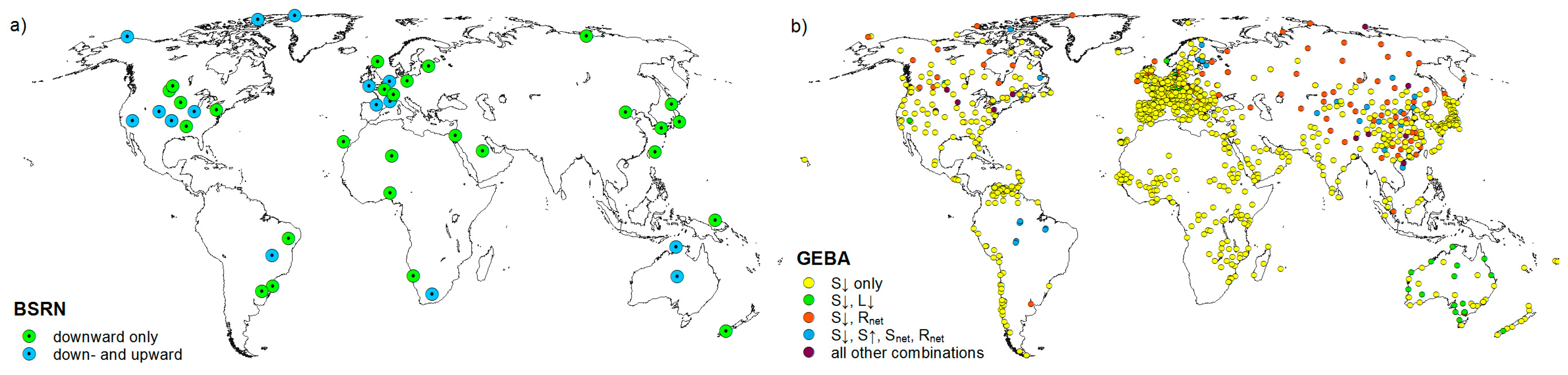
2.3.1. Baseline Surface Radiation Network (BSRN)

The Baseline Surface Radiation Network (BSRN) was an initiative from the World Climate Research Programme (WCRP) Radiative Fluxes Working Group and is now incorporated into the WCRP Global Energy and Water Cycle Experiment (GEWEX). The aim of BSRN is to collect and provide data from a high qualitative radiometric network. The number of stations is relatively low (Table 2) but shortwave and longwave surface radiation fluxes of “best possible quality currently available” are provided [22] (p. 6). BSRN data were downloaded via the data portal http://pangaea.de/ in 01/2015 as monthly means (calculated by the data warehouse tool) of all available radiation flux variables (if available). In cases where more than one sensor reported data values, we obtained the mean value. Some errors in the database (e.g., interchanged variables) were found, reported and are already being updated. Forty-three BSRN stations (Figure 1a) are located within the land-ocean mask of WaterGAP, providing data for at least 6 months within the analysis time (1992–2012) and could thus be used for this study (see Table 2 for a summary of number of stations/months).

2.3.2. Global Energy Balance Archive (GEBA)

In order to extend the geographical coverage of the evaluation sites, the Global Energy Balance Archive (GEBA) is used in addition to BSRN. GEBA contains long-time averaged surface radiation fluxes of more than 1500 stations worldwide. The data are quality controlled and coded with quality flags [23]. Station data were used if at least 6 monthly data values were available and quality flags indicated no problematic data (quality control procedure 1–4 have values > 4). Twenty GEBA stations were excluded as they provide monthly aggregates of BSRN stations. Figure 1b shows the location of the stations. The data were downloaded via http://www.geba.ethz.ch/ in August 2014. The coordinate was rounded to the next decimal point in case a GEBA station was located at the 0.5° grid cell border.

2.3.3. Calculation of Net Radiation and Its Components

Based on the monthly averages of the measurements, Snet (Lnet) radiation was calculated as S↓ minus S↑ (L↓ minus L↑) and Rnet as the sum of Snet and Lnet.

2.4. Efficiency Metrics

Efficiency metrics are used to quantify the goodness-of-fit between observations and simulations. There are numerous metrics available (each with benefits and limitations) and have been subject to reviews in the past e.g., [46,47]. Möller [48] analyzed WaterGAP model outputs with BSRN station data (from the four model variants, Table 1) by using ten efficiency metrics. She found that the Nash–Sutcliffe Efficiency and the Mean Absolute Error E M A E are the best metrics to reflect the characteristics of the modeled radiation vs. the simulated ones. The advantages of the Kling–Gupta Efficiency E K G , which builds on the Nash–Sutcliffe Efficiency, are the possibility to split this metric into the three components and to determine the dominant component [49]. In this study, E K G and its components, as well as E M A E , are used to assess the simulations with station observations.

2.4.1. Kling–Gupta Efficiency

Gupta et al. [49] and, later on, Kling et al. [50] decomposed the very popular Nash–Sutcliffe Efficiency metric into three components to allow diagnostic insights into the model performance and created the Kling–Gupta Efficiency metric by computing the Euclidian distance of the components from the ideal point ( E K G , Equation (6) in its version 2012 which is used here).
E K G = 1 ( E K G r 1 ) 2 + ( E K G b e t a 1 ) 2 + ( E K G g a m m a 1 ) 2
where E K G r is the correlation coefficient between simulated and observed values [-] and can act as indicator for the timing, E K G b e t a is the bias ratio (Equation (7)) [-] and can act as indicator if biases of the mean values occur and E K G g a m m a is the variability ratio (Equation (8)) [-] which can act as indicator for the variability of simulated (S) and observed (O) values.
E K G b e t a = μ S μ O ,
E K G g a m m a = C V S C V O = σ S / μ S σ O / μ O ,
where μ is the mean value (e.g., in Wm−2), σ is the standard deviation of the value (e.g., in Wm−2), C V is the coefficient of variation [-]. The optima of E K G and its components are one. The lowest component determines the E K G value. Furthermore, Gupta et al. [49] provided a methodology to assess the relative contribution g i of the three components as:
g i = G i j = 1 3 G j ,
with
G 1 = ( E K G r 1 ) 2 ,
G 2 = ( E K G g a m m a 1 ) 2 ,
G 3 = ( E K G b e t a 1 ) 2 .

2.4.2. Mean Absolute Error

An absolute measure of model efficiency is the Mean Absolute Error E M A E . It is calculated as the absolute difference between observed and simulated (monthly) data, which are then averaged over the number of observations (Equation (13)). A great advantage of this absolute efficiency criterion is the resulting number in the unit of measurement, which can then be used, for example, to assess absolute errors among the radiation components.
E M A E = 1 n i = 1 n | O i S i |
where O i is the observed (monthly) value for time step i and S i is the modeled (monthly) value of the variable.

2.4.3. Sum of Ranks

According to Möller [48], the model variants were ranked for the efficiency metrics, giving the value “1” for the model variant with the highest performance (maximum E K G or minimum E M A E , respectively) and incrementing values from the highest to lowest performing model variant. This is done for each station and then aggregated over the dataset. Finally, the model variant with the lowest rank can be seen as the best model variant amongst the data set and radiation component considered here.

3. Results and Discussion

In this section, we firstly compare the radiation components with observations from BSRN and GEBA datasets (Section 3.1). Then, we assess global averages and spatial differences of net radiation and its components (Section 3.2). Finally, we discuss the optimal radiation input and possible improvements in Section 3.3.

3.1. Comparison to Station Measurements

Monthly grid cell values generated from the different data sources (see Table 1) are compared with BSRN and GEBA ground measurements. The comparison results are evaluated and discussed using the efficiency metrics defined in Section 2.4.
Results are displayed as boxplots for the E K G criterion (Figure 2) as well as single components of E K G (Figure 3, Figure 4 and Figure 5) and for E M A E (Figure 6). The BSRN dataset is separated into one where all 43 stations are included (green color in the figures) and one with only the 16 stations where both components (upward, downward) are measured (blue color in the figures). Remarkable differences exist between the GEBA and BSRN comparison results for all radiation components (Figure 2 and Figure 6). For the downward components and both efficiency criteria, the simulations fit best to the subset of 16 BSRN stations, followed by all BSRN stations. Generally, lower performance is achieved for the GEBA stations, which is expected due to the larger data uncertainty [51]. However, due to the larger spatial coverage of this data set (at least for some components), integration of GEBA data allows a more robust assessment.
Analyzing Figure 2 and Figure 6, downward radiation components are represented with high performance by all model variants, indicated by the overall high value for E K G as well as (compared to net radiation) low E M A E of around 10 Wm−2 (slightly higher for S↓, lower for L↓). Except for PGFv2, S↓ has a mean bias ( E K G b e t a ) greater than one which relates to an overestimation compared to measurements and L↓ has a (slight) mean bias below one (Figure 3). This is in line with previous assessments [2,3]. L↑, as modeled by WaterGAP (all except ERAIN), has a lower performance (except E M A E and GEBA) than with ERAIN. Two possible reasons are that: (a) surface temperature as the main factor for L↑ calculation is strongly constrained by observations; or (b) emissivity values are more realistic in ERAIN.
Simulated S↑ is modeled with low agreement in comparison to observed values. The timing of S↑ (indicated by E K G r , Figure 4) is similar among the several forcings. The indicator of variability ( E K G g a m m a ) is underestimated more strongly by ERAIN compared to the simulated ones (Figure 5) but most differences among the forcings occur in mean bias ( E K G b e t a , Figure 3). For GEBA stations and simulated S↑, the mean bias E K G b e t a is greater than one. Besides the non-representative albedo and emissivity values of the surface beneath the measurement surface, obviously, different albedo values are responsible for different mean biases between simulations and reanalysis-based S↑ (compare ERAID and ERAIN for GEBA dataset of Figure 3).
There is no general best meteorological forcing for Snet. Due to the small footprint of upward radiation measurement, we did not expect better agreements. For example, if the area below the measurement consists of grassland but the majority of the 0.5° grid cell contains forest, the agreement is expected to be low due to the strongly differing albedo. For the BSRN stations, PGFv2 has the highest performance whilst for the GEBA stations WFDEI (and ERAID for E M A E ) ranks first (Table 3). The variability of net shortwave radiation is underestimated by all forcings, but to a lower degree by ERAIN (Figure 5). Differences in modeling L↑ are small (values close to optimum for E K G r and E K G b e t a ) to moderate ( E K G g a m m a ). Interestingly, for L↓, variability is likely to be overestimated by all model variants (except PGFv2 and BSRN) and the variability of L↑ is at the same time underestimated by the WaterGAP simulations. All model variants have a low performance for Lnet which is a result of differences in timing and variability (Figure 4 and Figure 5). ERAIN ranks first (for E M A E and GEBA together with WFDEI). However, the most important variable for calculating PET is Rnet. For the BSRN stations, the model variant WFDEI has the highest performance to observations; for GEBA stations, the PGFv2 variant ranks first in both cases followed by ERAIN. In terms of mean bias, Rnet is overestimated by the model variants, independently of the meteorological forcing (Figure 3). This is in agreement with Wild et al. [3], as they estimated a much lower value for the global land area (see Section 3.2, although Antarctica was included in their assessment). We assume that the overestimation of mean S↓ (Figure 3) is one reason for the high value of global land Rnet obtained in this study. The measure of variability (Figure 5) (and to a lesser extent timing, Figure 4) for Rnet varies by reference dataset. Nevertheless, the mean absolute biases for Rnet are with 15 to 20 Wm−2 being the highest deviation from all the components throughout the forcings.
Analyzing the relative contribution of the E K G components to the overall value (Figure 7), it can be stated that the correlation (thus the timing) contributes to the least extent (except S↑) for all radiation components. For the shortwave radiation components (and Rnet), the mean bias is dominating, whereas variability is dominating for the longwave components.

3.2. Intercomparison of Global-Scale Net Radiation and Its Components

Figure 8 shows simulated net radiation (bottom row) and its components from WFDEI and differences to the other model variants described in Table 1. It is worth noting that in northern Africa and Somalia, the Saudi-Arabian peninsula, central and Western Australia, as well as the Amazon and Mexico, Rnet of ERAIN is significantly lower than the current standard meteorological forcing of WFDEI (brown to red colors in Figure 8, bottom line). Despite large areas of lower Rnet values, there are numerous grid cells with drastically higher values for ERAIN compared to WFDEI (maximum difference in the Himalayan Mountains is 196 Wm−2). For long term (1979–2012) global land (except Antarctica) averages of net radiation, ERAIN has the highest values (83.0 Wm−2), compared to (slightly) lower values of the other forcings (PGFv2: 82.9 Wm−2, ERAID 82.0 Wm−2, WFDEI 81.0 Wm−2). Other estimates (that include Antarctica) are lower (e.g., 70 Wm−2, [3]).
Comparing WFDEI and ERAID (which differ in terms of the adjustments of Weedon et al. [8]), 40.2% of the global land area are within ±5 Wm−2 difference for Rnet, which shows a higher agreement when compared to the other forcings (PGFv2 35.1%, ERAIN 19.1%). Whereas higher (lower) Rnet values for ERAID are calculated in 36.2% (23.7%) of land area, a similar pattern, i.e., the tendency to calculate higher Rnet can be found for PGFv2 (37.2%, 27.8%) and ERAIN (48.9%, 32.0%). When separating the energy-limited and water-limited regions (Section 1), the forcing leads to pronounced differences. For ERAID and energy-limited (water-limited) regions, 34.3% (45.3%) of land area is within ±5 Wm−2 difference, with similar values for PGFv2 (38.3%, 32.3%) but are in much lower agreement with ERAIN (18.8%, 19.3%).
Rnet is larger than 5 Wm−2 in the percentage of land area for energy-limited/water-limited regions and ERAID (40.3%/32.6%) as well as PGFv2 (43.3%/31.9%). For ERAIN, 62.0% of energy-limited regions have Rnet values that are higher than 5 Wm−2 compared to WFDEI, whereas water-limited regions have, in the predominantly land area (43.2%), Rnet values that are lower than 5 Wm−2 (see also the spatial differences in Figure 8). Hence, by using ERAID or PGFv2 instead of WFDEI, around 1/3 (and for ERAIN around 1/2) of energy-limited regions could profit from an increasing amount of energy for evapotranspiration. Taken into account the different fraction of energy-limited/water-limited regions, on 18.7% to 28.8% of the global land area, the forcings ERAID, PGFv2 and ERAIN are calculated to have higher Rnet (compared to WFDEI) which would likely increase evapotranspiration. In contrast, on 8.6% to 11.8% on the global scale, Rnet decreases with the alternative forcing.
Absolute differences for the radiation components from WFDEI are also shown in Figure 8. Differences in S↓ for WFDEI compared to ERAID and ERAIN are low, but compared to PGFv2, WFDEI has 5 to 25 Wm−2 less S↓ in the US, northern Africa, Australia and the mountain regions in central Asia. In tropical regions, and to a lesser extent in northern Eurasia, S↓ is higher in WFD (Figure 8, first row). S↑ differences of WFDEI and ERAID are (except for small regions) within ±5 Wm−2, which is expected due to the smaller absolute values. As the land cover class dependent albedo values are comparable, WFDEI and PGFv2 differ with more than ±5 Wm−2 in areas where S↓ is differing, but to a much lesser extent. Most differences (between ±50 Wm−2) occur between WFDEI and ERAIN, which is interesting as S↓ is comparable. This could be related to a higher surface albedo of ERAIN that induces higher S↑. Other factors, e.g., clouds, might also contribute to the higher upward radiation, but no hints for an overestimation of cloudiness have been found by comparisons with BSRN stations in Europe and Africa [18]. Snet is very similar between WFDEI and ERAID, but differs from ERAIN (in general with lower values except the tropics) and PGFv2 (in general with higher values except for the tropics).
The pattern of differences between WFDEI to the other model variants for L↓ is similar in most regions; in the tropics, WFDEI has less L↓, whilst in most other regions, differences are within ±5 Wm−2 or, in the case of PGFv2, higher (up to 25 Wm−2) in most other regions. Differences > 5 Wm−2 can be found for L↑ only between WFDEI and ERAIN. Most of the dry regions have higher values in WFDEI (up to 50 Wm−2 for large areas), whereas the tropics (and Greenland) have lower values up to 25 Wm−2. The difference pattern for Lnet is diverse. ERAIN has, in general, smaller values for Lnet, especially in dry regions; ERAID has lower values in the tropics and PGFv2 has lower values in the tropics but higher values for most other areas. When comparing the differences of WFDEI to ERAIN and ERAID, the effect of modeling outgoing radiation within WaterGAP is visible. Based on an additional model run, where T from ERA-Interim (instead from WFDEI) was used for ERAID, we can summarize that T affects model results in only a minor manner and thus, differences in emissivity values (or other, ERA-Interim related characteristics) determine the difference between ERAIN and the WaterGAP calculations. The same results occur when T and P from WFDEI are used in a PGFv2 model run. Whereas the differences in the Amazon are comparable, ERAIN shows large differences in Africa, the Saudi-Arabian peninsula as well as Australia. For some regions, the calculation of outgoing radiation components in WaterGAP (ERAID, PGFv2) leads to changing signs of the differences compared to those obtained from ERAIN.
Summarizing the main findings of the inter-comparison of the four model variants, it can be stated that ERAIN has the highest net radiation at the global land scale and the standard forcing WFDEI the lowest. In energy-limited regions, the alternative forcings (especially ERAIN) have higher net radiation which has an influence on the evapotranspiration calculation. Especially for the downward components and PGFv2 as well as for the upward components and ERAIN, differences among the model variants are visible.

3.3. Discussion of Optimal Radiation Input

The downward components of all model variants show a high performance compared to the observed radiation apparent in Figure 2 (top row) but may still have systematic biases in terms of over and underestimation (Figure 3). According to the rank sums in Table 3 and S↓, highest performances are simulated when WaterGAP is forced by WFDEI, followed by PGFv2 and ERAID/ERAIN variants. The preparation and adjustments of WFDEI [8,29] to radiation fluxes from ERA-Interim reanalysis (see Section 2.1.2) lead to improved results for S↓, independently of the station dataset and efficiency criterion (Table 3). Interestingly, the E K G components, except E K G g a m m a (which is the dominant component (Figure 7) and thus influencing overall E K G value at most), perform worse than the directly obtained S↓ from ERA-Interim (Table 4 and Table 5). For L↓ (only elevation corrected), performance is worse for BSRN stations (except E K G g a m m a which is again the dominant component, Figure 7) but of the same quality for GEBA stations (Table 3). As the results of WFDEI are similar or better than ERAID (except for L↓ and BSRN), the thorough interpolation scheme of Weedon et al. [8] improved the quality of the meteorological forcing. The PGFv2 model variant ranks second for S↓ and BSRN and first for GEBA stations, whereas for L↓ the PGFv2 model variant is at the first position for both observation datasets (except for E K G and GEBA data) and can, therefore, be seen as a valuable alternative for downward radiation.
WaterGAP simulations of S↑ have a higher performance than those from ERAIN for the BSRN stations and a lower performance for WFDEI and ERAID for the GEBA stations consistently among the two efficiency criteria (Table 3 and Table 4). The calculation of S↑ in WaterGAP and underlying assumptions (e.g., albedo) are of the same quality as those from ERAIN for the grid cells where measurement data are available, even though the E K G values of S↑ are drastically lower compared to S↓. Due to the small footprint of upward radiation measurements (and thus the questionable representativeness for the 0.5° grid cell) as well as the low number of stations, this result may also be driven by chance. The E K G of L↑ is close to the optimum with highest performance with ERAIN for BSRN stations and for E K G also for GEBA stations (Table 3), whereas E K G b e t a and E K G r for all variants are close to optimum and the indicator of variability E K G g a m m a (which is dominant in E K G value) differs between the model variants (Figure 3, Figure 4, Figure 5 and Figure 7). For BSRN and GEBA stations, the WaterGAP calculation of L↑ variability E K G g a m m a has a higher performance compared to observations than those from ERAIN (Table 4 and Table 5). Even though, overall, the E K G value has a slightly weaker performance than those from ERAIN, the approach of WaterGAP using a land cover class based emissivity value to determine L↑ can be seen as plausible. However, here also, the small number of stations and months available for upward radiation components data (Table 2), as well as the small footprint for upward radiation measurement, limits the assessment. However, currently, the emissivity value is kept constant within WaterGAP which is a problem especially when land surface is covered by snow which influences emissivity values [52,53,54]. It should, therefore, be tested if a snow-cover-dependent emissivity value leads to improvements for WaterGAP calculation of L↑.
The evaluated Lnet performance depends largely on the efficiency metric applied. Whereas E K G values perform low for all model variants (Figure 2), values for E M A E are, compared to the other radiation fluxes, relatively low. The subtraction of two large values (L↓, L↑) leads to low absolute values (e.g., compared to Snet, Figure 8) and thus, absolute errors can be lower. On the other hand, small uncertainties in L↓ and L↑ are translated into large uncertainties for Lnet which is visible, e.g., for E K G b e t a (Figure 3).
For calculating PET, Rnet is the most important variable. The relative efficiency criterion E K G (Figure 2) is relatively low, independently of the model variant and the medians of absolute error E M A E are high with around 20 Wm−2. The rank sums for Rnet do not perform highest when substituting the upward radiation calculation of WaterGAP with those values obtained directly by ERA-Interim (Table 3). ERAIN has a higher performance than ERAID but for each efficiency criteria and station database, either WFDEI or PGFv2 perform better than ERAIN (Table 3). Snow dynamics are modeled within WaterGAP and albedo changes when snow cover is present [27]. Therefore, the use of ERAIN may induce inconsistent representation of land cover dependent parameters as albedo is also modeled by ERAIN. This, and the small benefit of using ERAIN, has to be considered when deciding about the optimal input.
WaterGAP uses a very simple scheme to calculate the energy balance at the surface. It uses only land-cover dependent albedo and emissivity values. The radiation transfer scheme that is integrated in ERA-Interim is highly complex, taken into account different bandwidths of radiation transfer, cloud (and atmosphere) properties and is designed to close the energy balance both at the surface and top level of the atmosphere [7]. Even so, in principle, ERA-Interim also considers surface albedo and emissivity and is therewith comparable in a very general sense, even though the processes are far more physically constrained.
All model variants have a positive mean bias for Rnet (Figure 3), which indicates that this variable is overestimated by about 20% compared to measurements. Consequently, E K G b e t a is the dominant component of the E K G value (Figure 7). Obviously, the higher E K G b e t a of S↓ propagates to Snet and Rnet (Figure 7) as this is described in the literature [2,3]. For the 16 BSRN stations, the current standard forcing of WaterGAP (WFDEI) provides the highest performance for both efficiency criteria (Table 3). For the 142 GEBA stations with net radiation data, the best match to simulations can be reached when using PGFv2 forcing (Table 3).
One of the foci of this study was to assess whether differences in results occur in energy- and water-limited areas. However, the discrepancy of the distribution of stations in energy limited vs. water limited regions (on average, only 28% of GEBA stations and 38% of BSRN stations are in water-limited grid cells) hinders a robust assessment of the performance in those distinct regions. Rank sums aggregated for BSRN and energy/water limited regions (not shown) indicate only slight deviations from those in Table 3.
The scale mismatch between (small scale) station observations and 0.5 ° grid cells results in uncertain comparison results. The median E M A E for S↓ from this study is about three times higher (10 to 15 Wm−2, Figure 6) than those of Hakuba et al. [26]. Obviously, due to the heterogeneity of land surface characteristics, the representativeness of downward and upward radiation fluxes differs fundamentally. However, monthly averaging can smear short-term (and small scale) atmospheric effects, which barley applies for land surface heterogeneities.
PET was calculated for the four model variants using the Priestley-Taylor approach [55] (Figure 9). In general, the difference patterns are similar to those of Rnet (Figure 8). Less PET, in comparison with WFDEI, occurs for all other model variants mainly in the tropics and for ERAIN in the very dry regions of Northern Africa and Australia. On a global scale, WFDEI has highest value for PET and the overall range among the model variants is about 24 mm·year−1 (lowest value for ERAIN). The highest absolute range (100 mm·year−1) among the models occurs in water limited grid cells, where WFDEI and ERAID have the same values and ERAIN the lowest. For the energy limited regions, WFDEI has the second lowest value (ERAIN has the highest) while the models vary by about 70 mm·year−1 (Table 6). As AET could be only increased in energy limited regions, this implies that WaterGAP would simulate higher AET when using ERAIN as radiation input.

4. Conclusions

In this study, we assessed the performance of radiation components in experiments with the global freshwater model WaterGAP on a 0.5° × 0.5° grid scale against station observations from the BSRN and GEBA databases. The model was driven with two state-of-the-art meteorological forcings (WFDEI and PGFv2) as well as with the interpolated downward radiation data from ERA-Interim reanalysis (ERAID) and finally a radiation dataset, including both downward and upward components from ERA-Interim (ERAIN). We used two efficiency metrics (one absolute, and one relative) for the comparison analysis. In addition, we assessed spatial differences among the radiation components as well as their effect on PET. The results can be summarized as follows:
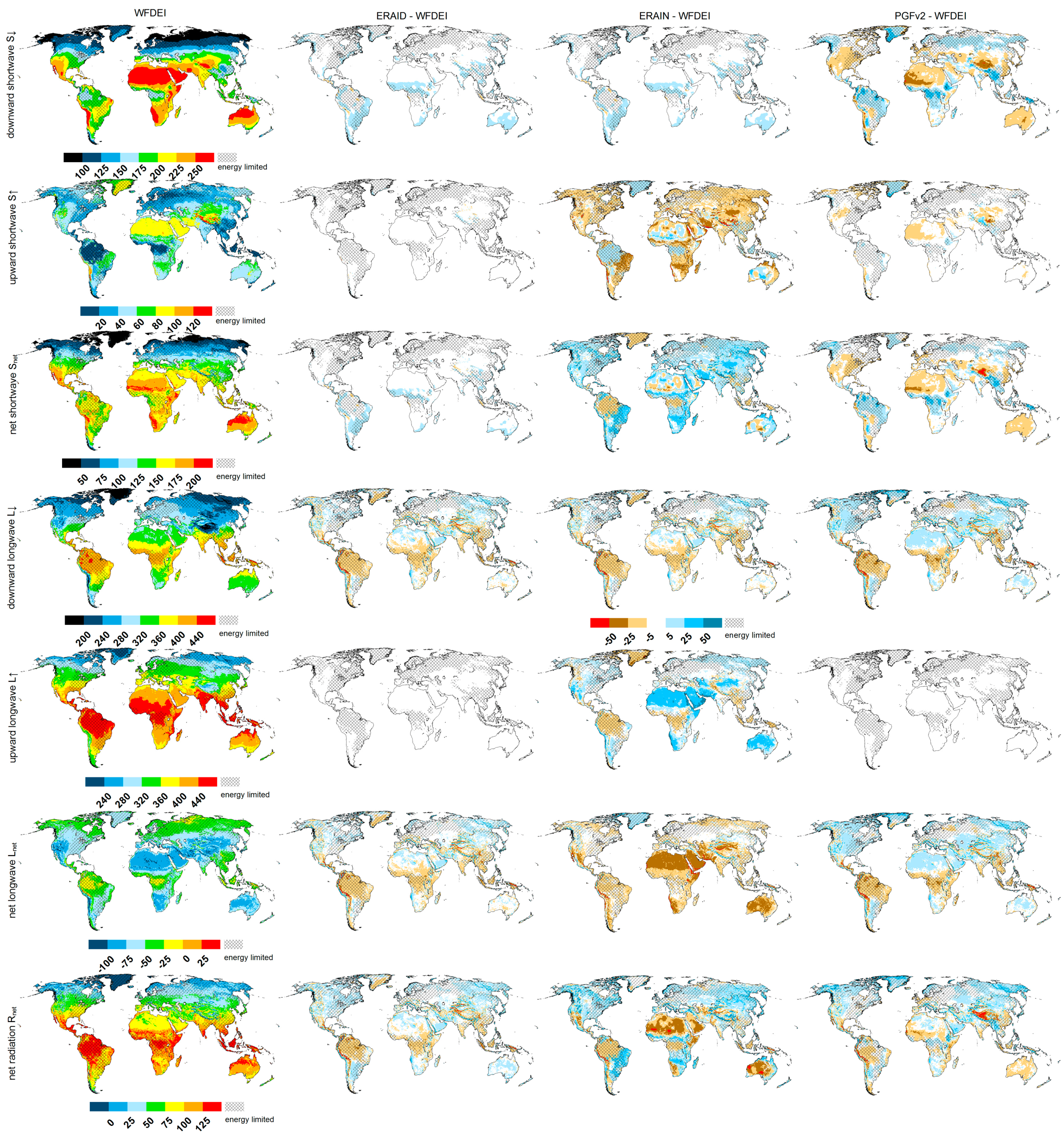
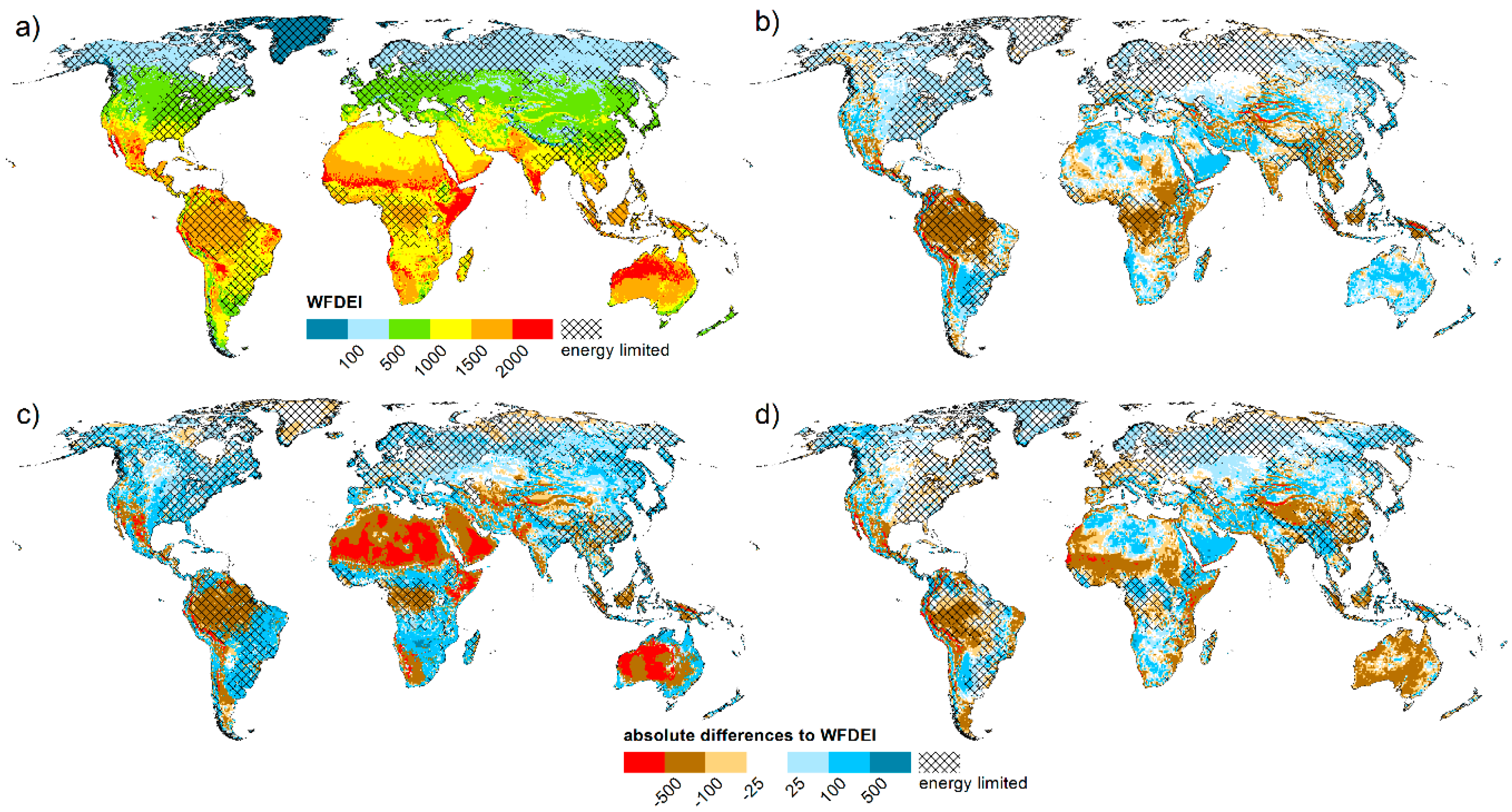
  • For global land averages, Rnet differs only slightly among the model variants (~2 Wm−2). However, regionally large differences of Rnet, S↑ and Lnet were found, especially in comparison with ERA-Interim reanalysis (Figure 8).
  • Rnet values of WaterGAP as forced by WFDEI is within ±5 Wm−2 agreement to the ERA-Interim reanalysis for 19.1% of the global land area, with similar numbers for energy-limited and water-limited regions.
  • In 62.0% of energy-limited regions (relates to 28.8% of the global land area), Rnet of the full radiation dataset from ERA-Interim is higher by more than 5 Wm−2 and has, therefore, the highest potential to increase the simulated evapotranspiration as compared to the other forcings.
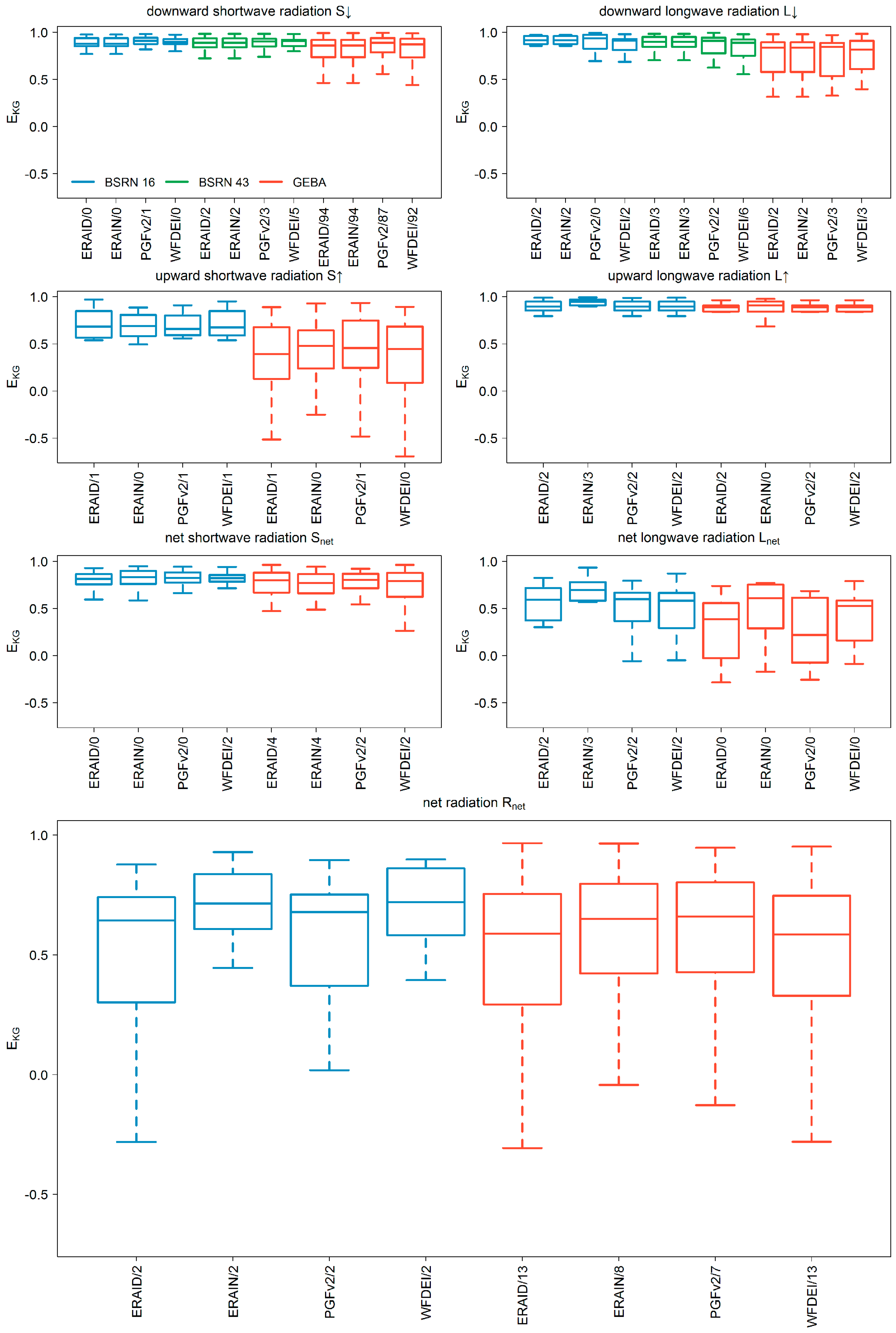
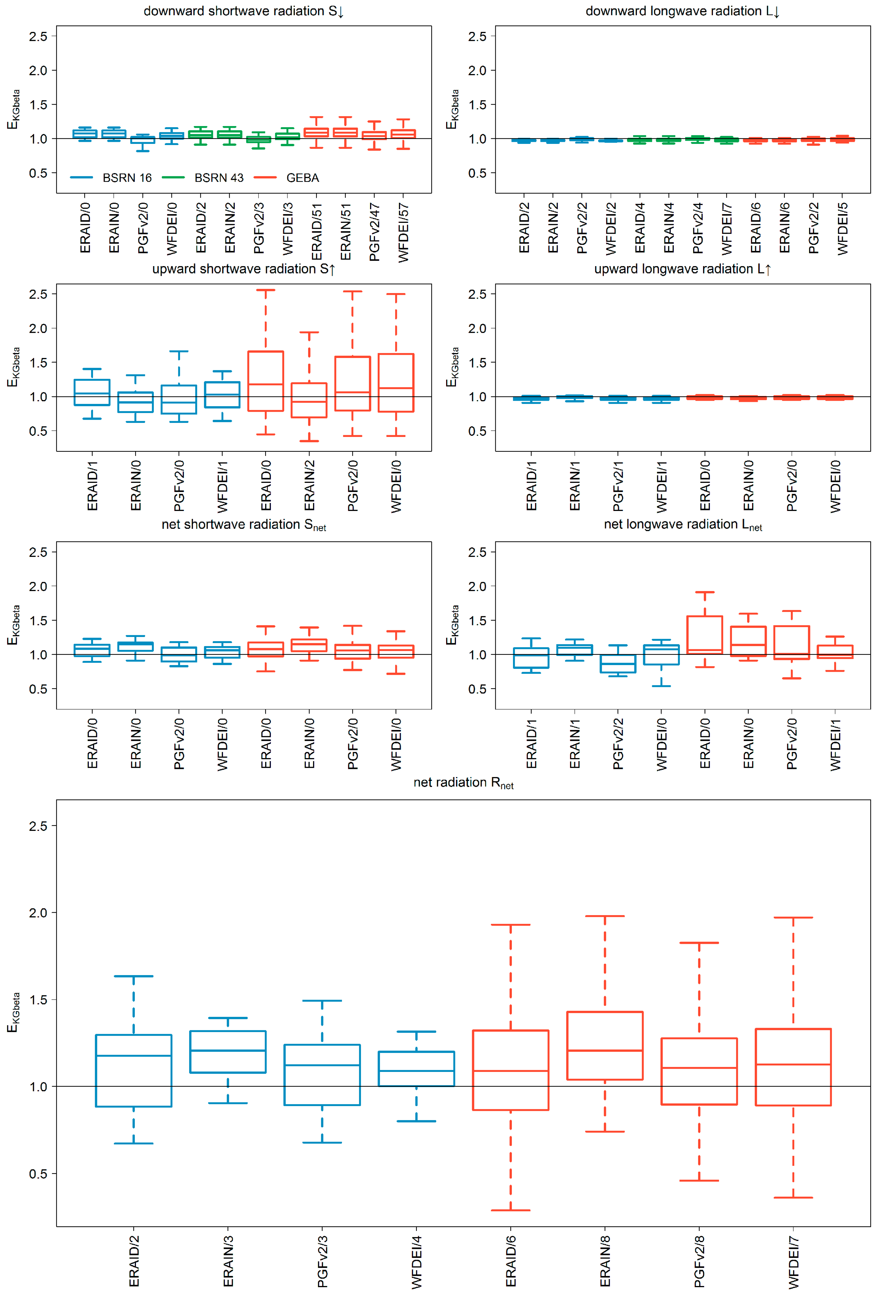
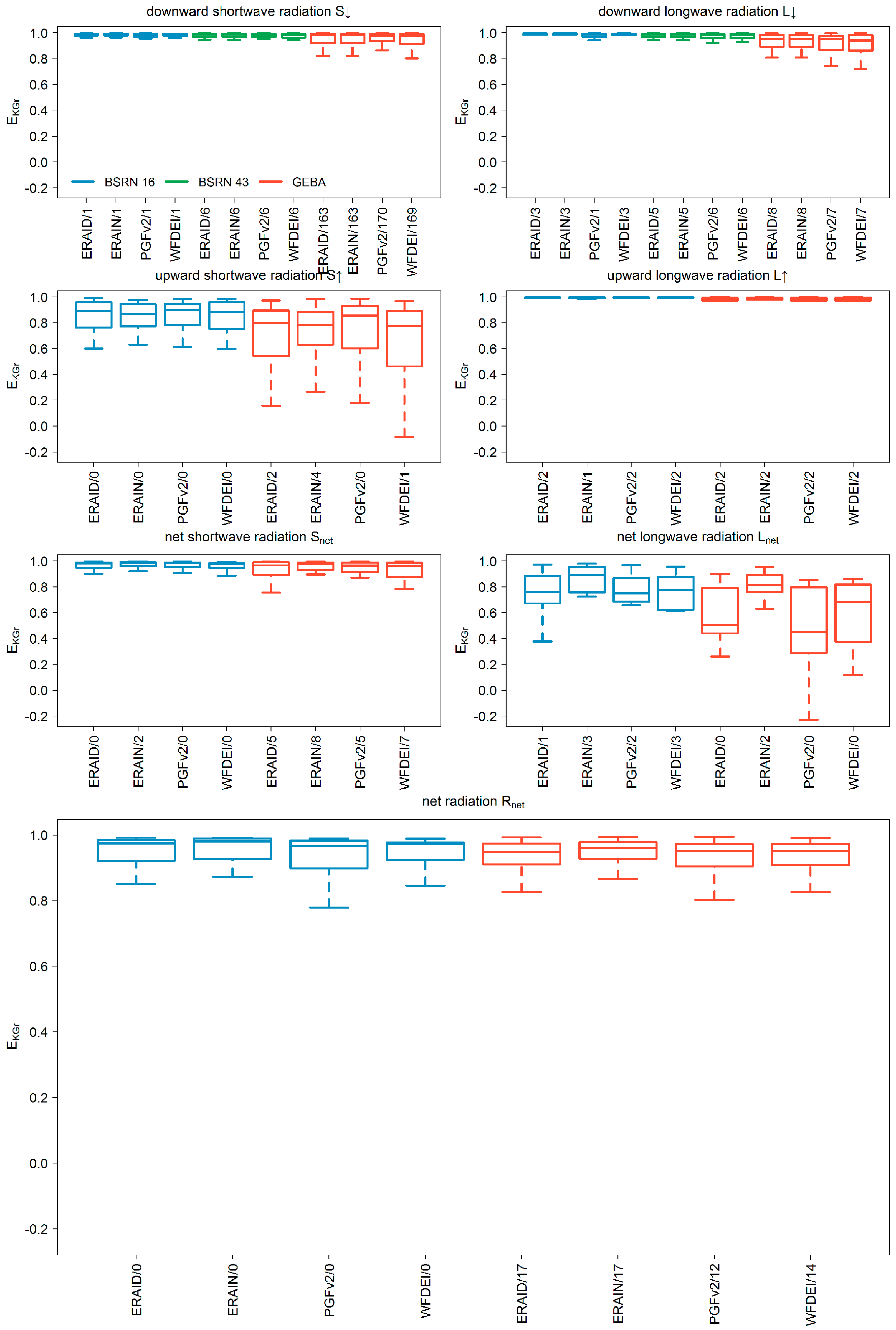
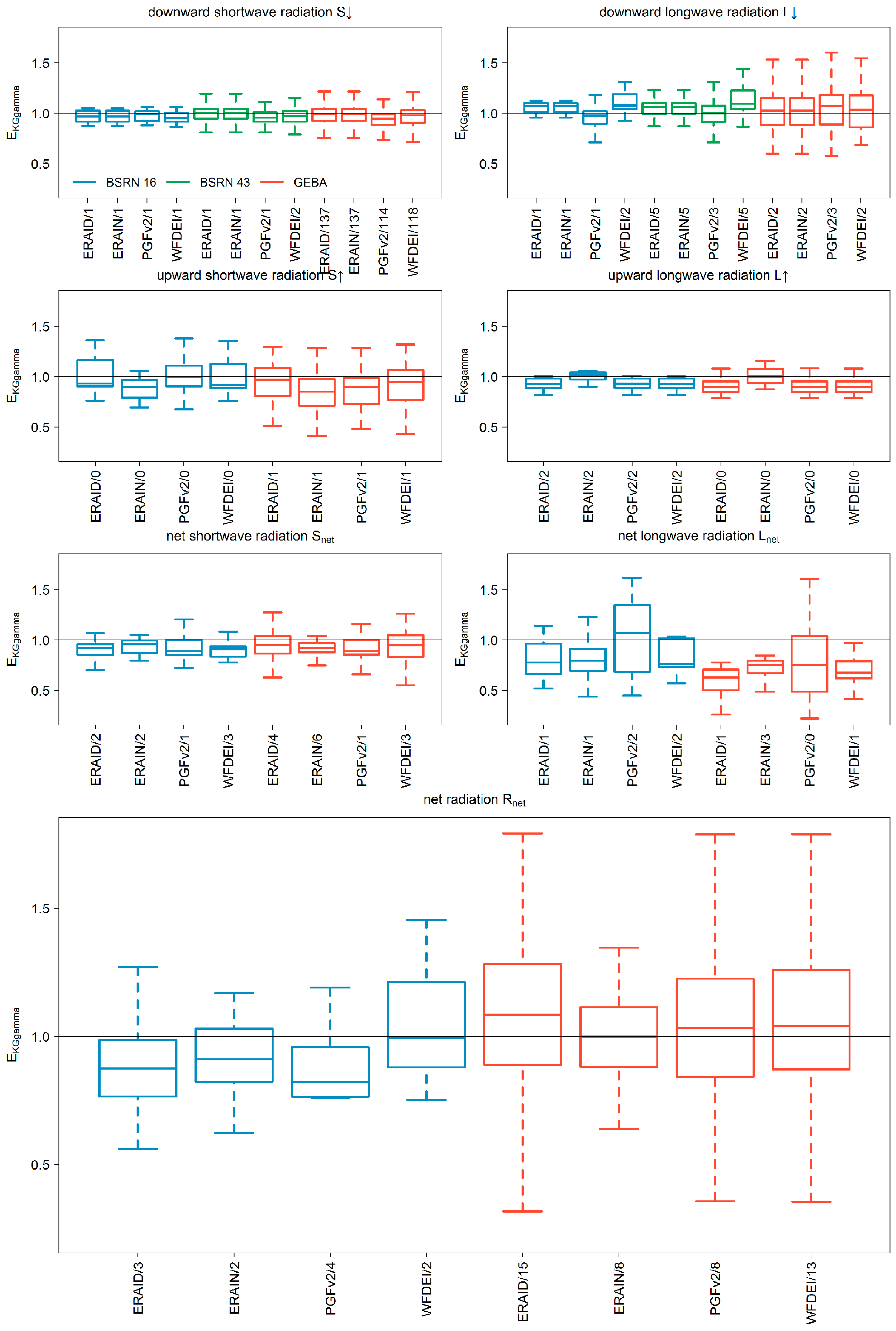
  • The downward radiation components of ERA-Interim show less or similar agreement to station observations compared to those from meteorological forcings (Table 3). The interpolation and correction approach of Weedon et al. [8] improves both downward radiation components (Table 3). However, for all model variants, a systematical overestimation of S↓ and Rnet was found when comparing to observation data.
  • The performance of S↑ radiation of ERA-Interim lies between the meteorological forcings WFDEI and PGFv2. For BSRN stations, the model variant where ERA-Interim downward components are used has a higher performance than the variant where also ERA-Interim upward components are used, whereas the opposite is true for GEBA stations. ERA-Interim values for L↑ are superior compared to those of WaterGAP except for the absolute error measure derived at the GEBA stations (Table 3).
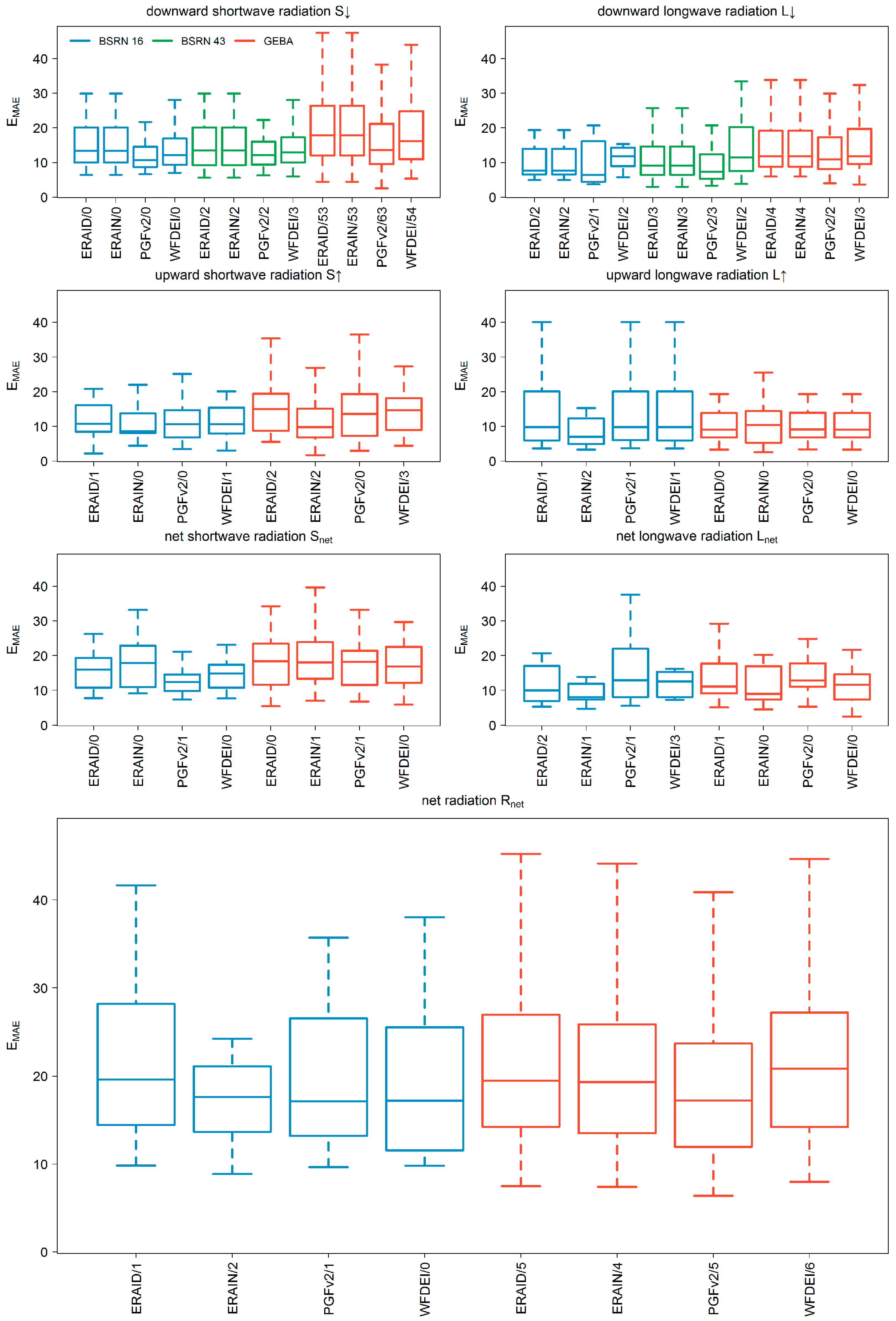
  • Best results for Rnet are found for current standard forcing (WFDEI, BSRN) or alternative forcing (PGFv2, GEBA) (Table 3), but median absolute errors are around 20 Wm−2 (comparable to the study of Troy and Wood [16]) and are mainly due to a higher mean value independent on the model variant (Figure 3 and Figure 4).
  • Global values for PET vary only by 25 mm·year−1 and the highest values are achieved with WFDEI forcing. However, in energy limited regions, where a change in PET directly influences AET, WFDEI has the second lowest value while ERAIN is 60 mm·year−1 higher.
Some limitations were found:
  • The relatively small number of some radiation measurements (e.g., 16 stations with upward flux measurements for BSRN) limits the overall assessment and hinders a robust assessment of the performance of the model variants, especially when separating into energy-limited/water-limited areas.
  • In contrast to the downward components, which show a reasonable representativeness of station measurements at the grid cell level [26], upward measurements have a small footprint and thus a high uncertainty in terms of representativeness for the grid cell.
The results imply a certain impact of radiation forcing and modeling on the simulation of PET, especially for energy-limited regions, which then affects the modeling of available water resources. However, calculation of PET can be done with many approaches which all have their own uncertainties. To quantify this, in particular, a study on the impact of PET (including different calculation approaches) is needed, followed by a quantification of the consequences for AET and freshwater resources. The results of this study can help to improve the understanding of net radiation estimates as an important driver of simulated evapotranspiration in GHMs. Even though this assessment is model-specific, GHMs with a comparable approach (i.e., land cover dependent albedo and emissivity) can benefit from this analysis as two of the most frequently used meteorological forcings and one reanalysis for two radiation setups were evaluated.

Acknowledgments

We thank Petra Döll for initial discussions according to the study design and Melanie Seeger (Möller before marriage) for her input regarding the efficiency criteria. We greatly appreciate the suggestions of three anonymous reviewers that helped to improve the manuscript significantly.

Author Contributions

Hannes Müller Schmied designed the study, performed the research, prepared the data and ran the model, analyzed the model output, created figures and tables and wrote the paper. All authors contributed to discussions and manuscript revision.

Conflicts of Interest

The authors declare no conflict of interest.

References

  1. Trenberth, K.E.; Fasullo, J.T.; Kiehl, J. Earth’s global energy budget. Bull. Am. Meteorol. Soc. 2009, 90, 311–323. [Google Scholar] [CrossRef]
  2. Wild, M.; Folini, D.; Schär, C.; Loeb, N.; Dutton, E.G.; König-Langlo, G. The global energy balance from a surface perspective. Clim. Dyn. 2013, 40, 3107–3134. [Google Scholar] [CrossRef]
  3. Wild, M.; Folini, D.; Hakuba, M.Z.; Schär, C.; Seneviratne, S.I.; Kato, S.; Rutan, D.; Ammann, C.; Wood, E.F.; König-Langlo, G.; et al. The energy balance over land and oceans: An assessment based on direct observations and CMIP5 climate models. Clim. Dyn. 2015, 44, 3393–3429. [Google Scholar] [CrossRef]
  4. Wild, M.; Liepert, B. The Earth radiation balance as driver of the global hydrological cycle. Environ. Res. Lett. 2010, 5. [Google Scholar] [CrossRef]
  5. Sood, A.; Smakhtin, V. Global hydrological models: A review. Hydrol. Sci. J. 2014, 60, 549–565. [Google Scholar] [CrossRef]
  6. Bierkens, M.F.P. Global hydrology 2015: State, trends, and directions. Water Resour. Res. 2015, 51, 4923–4947. [Google Scholar] [CrossRef]
  7. Dee, D.P.; Uppala, S.M.; Simmons, A.J.; Berrisford, P.; Poli, P.; Kobayashi, S.; Andrae, U.; Balmaseda, M.A.; Balsamo, G.; Bauer, P.; et al. The ERA-Interim reanalysis: Configuration and performance of the data assimilation system. Q. J. R. Meteorol. Soc. 2011, 137, 553–597. [Google Scholar] [CrossRef]
  8. Weedon, G.P.; Balsamo, G.; Bellouin, N.; Gomes, S.; Best, M.J.; Viterbo, P. The WFDEI meteorological forcing data set: WATCH Forcing Data methodology applied to ERA-Interim reanalysis data. Water Resour. Res. 2014, 50, 7505–7514. [Google Scholar] [CrossRef]
  9. Sheffield, J.; Goteti, G.; Wood, E.F. Development of a 50-year high-resolution global dataset of meteorological forcings for land surface modeling. J. Clim. 2006, 19, 3088–3111. [Google Scholar] [CrossRef]
  10. Müller Schmied, H.; Adam, L.; Eisner, S.; Fink, G.; Flörke, M.; Kim, H.; Oki, T.; Portmann, F.T.; Reinecke, R.; Riedel, C.; et al. Variations of global and continental water balance components as impacted by climate forcing uncertainty and human water use. Hydrol. Earth Syst. Sci. 2016, 20, 2877–2898. [Google Scholar] [CrossRef]
  11. Nasonova, O.N.; Gusev, Y.M.; Kovalev, Y.E. Impact of uncertainties in meteorological forcing data and land surface parameters on global estimates of terrestrial water balance components. Hydrol. Process. 2011, 25, 1074–1090. [Google Scholar] [CrossRef]
  12. Biemans, H.; Hutjes, R.W.A.; Kabat, P.; Strengers, B.J.; Gerten, D.; Rost, S. Effects of precipitation uncertainty on discharge calculations for main river basins. J. Hydrometeorol. 2009, 10, 1011–1025. [Google Scholar] [CrossRef]
  13. Döll, P.; Douville, H.; Güntner, A.; Müller Schmied, H.; Wada, Y. Modelling freshwater resources at the global scale: Challenges and prospects. Surv. Geophys. 2016, 37, 195–221. [Google Scholar] [CrossRef]
  14. Wild, M.; Ohmura, A.; Gilgen, H.; Morcrette, J.-J. The distribution of solar energy at the Earth’s sufrace as calculated in the ECMWF re-analysis. Geophys. Res. Lett. 1998, 25, 4373–4376. [Google Scholar] [CrossRef]
  15. Wild, M.; Ohmura, A.; Gilgen, H.; Morcrette, J.-J.; Slingo, A. Evaluation of downward longwave radiation in General Circulation Models. J. Clim. 2001, 14, 3227–3239. [Google Scholar] [CrossRef]
  16. Troy, T.J.; Wood, E.F. Comparison and evaluation of gridded radiation products across northern Eurasia. Environ. Res. Lett. 2009, 4. [Google Scholar] [CrossRef]
  17. Jin, Y.; Randerson, J.T.; Goulden, M.L. Continental-scale net radiation and evapotranspiration estimated using MODIS satellite observations. Remote Sens. Environ. 2011, 115, 2302–2319. [Google Scholar] [CrossRef]
  18. Posselt, R.; Mueller, R.W.; Stöckli, R.; Trentmann, J. Remote sensing of solar surface radiation for climate monitoring—The CM-SAF retrieval in international comparison. Remote Sens. Environ. 2012, 118, 186–198. [Google Scholar] [CrossRef]
  19. Gómez, I.; Caselles, V.; Estrela, M. Seasonal Characterization of Solar Radiation Estimates Obtained from a MSG-SEVIRI-Derived Dataset and a RAMS-Based Operational Forecasting System over the Western Mediterranean Coast. Remote Sens. 2016, 8. [Google Scholar] [CrossRef]
  20. Inamdar, A.; Guillevic, P. Net surface shortwave radiation from GOES imagery—Product evaluation using ground-based measurements from SURFRAD. Remote Sens. 2015, 7, 10788–10814. [Google Scholar] [CrossRef]
  21. Boilley, A.; Wald, L. Comparison between meteorological re-analyses from ERA-Interim and MERRA and measurements of daily solar irradiation at surface. Renew. Energy 2015, 75, 135–143. [Google Scholar] [CrossRef] [Green Version]
  22. König-Langlo, G.; Sieger, R.; Schmithüsen, H.; Bücker, A.; Richter, F.; Dutton, E.G. Baseline Surface Radiation Network (BSRN) Update of the Technical Plan for BSRN Data Management; WCRP Report 24/2013; World Meteorological Organization (WMO): Geneva, Switzerland, 2013. [Google Scholar]
  23. Gilgen, H.; Ohmura, A. The Global Energy Balance Archive. Bull. Am. Meteorol. Soc. 1999, 80, 831–850. [Google Scholar] [CrossRef]
  24. Heinemann, G.; Kerschgens, M. Simulation of surface energy fluxes using high-resolution non-hydrostatic simulations and comparisons with measurements for the LITFASS-2003 experiment. Bound.-Layer Meteorol. 2006, 121, 195–220. [Google Scholar] [CrossRef]
  25. Horlacher, V.; Osborne, S.; Price, J.D. Comparison of two closely located meteorological measurement sites and consequences for their areal representativity. Bound.-Layer Meteorol. 2012, 142, 469–493. [Google Scholar] [CrossRef]
  26. Hakuba, M.Z.; Folini, D.; Sanchez-Lorenzo, A.; Wild, M. Spatial representativeness of ground-based solar radiation measurements-Extension to the full Meteosat disk. J. Geophys. Res. Atmos. 2014, 119, 11760–11771. [Google Scholar] [CrossRef]
  27. Müller Schmied, H.; Eisner, S.; Franz, D.; Wattenbach, M.; Portmann, F.T.; Flörke, M.; Döll, P. Sensitivity of simulated global-scale freshwater fluxes and storages to input data, hydrological model structure, human water use and calibration. Hydrol. Earth Syst. Sci. 2014, 18, 3511–3538. [Google Scholar] [CrossRef]
  28. Budyko, M.I. Climate and Life; Academic Press: New York, NY, USA, 1974. [Google Scholar]
  29. Weedon, G.P.; Gomes, S.; Viterbo, P.; Shuttleworth, W.J.; Blyth, E.; Österle, H.; Adam, J.C.; Bellouin, N.; Boucher, O.; Best, M. Creation of the WATCH Forcing Data and its use to assess global and regional reference crop evaporation over land during the twentieth century. J. Hydrometeorol. 2011, 12, 823–848. [Google Scholar] [CrossRef]
  30. ECMWF IFS Documentation—Cy40r1 Part IV: Physical Processes; European Centre for Medium-Range Weather Forecasts: Reading, UK, 2014.
  31. Uppala, S.M.M.; KÅllberg, P.W.; Simmons, A.J.; Andrae, U.; Bechtold, V.D.C.; Fiorino, M.; Gibson, J.K.; Haseler, J.; Hernandez, A.; Kelly, G.A.; et al. The ERA-40 re-analysis. Q. J. R. Meteorol. Soc. 2005, 131, 2961–3012. [Google Scholar] [CrossRef]
  32. Stocker, T.F.; Qin, D.; Plattner, G.-K.; Tignor, M.; Allen, S.K.; Boschung, J.; Nauels, A.; Xia, Y.; Bex, V.; Midgley, P.M. (Eds.) IPCC Climate Change 2013: The Physical Science Basis. Contribution of Working Group I to the Fifth Assessment Report of the Intergovernmental Panel on Climate Change; Cambridge University Press: Cambridge, UK; New York, NY, USA, 2013.
  33. Harris, I.; Jones, P.D.; Osborn, T.J.; Lister, D.H. Updated high-resolution grids of monthly climatic observations—The CRU TS3.10 Dataset. Int. J. Climatol. 2014, 34, 623–642. [Google Scholar] [CrossRef] [Green Version]
  34. Döll, P.; Kaspar, F.; Lehner, B. A global hydrological model for deriving water availability indicators: Model tuning and validation. J. Hydrol. 2003, 270, 105–134. [Google Scholar] [CrossRef]
  35. Alcamo, J.; Döll, P.; Henrichs, T.; Kaspar, F.; Lehner, B.; Rösch, T.; Siebert, S. Development and testing of the WaterGAP 2 global model of water use and availability. Hydrol. Sci. J. 2003, 48, 317–337. [Google Scholar] [CrossRef]
  36. Döll, P.; Fiedler, K.; Zhang, J. Global-scale analysis of river flow alterations due to water withdrawals and reservoirs. Hydrol. Earth Syst. Sci. 2009, 13, 2413–2432. [Google Scholar] [CrossRef]
  37. Döll, P.; Fiedler, K. Global-scale modeling of groundwater recharge. Hydrol. Earth Syst. Sci. 2008, 12, 863–885. [Google Scholar] [CrossRef]
  38. Döll, P.; Müller Schmied, H.; Schuh, C.; Portmann, F.T.; Eicker, A. Global-scale assessment of groundwater depletion and related groundwater abstractions: Combining hydrological modeling with information from well observations and GRACE satellites. Water Resour. Res. 2014, 50, 5698–5720. [Google Scholar] [CrossRef]
  39. Haddeland, I.; Clark, D.B.; Franssen, W.; Ludwig, F.; Voß, F.; Arnell, N.W.; Bertrand, N.; Best, M.; Folwell, S.; Gerten, D.; et al. Multimodel estimate of the global terrestrial water balance: Setup and first results. J. Hydrometeorol. 2011, 12, 869–884. [Google Scholar] [CrossRef]
  40. Schewe, J.; Heinke, J.; Gerten, D.; Haddeland, I.; Arnell, N.W.; Clark, D.B.; Dankers, R.; Eisner, S.; Fekete, B.M.; Colón-González, F.J.; et al. Multimodel assessment of water scarcity under climate change. Proc. Natl. Acad. Sci. USA 2014, 111, 3245–3250. [Google Scholar] [CrossRef] [PubMed] [Green Version]
  41. Hagemann, S.; Chen, C.; Clark, D.B.; Folwell, S.; Gosling, S.N.; Haddeland, I.; Hanasaki, N.; Heinke, J.; Ludwig, F.; Voss, F.; et al. Climate change impact on available water resources obtained using multiple global climate and hydrology models. Earth Syst. Dyn. 2013, 4, 129–144. [Google Scholar] [CrossRef]
  42. Döll, P.; Müller Schmied, H. How is the impact of climate change on river flow regimes related to the impact on mean annual runoff? A global-scale analysis. Environ. Res. Lett. 2012, 7. [Google Scholar] [CrossRef]
  43. Portmann, F.T.; Döll, P.; Eisner, S.; Flörke, M. Impact of climate change on renewable groundwater resources: Assessing the benefits of avoided greenhouse gas emissions using selected CMIP5 climate projections. Environ. Res. Lett. 2013, 8. [Google Scholar] [CrossRef]
  44. Alcamo, J.; Leemans, R.; Kreileman, E. Global Change Scenarios of the 21st Century—Results from the IMAGE 2.1 Model; Pergamon: Oxford, UK, 1998. [Google Scholar]
  45. Wilber, A.C.; Kratz, D.P.; Gupta, S.K. Surface Emissivity Maps for Use in Satellite Retrievals of Longwave Radiation; NASA/TP-1999-209362; Langley Research Center: Hampton, VA, USA, 1999; 35p. [Google Scholar]
  46. Legates, D.R.; McCabe, G.J. Evaluating the use of “goodness-of-fit” Measures in hydrologic and hydroclimatic model validation. Water Resour. Res. 1999, 35, 233–241. [Google Scholar] [CrossRef]
  47. Krause, P.; Boyle, D.P.; Bäse, F. Comparison of different efficiency criteria for hydrological model assessment. Adv. Geosci. 2005, 5, 89–97. [Google Scholar] [CrossRef]
  48. Möller, M.I. Vergleich von Modellierten Globalskaligen Rasterdaten der Strahlung Mit Stationsbasierten Messwerten: Methodenentwicklung und Analyse. Master’s Thesis, Goethe-University Frankfurt, Frankfurt, Germany, 16 July 2015. [Google Scholar]
  49. Gupta, H.V.; Kling, H.; Yilmaz, K.K.; Martinez, G.F. Decomposition of the mean squared error and NSE performance criteria: Implications for improving hydrological modelling. J. Hydrol. 2009, 377, 80–91. [Google Scholar] [CrossRef]
  50. Kling, H.; Fuchs, M.; Paulin, M. Runoff conditions in the upper Danube basin under an ensemble of climate change scenarios. J. Hydrol. 2012, 424–425, 264–277. [Google Scholar] [CrossRef]
  51. Raschke, E.; Kinne, S.; Stackhouse, P.W. GEWEX Radiative Flux Assessment (RFA) Volume 1: Assessment. A Project of the World Climate Research Programme Global Energy and Water Cycle Experiment (GEWEX) Radiation Panel; WCRP Report 19/2012; World Meteorological Organization (WMO): Geneva, Switzerland, 2012. [Google Scholar]
  52. Russak, V.; Niklus, I. Longwave radiation at the earth’s surface in Estonia. Proc. Estonian Acad. Sci. 2015, 64, 480. [Google Scholar] [CrossRef]
  53. Hori, M.; Aoki, T.; Tanikawa, T.; Motoyoshi, H.; Hachikubo, A.; Sugiura, K.; Yasunari, T.J.; Eide, H.; Storvold, R.; Nakajima, Y.; et al. In-situ measured spectral directional emissivity of snow and ice in the 8–14 μm atmospheric window. Remote Sens. Environ. 2006, 100, 486–502. [Google Scholar] [CrossRef]
  54. Warren, S.G. Optical properties of snow. Rev. Geophys. 1982, 20, 67–89. [Google Scholar] [CrossRef]
  55. Priestley, C.H.B.; Taylor, R.J. Assessment of surface heat flux and evaporation using large-scale parameters. Mon. Weather Rev. 1972, 100, 81–92. [Google Scholar] [CrossRef]
Figure 1. Location of the reference stations used for evaluating the radiation components: Baseline Surface Radiation Network (BSRN), (a) and Global Energy Balance Archive (GEBA); (b) A specific color for GEBA stations was assigned when the radiation variable(s) were available for at least ten stations, otherwise joined to “all other combinations”.
Water 08 00450 g001
Figure 2. Validation of monthly radiation components with measurements of 16 BSRN stations (where all components are measured, blue color), 43 BSRN stations where only downward components were measured (green color) for the time period 1992–2012, as well as GEBA stations (red color) for the time period 1979–2012 using Kling–Gupta Efficiency E K G (-). Numbers after the slash indicate the number of stations that are outside of the 1.5 × inter quartile range and thus not included in the boxplot. Significant differences of metric distribution (two sample Kolmogorov–Smirnov test, p < 0.05) are present for GEBA stations and shortwave downward radiation for all combinations except ERAID-ERAIN. For single components of E K G , see Figure 3, Figure 4 and Figure 5.
Water 08 00450 g002
Figure 3. Validation of monthly radiation components with measurements of 16 BSRN stations (where all components are measured, blue color), 43 BSRN stations where only downward components were measured (green color) for the time period 1992–2012, as well as GEBA stations (red color) for the time period 1979–2012 using Kling–Gupta Efficiency component E K G b e t a (-) as indicator for mean bias. Numbers after the slash indicate the number of stations that are outside of the 1.5 × inter quartile range and thus not included in the boxplot. Significant differences of metric distribution (two sample Kolmogorov–Smirnov test, p < 0.05) are present for BSRN stations and the downward components for all combinations with PGFv2 and for the net shortwave as well as net longwave radiation for ERAIN-PGFv2. Within GEBA stations, significant differences occur for shortwave downward radiation between ERAIN/ERAID and PGFv2/WFDEI and also PGFv2-WFDEI; for net shortwave radiation between ERAIN-WFDEI and for net radiation between ERAID-ERAIN, ERAIN-PGFv2 and ERAIN-WFDEI.
Water 08 00450 g003
Figure 4. Validation of monthly radiation components with measurements of 16 BSRN stations (where all components are measured, blue color), 43 BSRN stations where only downward components were measured (green color) for the time period 1992–2012, as well as GEBA stations (red color) for the time period 1979–2012 using Kling–Gupta Efficiency component E K G r (-) as indicator for correlation, thus timing. Numbers after the slash indicate the number of stations that are outside of the 1.5 × inter quartile range and thus not included in the boxplot. Significant differences of metric distribution (two sample Kolmogorov–Smirnov test, p < 0.05) are present for GEBA stations and shortwave downward radiation for ERAID-WFDEI and ERAIN-WFDEI.
Water 08 00450 g004
Figure 5. Validation of monthly radiation components with measurements of 16 BSRN stations (where all components are measured, blue color), 43 BSRN stations where only downward components were measured (green color) for the time period 1992–2012, as well as GEBA stations (red color) for the time period 1979–2012 using Kling–Gupta Efficiency component E K G g a m m a (-) as indicator for variability. Numbers after the slash indicate the number of stations that are outside of the 1.5 × inter quartile range and thus not included in the boxplot. Significant differences of metric distribution (two sample Kolmogorov–Smirnov test, p < 0.05) are present for BSRN stations and longwave downward radiation for all combinations with PGFv2, for longwave upward radiation for ERAID-ERAIN, ERAIN-PGFv2 and ERAIN-WFDEI as well as for net radiation between PGFv2 and WFDEI. For the GEBA stations, significant differences occur for shortwave downward radiation among all combinations (except ERAID-ERAIN), and for longwave upward as well as for net radiation between ERAID-ERAIN, ERAIN-PGFV2 and ERAIN-WFDEI.
Water 08 00450 g005
Figure 6. Validation of monthly radiation components with measurements of 16 BSRN stations (where all components are measured, blue color), 43 BSRN stations where only downward components were measured (and green color) for the time period 1992–2012, as well as GEBA stations (red color) for the time period 1979–2012 using Mean Absolute Error E M A E (Wm−2). Numbers after the slash indicate the number of stations that are outside of the 1.5 × inter quartile range and thus not included in the boxplot.
Water 08 00450 g006
Figure 7. The average fraction of E K G component (-) showing the different contribution of correlation, variability and mean bias to the overall efficiency criteria.
Water 08 00450 g007
Figure 8. Average radiation components for 1980–2009 for WFDEI (1st column) and differences for ERAID-WFDEI (2nd), ERAIN-WFDEI (3rd) and PGFv2-WFDEI (last column). All units in Wm−2. Cross-hatched areas are energy limited areas after the Budyko approach, taken from the STANDARD model run of [27].
Water 08 00450 g008
Figure 9. Long term (1980–2009) average of potential evapotranspiration as calculated by the Priestley–Taylor approach for WFDEI (a); and differences for ERAID-WFDEI (b); ERAIN-WFDEI (c); and PGFv2-WFDEI (d) (all units in mm·year−1).
Water 08 00450 g009
Table 1. Model variant names for the experiment and source for climate variables. Abbreviations: S↓: shortwave downward radiation, S↑: shortwave upward radiation, L↓: longwave downward radiation; L↑: longwave upward radiation; P: precipitation; T: temperature; WaterGAP: Water—Global Assessment and Prognosis; WFDEI: WATCH Forcing Data methodology applied to ERA-Interim reanalysis; PGFv2: Princeton Global Meteorological Forcing Dataset version 2. Name for downward ERA-Interim radiation components is ERAID, for the variant where also upward ERA-Interim radiation is used, ERAIN.
NameS↓S↑L↓L↑P, T
WFDEIWFDEIWaterGAPWFDEIWaterGAPWFDEI
ERAIDERA-InterimWaterGAPERA-InterimWaterGAPWFDEI
ERAINERA-InterimERA-InterimERA-InterimERA-InterimWFDEI
PGFv2PGFv2WaterGAPPGFv2WaterGAPPGFv2
Table 2. Number of stations and months of the radiation data used within this study. Stations were only considered if at least 6 months of data were available.
Variable# Stations# Stations (Calculated)# Months# Months (Calculated)
BSRN
S↓43 5099
S↑16 2317
Snet 16 2289
L↓43 4872
L↑16 2210
Lnet 16 2205
Rnet 16 2171
GEBA
S↓1061 171,169
S↑43 3067
Snet 40 2791
L↓42 2933
L↑14 839
Lnet 13 692
Rnet142 11,525
Table 3. Rank sums divided by number of stations for the radiation components of BSRN and GEBA stations and the efficiency metrics E K G and E M A E . The lowest rank is shown in bold font, indicating the best match to observations. Model variants are abbreviated with ERD (stands for ERAID), ERN (ERAIN), PGF (PGFv2), WFD (WFDEI) and net radiation components with a subscript “n”.
BSRNGEBA
E K G E M A E E K G E M A E
ERDERNPGFWFDERDERNPGFWFDERDERNPGFWFDERDERNPGFWFD
S↓2.82.82.61.82.82.82.32.12.82.82.02.42.92.92.02.3
S↑2.22.53.02.32.32.73.02.03.02.31.92.93.02.02.03.0
Sn3.02.32.52.23.03.21.32.52.32.62.62.52.42.62.62.4
L↓2.42.42.42.92.42.41.83.42.52.52.62.52.62.62.22.6
L↑2.62.02.82.62.62.02.82.62.52.12.82.52.12.53.42.1
Ln2.81.53.22.52.21.73.52.73.01.53.02.52.82.13.02.1
Rn3.22.22.72.03.02.82.22.02.82.42.22.62.52.52.32.7
Table 4. Rank sums divided by number of stations for the radiation components, BSRN stations and the efficiency metrics E K G r , E K G b e t a and E K G g a m m a . The lowest rank is shown in bold font, indicating the best match to observations. Model variants are abbreviated with ERD (stands for ERAID), ERN (ERAIN), PGF (PGFv2), WFD (WFDEI) and net radiation components with a subscript “n”.
E K G r E K G b e t a E K G g a m m a
ERDERNPGFWFDERDERNPGFWFDERDERNPGFWFD
S↓2.12.12.63.22.22.22.62.92.62.62.52.3
S↑2.42.62.42.72.52.82.22.52.62.62.72.1
Sn2.22.12.23.52.31.82.92.92.33.12.61.9
L↓1.81.83.13.22.42.43.12.02.72.72.52.2
L↑2.52.22.92.52.53.21.82.52.32.92.42.3
Ln2.81.42.63.22.72.82.02.62.62.82.12.6
Rn2.41.63.12.91.92.52.43.22.33.22.02.4
Table 5. Rank sums divided by number of stations for the radiation components GEBA stations and the efficiency metrics E K G r , E K G b e t a and E K G g a m m a . The lowest rank is shown in bold font, indicating the best match to observations. Model variants are abbreviated with ERD (stands for ERAID), ERN (ERAIN), PGF (PGFv2), WFD (WFDEI) and net radiation components with a subscript “n”.
E K G r E K G b e t a E K G g a m m a
ERDERNPGFWFDERDERNPGFWFDERDERNPGFWFD
S↓2.32.32.23.22.12.13.02.92.62.62.42.4
S↑2.72.31.83.22.03.02.92.12.82.12.52.6
Sn2.42.12.03.42.62.32.42.82.72.72.42.2
L↓2.12.12.83.02.42.42.92.22.62.62.42.5
L↑2.42.23.02.42.72.62.02.72.43.12.12.4
Ln2.61.23.42.82.22.42.62.81.83.12.22.8
Rn2.71.82.72.92.52.42.72.42.33.02.52.3
Table 6. Simulated long term (1980–2009) average PET (mm·year−1) for the model variants and global scale as well as for energy- and water-limited regions. Model variants are abbreviated with ERD (stands for ERAID), ERN (ERAIN), PGF (PGFv2), WFD (WFDEI).
RegionERDERNPGFWFD
Global1113109211031116
Energy-limited864933894872
Water-limited1336123512921336

