Article

Coupling GIS with Stormwater Modelling for the Location Prioritization and Hydrological Simulation of Permeable Pavements in Urban Catchments

by
Daniel Jato-Espino
1,*,
Nora Sillanpää
2,
Susanne M. Charlesworth
3 and
Ignacio Andrés-Doménech
4
1
GITECO Research Group, Universidad de Cantabria, Av. de los Castros s/n, 39005 Santander, Spain
2
Department of Built Environment, Aalto University School of Engineering, P.O. Box 15200, 00076 Aalto, Finland
3
Centre for Agroecology, Water and Resilience (CAWR), Coventry University, CV1 5FB Coventry, UK
4
Instituto Universitario de Investigación de Ingeniería del Agua y del Medio Ambiente (IIAMA), Universitat Politècnica de València, Cno. de Vera s/n, 46022 Valencia, Spain
*
Author to whom correspondence should be addressed.
Water 2016, 8(10), 451; https://doi.org/10.3390/w8100451
Submission received: 20 August 2016 / Revised: 19 September 2016 / Accepted: 8 October 2016 / Published: 14 October 2016
(This article belongs to the Special Issue Hydroinformatics and Urban Water Systems)

Abstract

:
Permeable Pavement Systems (PPS) are an alternative to conventional paving systems that allow water to filter through their layers instead of running off them. They are structural source control Sustainable Drainage System (SuDS), which can contribute to reducing increased flood risk due to the combination of two of the greatest challenges with which cities will have to deal in the future: urbanization and Climate Change. Hence, this research consisted of the design of a site selection methodology for the location prioritization of PPS in urban catchments, in order to simulate their potential to attenuate flooding caused by severe rainfall events. This was achieved through the coupling of Geographic Information Systems (GIS) and stormwater models, whose combination provided a framework for both locating and characterizing PPS. The usefulness of the methodology was tested through a real case study consisting of an urban catchment located in Espoo (southern Finland), which demonstrated that PPS can make a significant difference in the amount of runoff generated in an urban catchment due to intense storms.

1. Introduction

Urbanization and Climate Change are two major phenomena that are transforming natural hydrological processes in catchments [1] and boost flood frequency. Urban growth contributes to increase runoff volume and decrease time to peak, which involves the rapid discharge of precipitation via conveyance systems that disregard soil moisture replenishment and groundwater recharge. The effects of Climate Change are likely to alter the intensity of rainfall events and result in variations in peak discharge and runoff volume that might exceed the capacity of conventional drainage practices like sewer systems. Sustainable Drainage Systems (SuDS) are an alternative to traditional approaches that can reduce the impact of these phenomena by helping to restore the natural water cycle and ensuring that cities become more resilient to floods produced by variations in climate [2].
One of the most important and widely studied types of SuDS are Permeable Pavement Systems (PPS) [3]. PPS can be considered a standalone stormwater treatment train, since they act as infiltration, harvesting, conveyance and storage systems that enable runoff and diffuse pollution control and provide social benefits related to aesthetics, comfort and safety [4]. These systems consist of several layers of materials that enable water to flow through them from the surface to the subgrade and provide the mechanical resistance required to withstand certain traffic loads. PPS are usually classified according to their surface layer (continuous and discontinuous) [3] and the destination of the rainwater they capture (infiltration, storage and deferred drainage) [5].
PPS have been suggested to be the easiest type of SuDS to integrate in cities, because they are multifunctional and can be located in typical urban spaces such as roads and parking areas [6]. Still, they must be implemented at strategic sites to maximize their potential to mitigate flooding, for which Geographic Information Systems (GIS) are highly recommended. The identification of suitable sites wherein to install SuDS has been previously addressed by several authors [7,8,9,10,11,12,13,14,15,16,17,18] with different levels of detail in terms of the types of systems studied: infiltration, stormwater disconnection opportunities and integrated approaches for the location of all kinds of SuDS.
Perez-Pedini et al. [7] developed an optimal location model for infiltration SuDS based on the use of genetic algorithms and the consideration of infiltration parameters, upstream contributing area and distance to stream network. Cooper and Calvert [8] released an infiltration SuDS suitability map obtained according to four criteria: soil permeability, water table depth, land contamination and groundwater source protection zones. Similarly, Kodz and Mills [9] produced a series of SuDS guidance maps limited to the use of soil permeability and groundwater source protection zones as indicators. Doncaster et al. [10] and Dearden and Price [11] derived suitability maps for infiltration SuDS from the analysis of geological factors.
Becker et al. [12] proposed a system to locate opportunities for disconnection from the sewer system in a catchment in Germany using attributes like building location, degree of imperviousness, proximity to permeable areas or number of land owners. Based on this work, Sieker et al. [13] built an expert system aimed at identifying impermeable areas that can be disconnected from the sewerage and providing a qualitative evaluation of the contribution of SuDS to hydrology. Moore et al. [14] developed a GIS-based methodology based on a set of spatial rules to assist in the selection procedure for stormwater disconnection opportunities from roofs, car parks and roads.
Shoemaker et al. [15] created the USEPA’s System for Urban Stormwater Treatment and Analysis INtegration (SUSTAIN) to support the location of 14 different types of SuDS at multiple catchment scales. Charlesworth et al. [16] focused on the large-scale analysis and proposed a series of map-based recommendations to indicate feasible locations for SuDS at a whole city (Coventry, UK). Sudsloc [17,18] was designed to go one step further, since it combined a GIS-based selection system with 1D/2D hydrological modelling software for the location and assessment of 16 different SuDS devices.
Consequently, current GIS-based approaches for SuDS location are limited to the identification of feasible sites and lack of the mechanisms required to prioritize such sites according to both the routing capability of the sewer network and the lateral inflows in the catchment of the study area. Therefore, current models cannot create a hierarchy that enables to put a focus on the strategic areas requiring for priority action in terms of drainage. Under these premises, this paper aims to solve these issues through the design of a spatial site selection system built in ArcGIS for Desktop [19] to prioritize the implementation of SuDS where existing drainage systems need to be retrofitted. Furthermore, the hydrological impact of PPS located at strategic sites according to this system was simulated using SWMM 5.1.010 [20], in order to prove their potential to mitigate flooding produced by severe rainfall events. A case study of an urban catchment located in Espoo (Southern Finland) was used to provide the hyetographs associated with different climate scenarios and return periods required for the application of the proposed methodology.

2. Methodology

The delineation and modelling of urban catchments is a widely addressed topic in literature, which provides multiple evidence of the capability of GIS and stormwater models to reproduce their hydrological response with accuracy [21,22,23]. Hence, the methodology presented in this study finds application in the next step to these tasks; i.e., in situations in which the stormwater modelling of urban catchments has been calibrated and validated and their simulation for design return periods leads to high peak runoff rates in the subcatchments forming them and flooding in the nodes of their drainage networks.
In this context, this research addressed the design of a three-step site selection system for the location prioritization and hydrological simulation of PPS, based on results derived from the stormwater simulation of different design hyetographs associated with a series of return periods and climate scenarios. The three steps were as follows:
  • Step 1: Search for feasible sites in which to implement SuDS, according to a set of geometric and hydrologic criteria to be met for the location of these practices.
  • Step 2: Generate a prioritization map to highlight flood-prone areas that required retrofitting, based on the infiltration capability of the subcatchments forming the whole catchment area.
  • Step 3: Parameterize PPS for the stormwater simulation of new catchment configurations derived from their inclusion, in order to assess the capability of these systems to mitigate floods.
The first part of the methodology was accomplished through the combination of GIS-based analytic tools and spatial interpolation methods, which enabled the identification of areas where all the feasibility criteria were met together. The second phase linked stormwater models and GIS, which were connected according to peak runoff rates in the subcatchments and the flooded nodes identified in previous stormwater simulations. The intersection between these two tasks resulted in the location prioritization of SuDS in those sites meeting the suitability factors required for their implementation. The analysis and modelling of SuDS focused on PPS from the third step, under the aforementioned assumption that they constitute the most complete and easiest type of SuDS to be integrated into urban spaces.

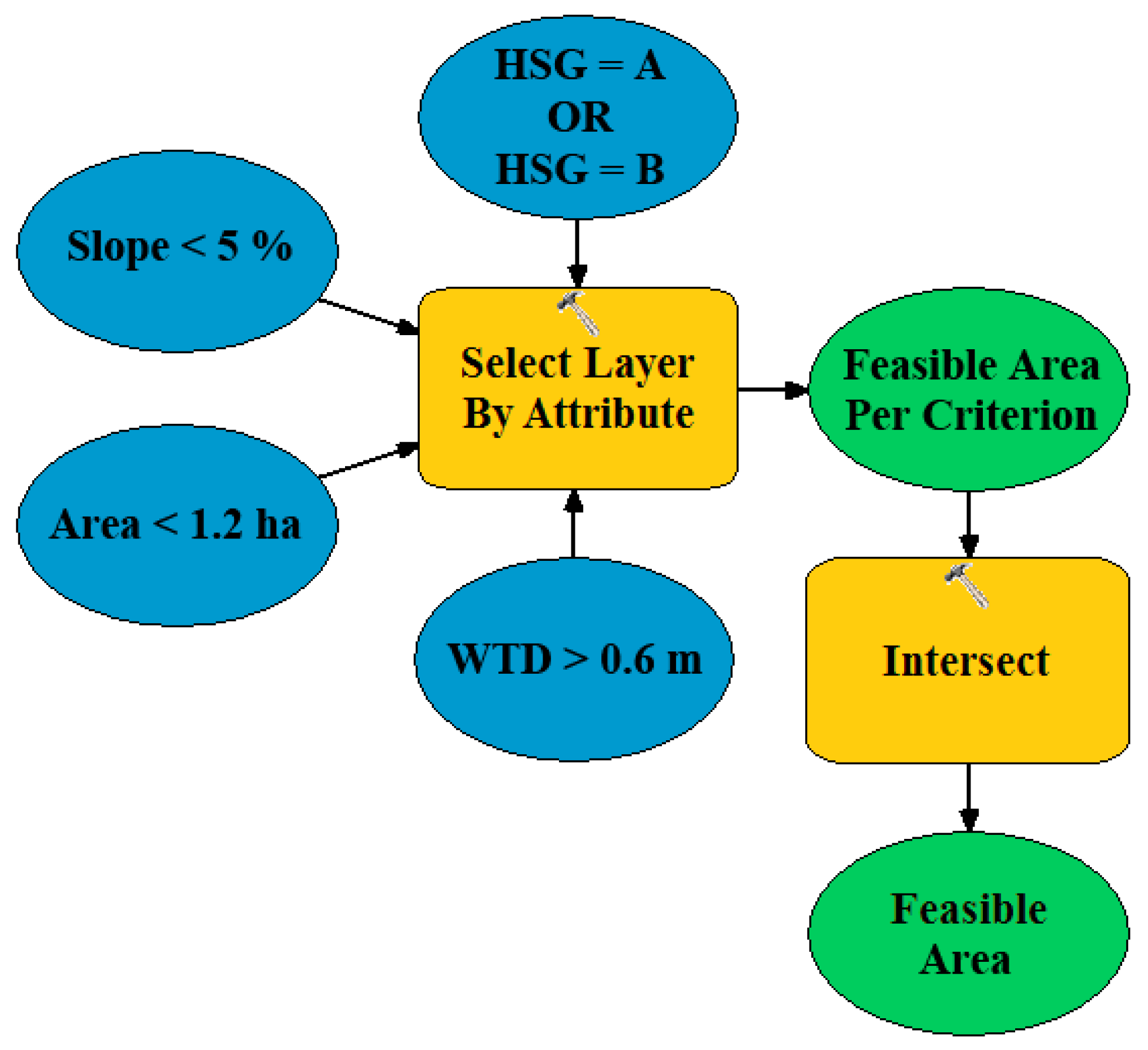
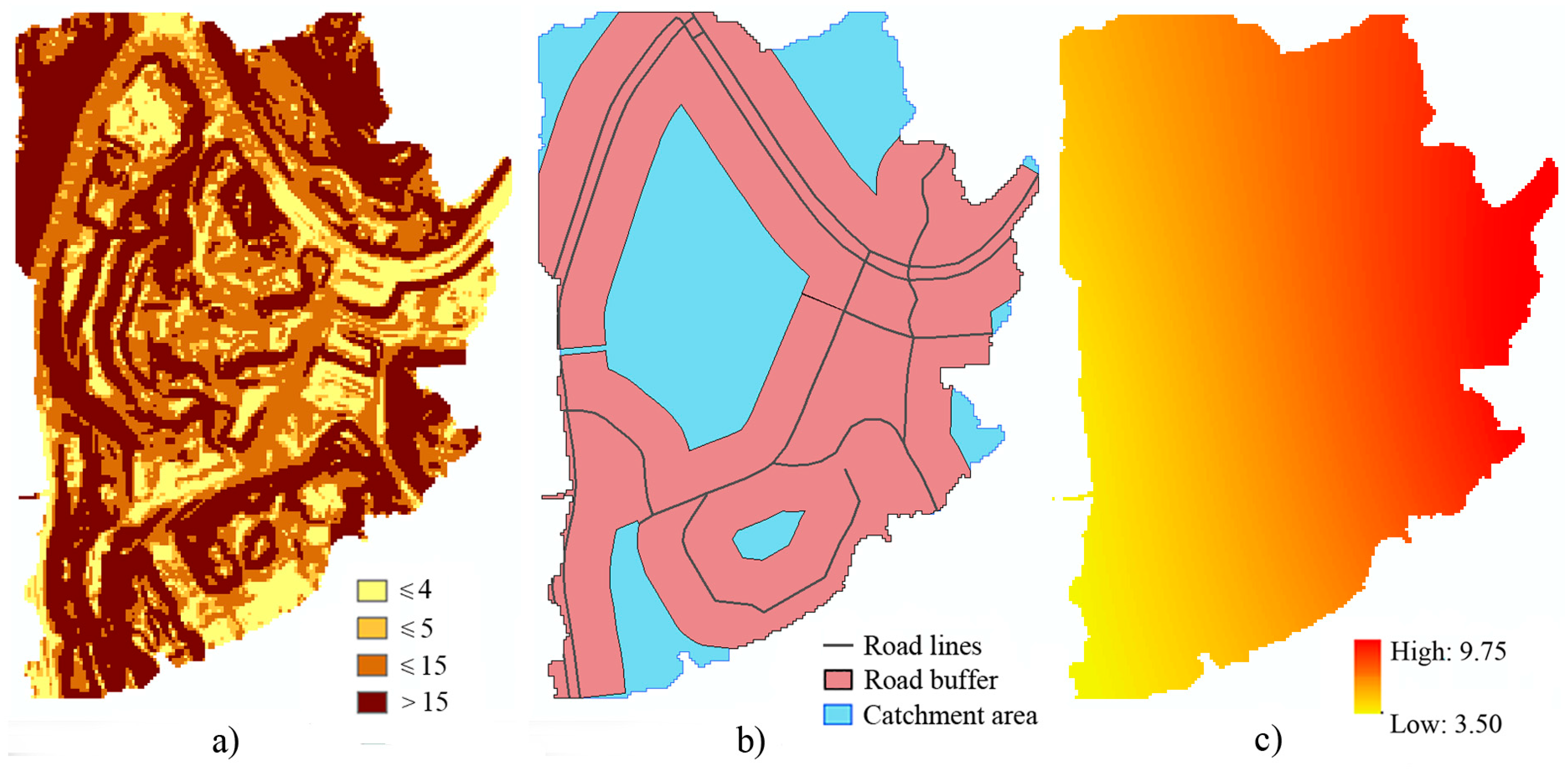
2.1. Search for Feasible Locations for the Implementation of Sustainable Drainage Systems (SuDS)

Table 1 lists the set of geometric and hydrologic criteria to fulfil for the implementation of SuDS in urban catchments. The types of SuDS considered corresponded to those available in the LID Control Editor [24] of SWMM, which is a specific module for the modelling and simulation of these systems. The criteria, which were derived from several reports and manuals related to SuDS [25,26,27,28,29], refer to the recommended maximum drainage area that is considered suitable for each system, the desired Hydrologic Soil Group (HSG) of the underlying layers, the maximum or minimum distances to be kept in relation to buildings, roads and streams, the degree of flatness in the area and the minimum depth to groundwater from the bottom of SuDS.
These feasibility criteria define the set of physical factors that need to be confirmed at site for implementing SuDS. Drainage area indicates the maximum contributing external area that is recommended for each practice, according to their infiltration capability and spatiotemporal relationship to the routing process. The slope restrictions are established according to the same reasons, which delimit the degree of flatness associated with the location of SuDS. HSG stands for the infiltration rate of the soil and relates to the ease of filtering of water through the bottom of the system. Similarly, the depth from the base of the practice to groundwater must be sufficient to allow adequate infiltration. Building buffer is a criterion that only applies to those SuDS that can be installed near these systems and refer to the minimum and maximum recommended distance to ensure that roofshed is properly drained. Bio-retention cells are commonly used as road verges, which justify the existence of the criterion about their proximity to these infrastructures. The last criterion involves that some SuDS must be placed outside the area of influence of streams, in order to minimize the impact on them. These criteria are not exclusive and might be complemented with some others like minimum area in relation to the catchment [30], possible combination with underdrains, traffic loads or type of groundwater reserve.
The intersection of these conditions was accomplished using ModelBuilder [31], which is the visual programming language of ArcGIS to build geoprocessing workflows. The Select Layer By Attribute tool was applied to combine the criteria shown in Table 1 and map the areas where all the conditions required for the implementation of SuDS were met. Figure 1 details this process for the location of PPS. Feasible areas per criterion were added through a cumulative process which stored the zones that fulfilled each of the criteria to be met regarding drainage area, slope, HSG and Water Table Depth (WTD). The operation ended with the application of the Intersect tool, which determined which areas met all the conditions together.
Drainage area is a variable that can be automatically calculated in ArcGIS for any polygon using the Calculate Geometry tool, whilst HSG is a parameter that classifies soil infiltration rate according to four categories set by the Soil Conservation Service (SCS) [32], which can be matched to the geologic map of the study area.
Since the buffer-related criteria are based on keeping a distance with respect to either artificial or natural elements that interact with SuDS, they were all determined according to the same procedure. Regarding buildings and roads, the process simply consisted of using the Buffer tool to enlarge any of the two elements and obtain the area within which SuDS could be implemented. As for streams, an additional step involving the application of the Erase tool was also required to subtract the area obtained through the Buffer from the whole catchment area, in order to determine the spaces that were further than 30 m from the streams.
The identification of feasible areas in terms of slope stemmed from a raster layer with the slope for each cell into which the catchment area was divided, whose values were calculated from a Digital Terrain Model (DTM) through the Slope tool. The Raster Calculator tool allowed the extraction of those areas fulfilling the slope limits to be met, which according to Table 1 were 4%, 5% and 15%.
Water Table Depth is the most complex criterion in terms of characterization, because the source data on which it is based consisted of a grid from global observations of groundwater level. This grid was converted into a continuous surface for further modelling using spatial interpolation techniques, which enabled the prediction of values at unsampled locations in the workspace enclosed by such points. Three deterministic and three geostatistical interpolation methods were used to model this criterion [33]: Inverse Distance Weighting, Radial Basis Functions, Local Polynomial Interpolation, Ordinary Kriging, Simple Kriging and Empirical Bayesian Kriging. The interpolation surfaces determined through their application were evaluated using the coefficient of determination (R2) [34] and the Root-Mean Squared Error (RMSE) [35]. In addition, prior to Kriging, the assumptions of normality and stationarity of the dataset to be interpolated were checked using the Shapiro–Wilk test and a semivariogram cloud.

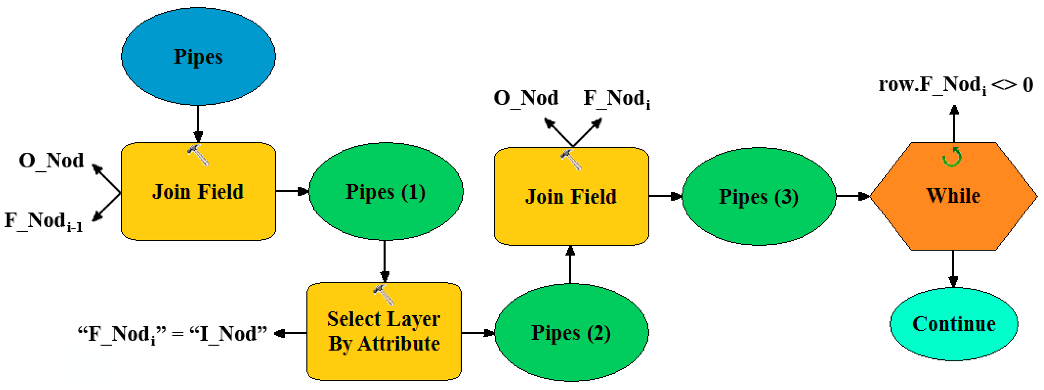
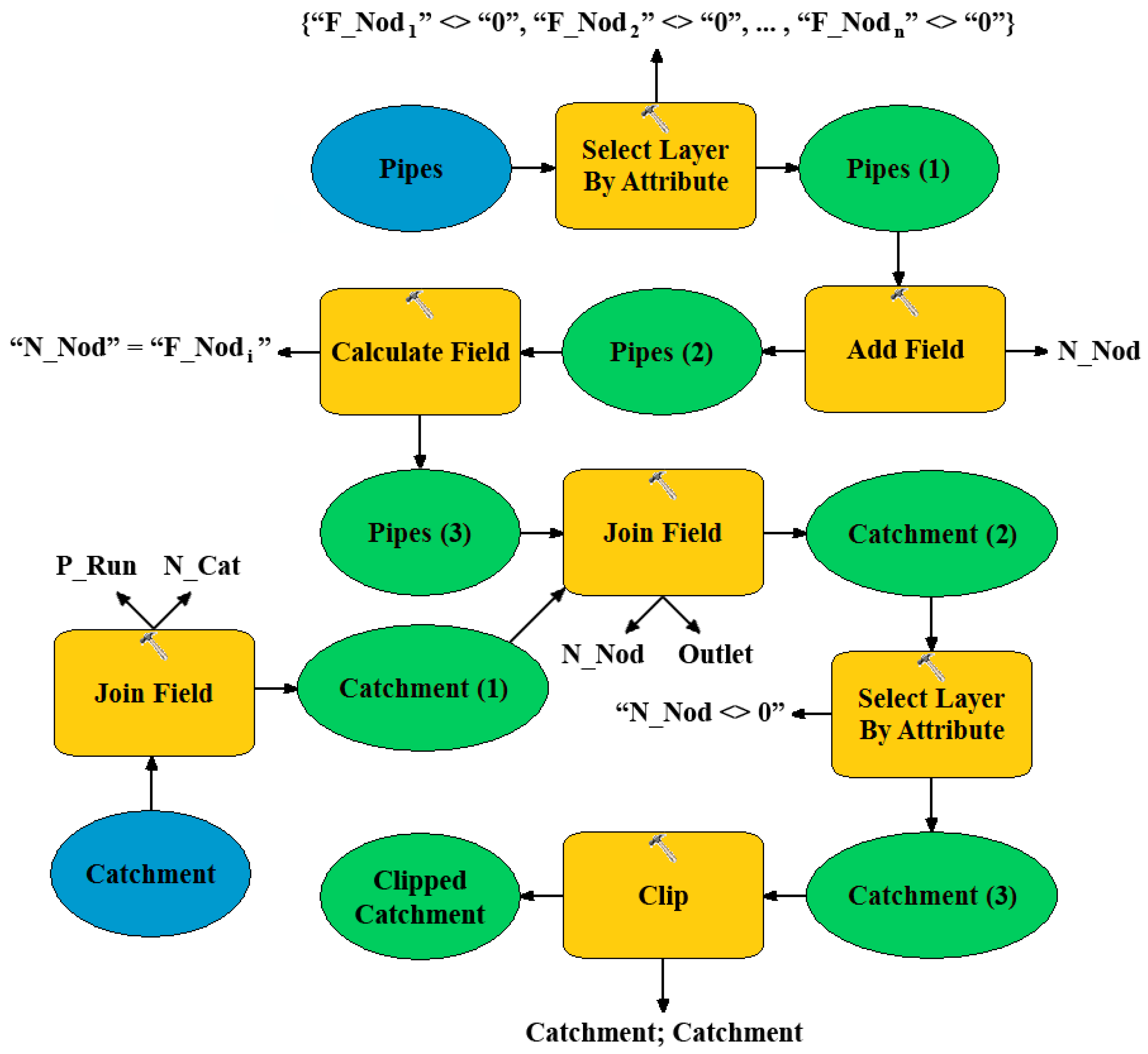
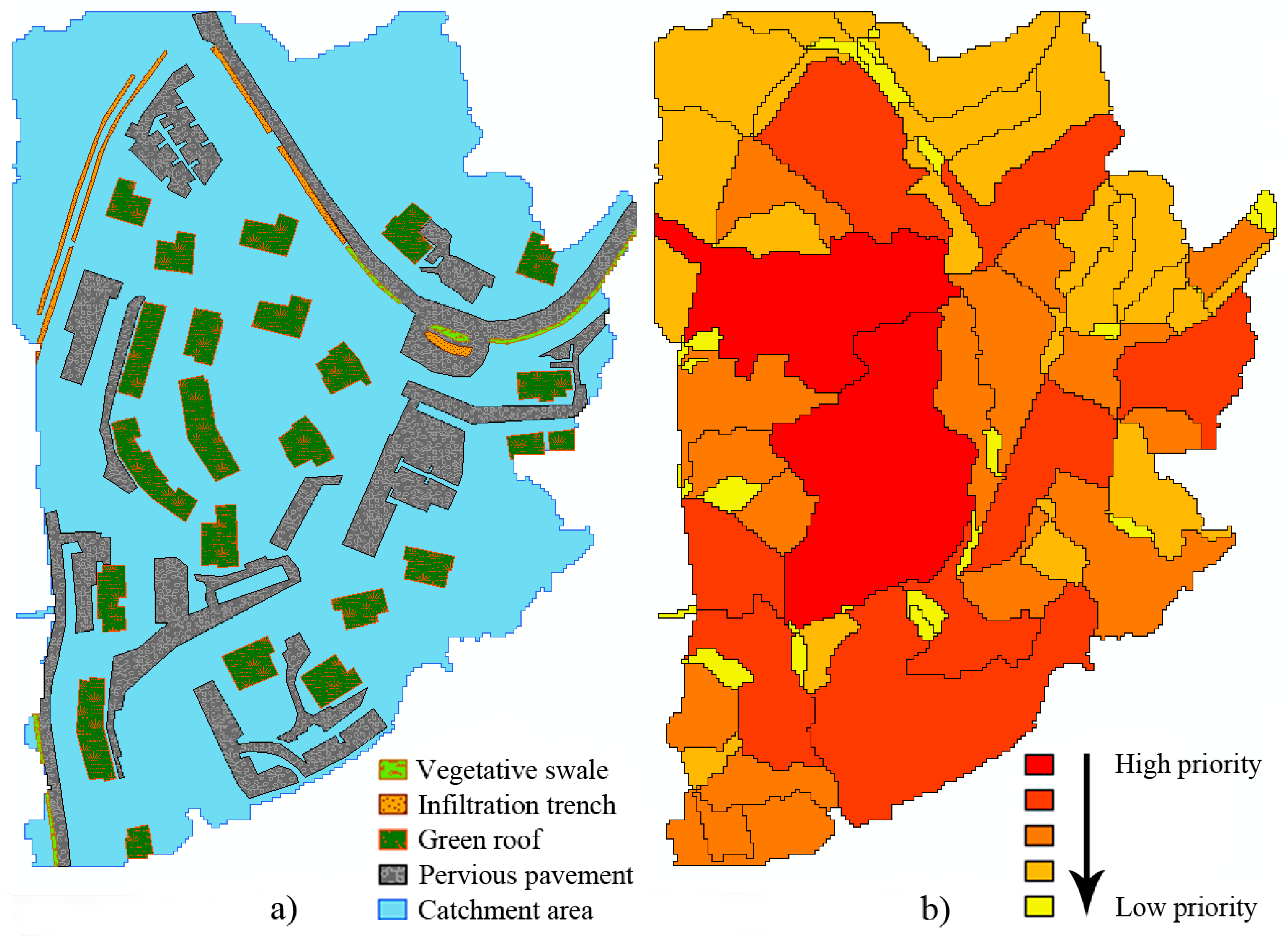
2.2. Prioritization of Flood-Sensitive Areas

This step generated a prioritization map to highlight those areas in the catchment that needed to be retrofitted, according to two main aspects: the set of flooded nodes in the sewer network and peak flow rates in the subcatchments. The inputs required to carry out this task were: (1) a topology containing the initial and final node for each conduit in the sewer network; (2) the list of flooded nodes associated with different rainfall scenarios; and (3) peak runoff rates corresponding to each subcatchment forming the whole catchment area. The first input proceeded from data collection, whilst the two others were results of the stormwater simulations in SWMM. The linkage between SWMM and ArcGIS was achieved through MS Excel [36], a format that allows the results to be imported from SWMM and their subsequent export to ArCGIS.
The sequence of operations for the identification of flood-related nodes is depicted in Figure 2. This algorithm allowed the prioritization to be limited to flood-sensitive areas only through a backward search of those subcatchments flowing directly or indirectly to a flooded node. The process started by matching the column (field in GIS terms) exported to MS Excel with the flooded nodes (“F_Nodi”) identified in SWMM with the outlet nodes (“O_Nod”) of each conduit in the GIS layer “Pipes” using the Join Field tool (“Pipes (1)”). The Select Layer By Attribute tool added the condition that the flooded nodes had to coincide with the conduit input nodes (“I_Nod”), which resulted in “Pipes (2)”. Then, the Join Field tool was applied again to add the nodes preceding the flooded ones (“Pipes (3)”). This process was repeated until the output layer “Pipes (3)” was empty, which meant that the last nodes included in the process had no predecessors. In ModelBuilder terms, this was represented through a While iterator which stopped once all the nodes in the last joined field were equal to 0; i.e., it continued iterating whilst any of the nodes was not 0 (row.F_Nodi <> 0).
All of the nodes that had been stored in the n fields created in the process shown in Figure 2 were associated with the subcatchments that flowed into them as illustrated in Figure 3. As in the previous operation, the Join Field tool was used to append the field “P_Run” with the data on peak runoff from the SWMM results to the field “N_Cat” in the GIS layer of subcatchments (“Catchment”), in order to prioritize them according to their infiltration capability (“Catchment (1)”). The selection of the stored nodes from the layer “Pipes” was carried out using the Select Layer By Attribute tool with the following condition: {F_Nod1 <> 0, F_Nod2 <> 0, …, F_Nodn <> 0} (“Pipes (1)”). The combination of the Add Field (“Pipes (2)”) and Calculate Field (“Pipes (3)”) tools resulted in a new field (“N_Nod”) in the layer, which included the nodes selected in each “F_Nodi” field. This new field was joined to the “Catchment” layer based on its field “Outlet”, in order to identify the subcatchments that flowed directly or indirectly to a flooded node (“Catchment (2)”). The process ended with the application of the Clip tool (“Clipped Catchment”), which extracted such subcatchments from the “Catchment” layer based on the condition previously specified in the Select Layer By Attribute tool (N_Nod <> 0) (“Catchment (3)”).

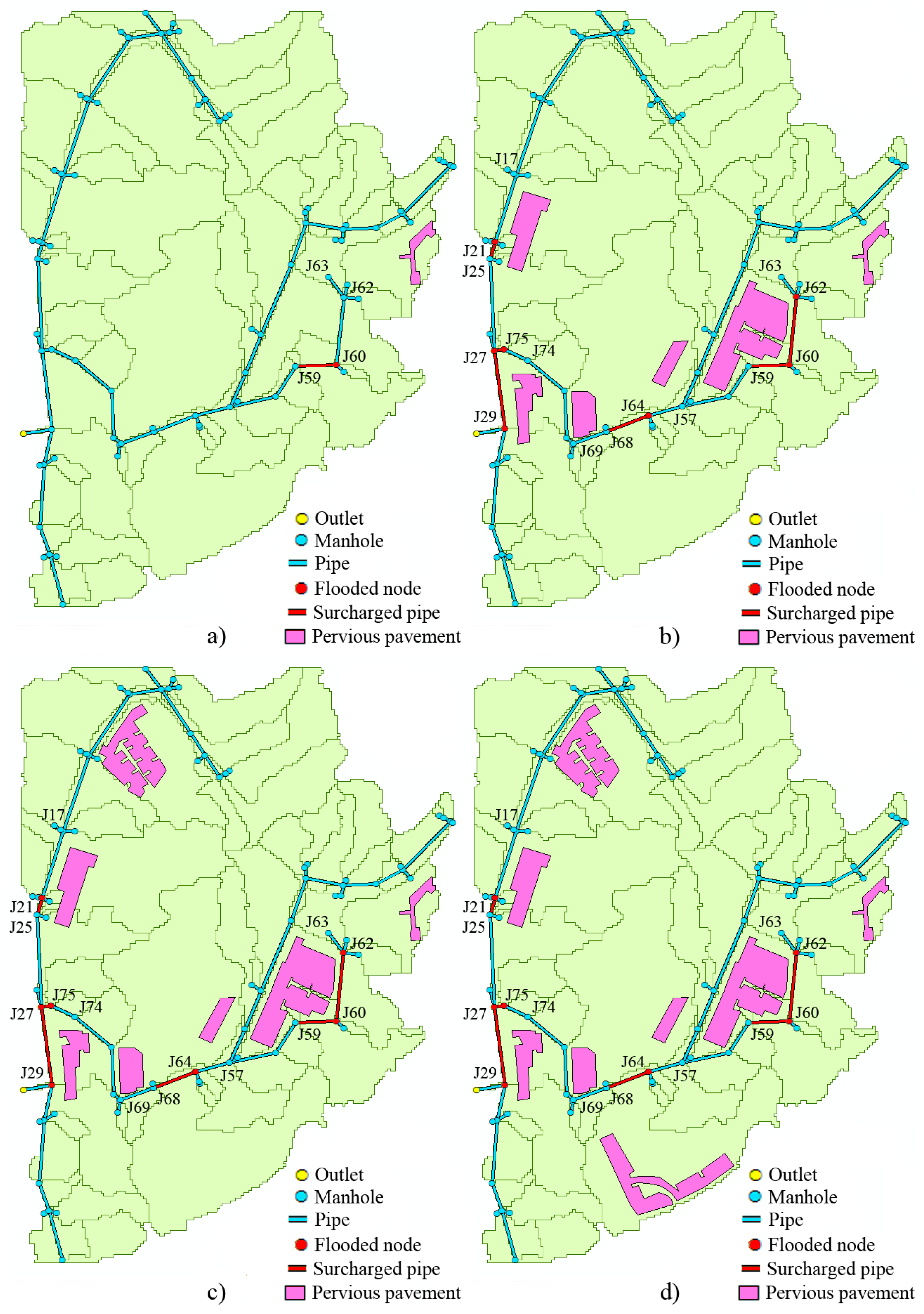
2.3. Hydrological Simulation of Permeable Pavement Systems (PPS)

Once feasible areas to install PPS were identified and prioritized, the urban catchment to be modelled was simulated under its new hydrological configurations with PPS, in order to evaluate the potential impact of the areas covered by these systems on its response. SWMM’s LID Control Editor allowed the eight types of SuDS shown in Table 1 to be modelled by characterizing the layers that form them. In the case of PPS, these layers are the following: surface, pavement, soil (bedding layer) and storage (base).
The values recommended by PPS-related institutes and associations to parameterize these layers [37,38,39,40,41] and previous studies on the use of SWMM to model these systems [23,42] led to define the three cross-sections shown in Table 2, which represent the three major PPS types highlighted by specialized literature sources [25,28,43]: Porous Asphalt (PA), Porous Concrete (PC) and Permeable Interlocking Concrete Pavement (PICP). These cross-sections are representative because institutes and associations specialized in the materials forming the pavement layer suggest them as characteristic. Furthermore, they correspond to the overall engineering properties of each PPS type, whilst the thicknesses of the different layers constituting them were established to result in the same total value (130 mm), in order to enable their direct comparison under the same circumstances.
Manning’s roughness coefficient went from 0.011 for continuous surfaces to 0.030 for PICP [44], in order to represent the extra irregularities involved by discontinuous surfaces. A void ratio of 0.20, 0.25 and 0.10 was set for the pavement layers of PA, PC and PICP, respectively. Thus, the voids of PICP represented 10% of its total area, which resulted in an impervious surface fraction of 0.90. The bedding and base layers consisted of open graded aggregate as suggested in Jato-Espino et al. [45] according to the American Association of State Highway and Transportation Officials (AASHTO) gradation. The base of PICP consisted of a combination of No. 57 and No. 3 stone (150 mm each), which were also the types of aggregate used for the bedding layer (30 mm) and base (300 mm) of PA, respectively. The pavement layer in PC was laid directly onto a 300 mm base of No. 57 stone [40,43]. The porosity of the open-graded materials was set at 0.40, in order to comply with the commonly required minimum value of 0.32 for in-situ aggregate [37].
The clogging capacity of the pavement was not explicitly modelled as a single parameter but included in its permeability capacity. Assuming an initial infiltration rate of 2540 mm/h, PPS are considered to fail when this capacity is less than 254 mm/h [37] (10% of the original value). Based on the mean values provided by the U.S. Geological Service (USGS) for new permeable pavement [46], permeability of the three surfaces under study was reduced according to that ratio to represent their condition at the end of their life, in order to obtain conservative results and conclusions. The fact that these values were obtained from the same source was key in considering them as valid references for comparative purposes. Similarly, permeability of open-graded materials in lower layers was parameterized proportionally to the gradation of the aggregate, according to a range of values between 1270 and 5080 mm/h [37]. Slope is a GIS-based parameter whose values were derived from the calculation of mean slope in the areas covered by each PPS type.
The impact of the cross-sections represented in Table 2 on the hydrological response of urban catchments was evaluated through inferential statistical analyses. Tests belonging to this branch of statistics are usually applied to reject the null hypothesis in favour of the alternative hypothesis, which is expected to be the cause of the phenomenon under analysis. This was determined through the p-value, which indicates the probability of wrongly rejecting the null hypothesis if it is true. If the p-value is below the significance level, the probability of error is lower than α [47], which was set at 0.05 [48].
Normality of the data forming the hydrographs obtained for the three types of PPS determined whether parametric or non-parametric tests had to be applied. The Shapiro–Wilk test [49], which has been proved to be more reliable to check normality than other widely used tests such as Kolmogorov–Smirnov or Lilliefors [50], was chosen for examining normality. Based on these results, the existence of statistically significant differences between the hydrographs associated with different PPS-related scenarios was assessed using the following tests: Analysis of Variance (ANOVA) [51] or Kruskal–Wallis [52] for three or more samples (PA, PC and PICP) and Student’s t [53] or Mann–Whitney U [54] for two samples (without PPS and with PPS).

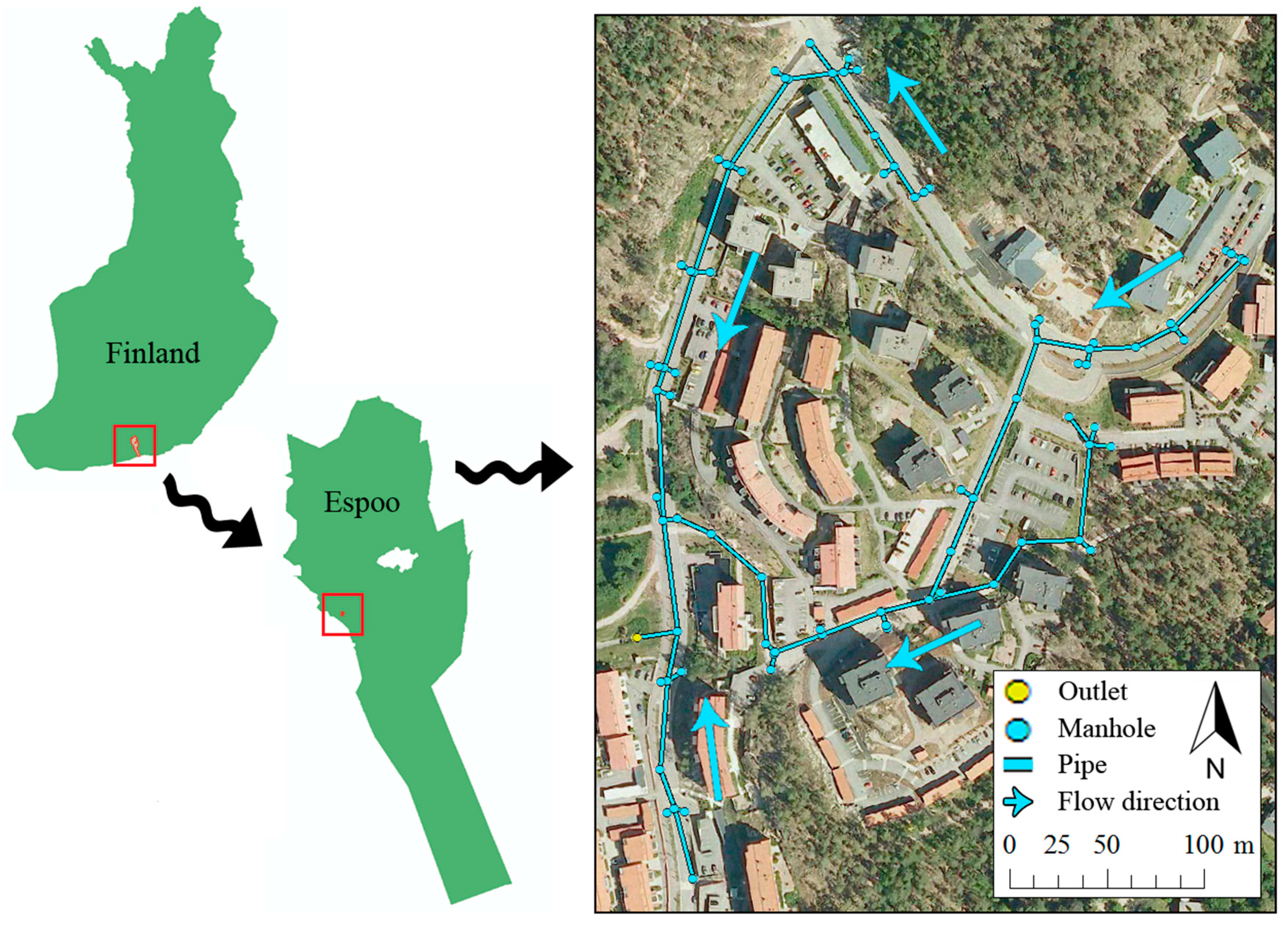
3. Results and Discussion: A Case Study in Espoo, Finland

The results of this research were generated from the application of the proposed methodology to a case study consisting of a real urban catchment located in Espoo, southern Finland. The study catchment experienced rapid development and transitioned from being a coniferous forest in 2001 to a residential area in 2006 [55]. Figure 4 shows the location of the catchment and the spatial distribution of its sewer network, which was provided by the Helsinki Region Environmental Services Authority HSY.
Figure 4 also depicts the aerial photography of the study catchment in 2007 [56], when it was at full development. A Digital Terrain Model (DTM) with a cell size of 2 m was acquired from the National Land Survey of Finland [57], whilst the Geological Survey of Finland revealed that the study catchment laid on a layer of sandy till with bedrock below it [23], which most likely corresponds to a HSG of B. A set of 60 points with values of Water Table Depth near the catchment area was extracted from the global grid created by Fan et al. [58] at 1,603,781 sites worldwide from government archives and published literature.
The study catchment was delineated and simulated in SWMM by Jato-Espino et al. [59], who determined that it was formed of 79 subcatchments covering 10.535 ha and optimized its stormwater modelling using Design of Experiments (DOE) with three monitored calibration (CAL 1, CAL 2 and CAL 3) and validation (VAL 1, VAL 2 and VAL 3) rainfall events (see Table 3). The calibration of the simulations revealed that six parameters had a statistically significant impact on the discharge of the study catchment. Below are specified the calibrated values for each of them, whose combination maximized the fit between observed and predicted outflow: percentage of imperviousness (80% of the initial value obtained using GIS tools), width (80.4% of the initial value obtained using GIS tools), slope (115.15% of the initial value obtained using GIS tools), Manning’s roughness for impervious area (0.0135), Depth of depression storage on impervious areas (0.379 mm) and Manning’s roughness for conduits (0.015). The simulation of the validation events with these calibrated parameters reproduced the real hydrographs monitored at the outlet of the catchment with high accuracy, as demonstrated by the goodness-of-fit measures used to test them (see Table 3): Root-Sum Squared Error (RSSE), coefficient of determination (R2) and Nash–Sutcliffe model efficiency coefficient (E).
Once the accuracy of the model was validated, the study catchment was re-simulated with the calibrated parameters by these same authors using synthetic storms designed for different return periods and climate scenarios [59], in order to assess its response to storm events caused by Climate Change. Hence, in addition to the stationary scenario in which precipitation was assumed to remain constant over time, two different greenhouse gas concentration trajectories were considered: RCP4.5 and RCP8.5 [60]. Table 4 lists the values of Annual Maximum Daily Precipitation (AMDP) associated with each combination of return period and climate scenario. These values of AMDP were used to design synthetic storms through the combination of Intensity–Duration–Frequency (IDF) curves and the Alternating Block Method. Their duration was 106 min in all cases, according to the lag time of the total catchment. These data were used as the basis for carrying out the prioritization of flood-sensitive areas in the study catchment.

3.1. Search for Feasible Locations for the Implementation of Sustainable Drainage Systems (SuDS)

The search for feasible locations for the implementation of SuDS in the study catchment started with the preparation of maps related to the geometric and hydrologic criteria to be met by each system according to Table 1: HSG, slope, building buffer, road buffer, stream buffer, Water Table Depth and area. Since the hydrological condition of the soil below the study catchment corresponded to an HSG of B, there was no restriction in these terms for any type of SuDS, which required at most a type B soil.
Slope in the catchment area was determined from the DTM and classified according to the three thresholds defined in Table 1: 4%, 5% and 15% (see Figure 5a). The area corresponding to these thresholds covered 14.40%, 20.78% and 55.49% of the whole study catchment, which provided multiple opportunities to install different types of SuDS. Since the location of the downspouts in the buildings was unknown and there was no stream close enough (<30 m) to the study catchment to be considered, the buffer-related calculations were limited to roads (see Figure 5b), whose presence only restricted the implementation of bio-retention cells (see Table 1). In this case, the ratio of road buffer areas to the whole catchment area was 70.91%.
An exploratory analysis of the dataset with values of Water Table Depth was carried out in the first place to model this criterion. Normality of this dataset was ensured by the p-value reached according to the Shapiro–Wilk test (0.092), whilst the shape of the semivariogram cloud suggested that there was no spatial autocorrelation between measurements, since the average squared difference of values for all pairs of points increased as the distance between the pairs of points increased. The best combination of coefficient of determination and R2 and Root-Mean Squared Error (RMSE) was provided by Ordinary Kriging, which yielded values of 0.797 and 3.482, respectively. The interpolation surface obtained shown in Figure 5c using this method demonstrated that Water Table Depth was not an issue, since the groundwater level was at least 3.50 m below the ground (see Table 1). The last criterion to check was the maximum area to be covered by SuDS. The combination of feasible zones according to the four other criteria (HSG, buffers, slope and Water Table Depth) demonstrated that no limit in terms of surface area was exceeded.
The intersection of areas in which these criteria were met separately resulted in Figure 6a. Bio-retention cells, which shared locations with either vegetative swales or infiltration trenches, were not included in the map because their area was smaller than that corresponding to any other option. The two remaining types of SuDS listed in Table 1, rain barrels and rooftop disconnection, were not considered either because the location of the downspouts was unknown. This is a refined map, excluding marginal and disconnected feasible areas whose consideration was irrelevant in practical terms. As for overlap, the area associated with vegetative swales in Figure 6a was also valid for infiltration trenches. PPS were the type of SuDS that involved larger feasible area, covering 16.62% of the study catchment, followed by green roofs and infiltration trenches with 9.82% and 1.44%, respectively. This fact, which was consistent with the wide applicability of PPS introduced in previous sections, supported the focus of the methodology on this specific system from now on.

3.2. Prioritization of Flood-Sensitive Areas

Data imported from the stormwater simulations run in SWMM to ArcGIS and the subsequent application of the iterative algorithms summarized in Figure 2 and Figure 3 resulted in the priority map shown in Figure 6b. Although the values of peak runoff obtained in SWMM varied depending on climate scenario and return period, the priority order was constant in all cases and, as expected, was mainly given by the size of subcatchments. It was the only factor having a statistically significant correlation to peak runoff (Pearson’s correlation coefficient of 0.906 with a p-value of 0.000).
This priority map demonstrated that all subcatchments flowed directly or indirectly to a flooded node, due to the geometric arrangement and connectivity of the sewer system in the study catchment. A recent study developed by Jato-Espino et al. [61] demonstrated that this does not necessarily have to be the case, but the number of subcatchments associated with flooded nodes depends on the specifics of the drainage network.

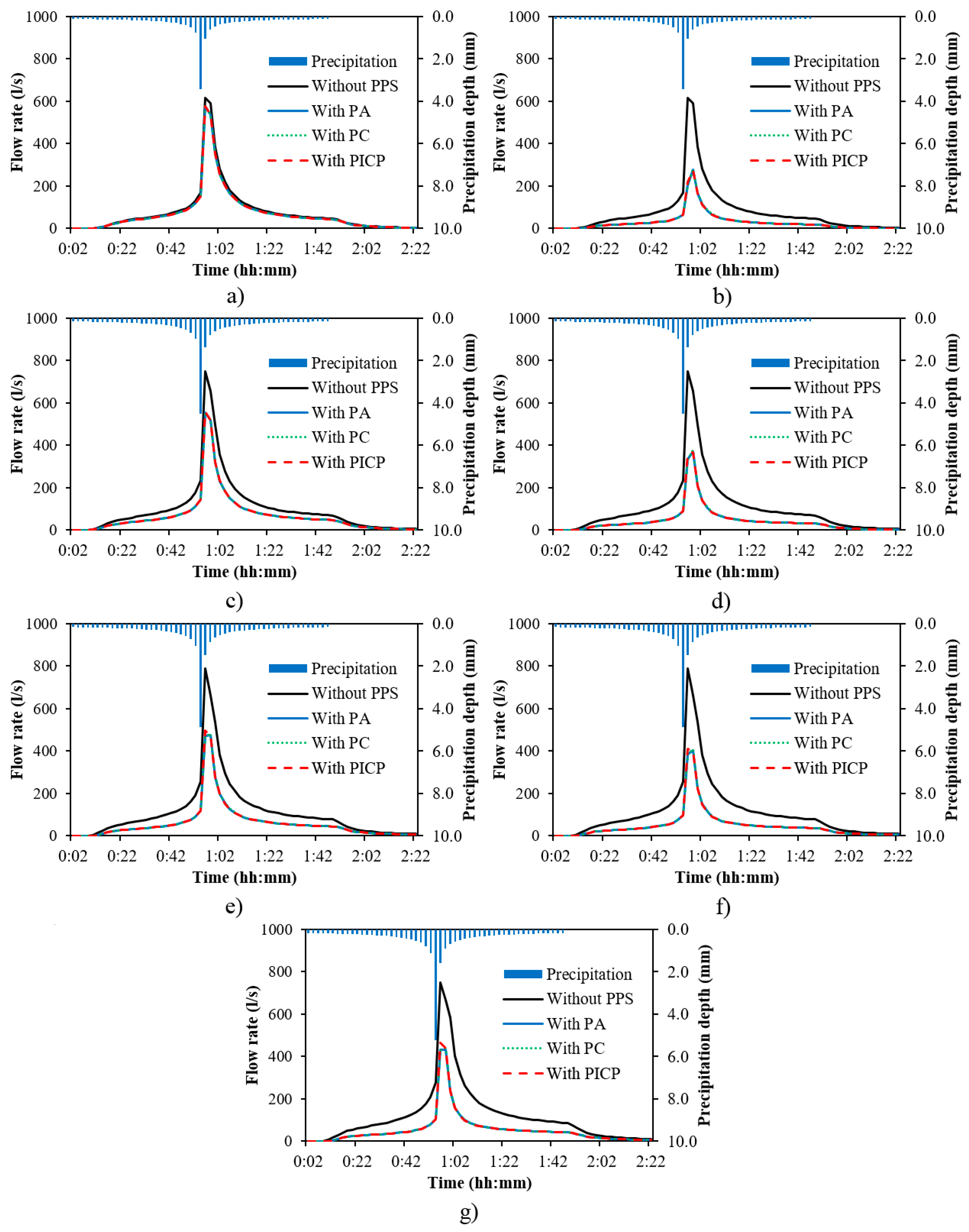
3.3. Hydrological Simulation of Permeable Pavement Systems (PPS)

The information contained in Figure 6 was used to model the influence of PPS on the hydrological response of the study catchment. Firstly, the catchment was simulated without PPS, in order to identify which areas were more sensitive to flooding under the return periods and climate scenarios listed in Table 4. Simulation duration was set at 150 min, since this value proved to be enough for runoff to cease. The time step for reporting was 2 min, in order to match the frequency with which flow rate was originally monitored in the study catchment [59], whereas routing was set at 3 s to minimize surface runoff and flow routing continuity errors. The results yielded by these simulations were then used for locating PPS in strategic areas to avoid node flooding and conduit surcharge along the sewer network. Figure 7 is a representation of the minimum area of PPS required to avoid flooding under different combinations of climate scenario and return period. The location of PPS was limited to parking areas exclusively, in order to reproduce the most feasible and easiest to integrate solutions in practical terms. Therefore, no isolated and/or difficult to connect pavement reach was considered in subsequent calculations.
The simulations proved that the storms associated with a return period of two years were enough to produce floods in the study catchment for the RCP scenarios. In contrast, a value of 10 years was required to cause the same impact under the stationarity assumption, which highlights the increase in drainage capability required by Climate Change. The inclusion of different PPS configurations was found to avoid any flooding problem up to the following return periods: 2, 10 and 50 years for RCP8.5, RCP4.5 and stationary scenarios, respectively. These figures demonstrate the capability of this type of SuDS to mitigate the effects of heavy rainfall events beyond the common magnitudes used to design urban drainage systems (stationary scenarios with return periods of 2, 5 or at most 10 years). In quantitative terms, the presence of PPS involved an average volume reduction at the outlet of the study catchment of 40%–50%.
The stormwater simulation of the catchment configurations illustrated in Figure 7 resulted in the hydrographs represented in Figure 8. Each plot includes the four following hydrographs: without PPS, with Porous Asphalt (PA), with Porous Concrete (PC) and with Permeable Interlocking Concrete Pavement (PICP). Figure 8a,c,e was obtained from the simulation of minimum PPS areas required to avoid flooding, whereas Figure 8b,d,f corresponds to the location of PPS in all available parking areas (see Figure 7d). The comparison of minimum (Min) and maximum (All) PPS areas was introduced to demonstrate the capability of these systems to not only reduce runoff volumes, but also delay peak flows. Figure 8g does not include this distinction, because the minimum and maximum coincided for the mitigation of the 50-year storm in the stationary scenario. As for the combination of RCP4.5 and a return period of 10 years, the minimum PPS area used to avoid flooding was enough to produce a delay in peak flow (see Figure 8e), because only the parking area in the south of the catchment was omitted in comparison with the scheme depicted in Figure 7d.
These hydrographs were analysed using statistical techniques to verify that the hydrological impact of PPS was significant. The p-value obtained for the four hydrographs (without PPS, with PA, with PC and with PICP) for the three return periods (2, 10 and 50 years) and climate scenarios (stationary, RCP4.5 and RCP8.5) using the Shapiro–Wilk test was 0.000 for all these combinations, which suggested that the samples under analysis were not normally distributed and had to be evaluated through non-parametric tests. Hence, the Kruskal–Wallis test was applied to confirm the absence of differences in the hydrographs associated with the PPS types. The p-values, which were 1.000 in all cases, enabled the acceptance of this hypothesis. These results showed that any of the three different types of PPS could be used to compare the results obtained with and without them installed, which demonstrated that the hydrological impact of these systems at a catchment scale was extremely similar. Under these circumstances, the Mann–Whitney U test proved that the differences in hydrological response of the catchment with and without PPS (PA, PC or PICP) were statistically significant in all cases (p-values < 0.05), except for the situation represented in Figure 7a, which involved the inclusion of a PPS area of only 0.031 ha in the east of the study catchment. In overall terms, these results proved that PPS can make a significant difference to the amount of excess stormwater generated in an urban catchment due to intense rainfall events.

4. Conclusions

This research presented and applied a coupled GIS and stormwater modelling framework to prioritize suitable locations for the installation of PPS and simulate their hydrological impact in urban catchments, in order to evaluate their potential to mitigate peak discharge in flood-sensitive areas. The results demonstrated that the hydrological impact of PPS can be maximized if their location is prioritized according to the drainage capacity of urban catchments using spatial site selection tools to identify areas requiring primary action. This inference led to a series of more specific conclusions to be drawn, as listed below:
  • The percentage of feasible area available in the study catchment for the location of SuDS indicated that PPS were the easiest systems to implement in urban areas due to their multifunctionality.
  • The magnitude of lateral inflows in the study catchment was mainly given by the area of its subcatchments, which was the only factor that proved to have a statistically significant correlation to peak runoff rates.
  • The inclusion of PPS was found to reduce runoff volumes and delay hydrograph peaks produced by severe storms beyond the standard return periods (2, 5 and 10 years under stationarity) used to design urban drainage systems.
  • Although the parameters that characterized their layers were different, the differences between the hydrological impacts of the three main PPS cross-sections (PA, PC and PICP) at the scale of the study catchment were negligible.
  • PPS had a statistically significant hydrological impact on the response of the study catchment and reduced discharge by 50% in comparison with situations exclusively based on conventional drainage systems.
The automation of the proposed site selection methodology and the evaluation of the accuracy of stormwater models to characterize PPS through comparison with laboratory tests were identified as the future course of action to continue this research, in order to promote the use of spatial hydrologic tools and validate their reliability.

Acknowledgments

This paper was possible thanks to the research projects RHIVU (Ref. BIA2012-32463), SUPRIS-SUReS (Ref. BIA2015-65240-C2-1-R MINECO/FEDER, UE) and SUPRIS-SUPeI (Ref. BIA2015-65240-C2-2-R MINECO/FEDER, UE), financed by the Spanish Ministry of Economy and Competitiveness with funds from the State General Budget (PGE) and the European Regional Development Fund (ERDF). The authors wish to express their gratitude to all the entities that provided the data necessary to develop this research: Helsinki Region Environmental Services Authority HSY, Map Service of Espoo, National Land Survey of Finland, Geological Survey of Finland, EURO-CORDEX and European Climate Assessment & Dataset.

Author Contributions

Daniel Jato-Espino conceived the research; Nora Sillanpää produced the data required to apply the methodology to the case study; Daniel Jato-Espino and Ignacio Andrés-Doménech carried out the characterization of permeable pavements; Daniel Jato-Espino designed the site selection system and conducted the stormwater simulations; Daniel Jato-Espino, Nora Sillanpää, Susanne M. Charlesworth and Ignacio Andrés-Doménech discussed the results; and Daniel Jato-Espino and Susanne M. Charlesworth wrote the paper.

Conflicts of Interest

The authors declare no conflict of interest. The founding sponsors had no role in the design of the study; in the collection, analyses, or interpretation of data; in the writing of the manuscript, and in the decision to publish the results.

References

  1. Franczyk, J.; Chang, H. The effects of climate change and urbanization on the runoff of the rock creek basin in the Portland Metropolitan Area, Oregon, USA. Hydrol. Process. 2009, 23, 805–815. [Google Scholar] [CrossRef]
  2. Charlesworth, S.M. A review of the adaptation and mitigation of global climate change using sustainable drainage in cities. J. Water Clim. Chang. 2010, 1, 165–180. [Google Scholar] [CrossRef]
  3. Pratt, C.J.; Wilson, S.; Cooper, P. Source Control Using Constructed Pervious Pavements. Hydraulic, Structural and Water Quality Performance Issues; CIRIA: London, UK, 2002. [Google Scholar]
  4. Rodriguez-Hernandez, J. Estudio, Análisis y Diseño de Secciones Permeables de Firmes Para Vías Urbanas con un Comportamiento Adecuado Frente a la Colmatación y con la Capacidad Portante Necesaria para Soportar Tráficos Ligeros. Ph.D. Thesis, Universidad de Cantabria, Santander, Spain, 2008. [Google Scholar]
  5. Hollinrake, P.G. Permeable Pavements; Report SR 264; HR Wallingford: Wallingford, UK, 1991; pp. 1–58. [Google Scholar]
  6. Jato-Espino, D.; Charlesworth, S.M.; Bayon, J.R.; Warwick, F. Rainfall-runoff simulations to assess the potential of SuDS for mitigating flooding in highly urbanized catchments. Int. J. Environ. Res. Public Health 2016, 13. [Google Scholar] [CrossRef] [PubMed]
  7. Perez-Pedini, C.; Limbrunner, J.F.; Vogel, R.M. Optimal location of infiltration-based best management practices for storm water management. J. Water Resour. Plan. Manag. 2005, 131, 441–448. [Google Scholar] [CrossRef]
  8. Cooper, D.; Calvert, J. Draft Strategic Flood Risk Assessment; Ipswich Borough Council: Ipswich, UK, 2007; p. 77.
  9. Kodz, M.; Caroline Mills, C. Sustainable Drainage Systems for Local Development Framework; Halcrow Group Limited: London, UK, 2011; p. 44. [Google Scholar]
  10. Doncaster, S.; Stovin, V.; Brian Morrow, B. Lower Irwell Valley, Salford integrated urban drainage pilot project. Integr. Urban Drain. Pilot. 2008, TRE344, 3–30. [Google Scholar]
  11. Dearden, R.A.; Price, S.J. A proposed decision-making framework for a national infiltration SuDS map. Manag. Environ. Qual. Int. J. 2012, 23, 478–485. [Google Scholar] [CrossRef] [Green Version]
  12. Becker, M.; Geretshauser, G.; Spengler, B.; Sieker, H. A stormwater management information system for the catchment area of the River Emscher. Water Pract. Technol. 2006, 1, 1–8. [Google Scholar] [CrossRef]
  13. Sieker, H.; Bandermann, S.; Becker, M.; Raasch, U. Urban stormwater management demonstration projects in the Emscher Region. In First SWITCH Scientific Meeting; The SWITCH Consortium: Birmingham, UK, 2006; pp. 1–8. [Google Scholar]
  14. Moore, S.L.; Stovin, V.R.; Wall, M.; Ashley, R.M. A GIS-based methodology for selecting stormwater disconnection opportunities. Water Sci. Technol. 2012, 66, 275–283. [Google Scholar] [CrossRef] [PubMed]
  15. Shoemaker, L.; Riverson, J., Jr.; Alvi, K.; Zhen, J.X.; Paul, S.; Rafi, T. SUSTAIN—A Framework for Placement of Best Management Practices in Urban Watersheds to Protect Water Quality; EPA/600/R-09/095; U.S. Environmental Protection Agency: Washington, DC, USA, 2009; pp. 1–202.
  16. Charlesworth, S.M.; Warwick, F.; Lashford, C. Decision-making and sustainable drainage: Design and scale. Sustainability 2016, 8, 782. [Google Scholar] [CrossRef]
  17. Viavattene, C.; Scholes, L.; Revitt, D.M.; Ellis, J.B. A GIS based decision support system for the implementation of stormwater best management practices. In Proceedings of the 11th International Conference on Urban Drainage, Scotland, UK, 31 August–5 September 2008; Volume 11, pp. 1–9.
  18. Ellis, J.B.; Viavattene, C.; Chlebek, J.; Hetherington, D. Integrated modelling for urban surface water exceedance flows. Proc. Inst. Civ. Eng. Struct. Build. 2012, 165, 543–552. [Google Scholar] [CrossRef]
  19. Environmental Systems Research Institute (ESRI). ArcGIS for Desktop; ESRI: Redlands, CA, USA, 2013. [Google Scholar]
  20. United States Environmental Protection Agency (U.S. EPA). SWMM 5.1.010; U.S. EPA: Washington, DC, USA, 2015.
  21. Temprano, J.; Arango, Ó.; Cagiao, J.; Suárez, J.; Tejero, I. Stormwater quality calibration by SWMM: A case study in Northern Spain. Water SA 2006, 32, 55–63. [Google Scholar] [CrossRef]
  22. Beling, F.A.; Garcia, J.I.B.; Paiva, E.M.C.D.; Bastos, G.A.P.; Paiva, J.B.D. Analysis of the SWMM model parameters for runoff evaluation in Periurban Basins from Southern Brazil. In Proceedings of the 12th International Conference on Urban Drainage, Porto Alegre, Brazil, 11–16 September 2011; pp. 1–8.
  23. Guan, M.; Sillanpää, N.; Koivusalo, H. Modelling and assessment of hydrological changes in a developing urban catchment. Hydrol. Process. 2015, 29, 2880–2894. [Google Scholar] [CrossRef]
  24. Rossman, L. Storm Water Management Model User’s Manual—Version 5.0; U.S. Environmental Protection Agency: Cincinnati, OH, USA, 2010.
  25. Woods-Ballard, B.; Wilson, S.; Udale-Clarke, H.; Illman, S.; Scott, T.; Ashley, R.; Kellagher, R. The SuDS Manual; CIRIA: London, UK, 2015; p. 937. [Google Scholar]
  26. Clar, M.L.; Barfield, B.J.; O’Connor, T.P. Section 5: BMP Types and Selection. In Stormwater Best Management Practice Design Guide; EPA/600/R-04/121; United States Environmental Protection Agency (U.S. EPA): Washington, DC, USA, 2004; pp. 71–88. [Google Scholar]
  27. Muthukrishnan, S.; Selvakumar, A. Chapter 3: Structural BMP Design Practices. In The Use of Best Management Practices (BMPs) in Urban Watersheds; EPA/600/R-04/184; United States Environmental Protection Agency (U.S. EPA): Washington, DC, USA, 2004; pp. 78–170. [Google Scholar]
  28. Beaupre, D.; Jencks, R.; Minick, S.; Mundy, J.; Navarret, A. Appendix A: BMP Fact Sheets. In San Francisco Stormwater Design Guidelines; San Francisco Public Utilities Commission: San Francisco, CA, USA, 2010; pp. 24–31. [Google Scholar]
  29. Sample, D.J. Best management practice fact sheet 1: Rooftop disconnection. Va. Coop. Ext. 2013, 426–120, 2–3. [Google Scholar]
  30. Bratieres, K.; Fletcher, T.D.; Deletic, A.; Zinger, Y. Nutrient and sediment removal by stormwater biofilters: A large-scale design optimisation study. Water Res. 2008, 42, 3930–3940. [Google Scholar] [CrossRef] [PubMed]
  31. ArcGIS for Desktop. ModelBuilder—Creating Tools Tutorial. Available online: http://desktop.arcgis.com/es/arcmap/10.3/analyze/modelbuilder/what-is-modelbuilder.htm (accessed on 23 March 2016).
  32. Cronshey, R.; McCuen, R.H.; Miller, N.; Rawls, R.; Robbins, S.; Woodward, D. Urban Hydrology for Small Watersheds; TR-55; U.S. Department of Agriculture (USDA): Washington, DC, USA, 1986; pp. 13–21.
  33. Childs, C. Interpolating Surfaces in ArcGIS Spatial Analyst; ArcUser: Redlands, CA, USA, 2004. [Google Scholar]
  34. Hirsch, R.M.; Helsel, D.R.; Cohn, T.A.; Gilroy, E.J. Statistical analysis of hydrologic data. In Handbook of Hydrology; Maidment, D.R., Ed.; McGraw-Hill: New York, NY, USA, 1993; pp. 1–55. [Google Scholar]
  35. Chai, T.; Draxler, R.R. Root Mean Square Error (RMSE) or Mean Absolute Error (MAE)?—Arguments against avoiding RMSE in the literature. Geosci. Model Dev. 2014, 7, 1247–1250. [Google Scholar] [CrossRef]
  36. Microsoft Office. MS Excel 2013; Microsoft Corporation: Redmond, WA, USA, 2013. [Google Scholar]
  37. Smith, D.R. Permeable Interlocking Concrete Pavements, 3rd ed.; Interlocking Concrete Pavement Institute: Burlington, ON, Canada, 2006. [Google Scholar]
  38. National Asphalt Pavement Association (NAPA). Porous Asphalt Pavements for Stormwater Management. Design, Construction and Maintenance Guide; National Asphalt Pavement Association: Lanham, MD, USA, 2008. [Google Scholar]
  39. Interlocking Concrete Pavement Institute (ICPI). A Comparison Guide to Porous Asphalt and Pervious Concrete; Interlocking Concrete Pavement Institute: Chantilly, VA, USA, 2009. [Google Scholar]
  40. ACI Committee 522. Specification for Pervious Concrete Pavement; American Concrete Institute: Farmington Hills, MI, USA, 2013. [Google Scholar]
  41. Federal Highway Administration (FHWA). Permeable Interlocking Concrete Pavement; HIF-15-007; Federal Highway Administration: Washington, DC, USA, 2015; pp. 3–4.
  42. Zhang, S.; Guo, Y. SWMM simulation of the storm water volume control performance of permeable pavement systems. J. Hydrol. Eng. 2015, 20. [Google Scholar] [CrossRef]
  43. Tennessee Department of Environment and Conservation (TDEC). Permeable Pavement. In Tennessee Permanent Stormwater Management and Design Guidance Manual; University of Tennessee: Knoxville, TN, USA, 2014; pp. 187–214. [Google Scholar]
  44. McCuen, R.H.; Johnson, P.; Ragan, R. Highway Hydrology: Hydraulic Design Series, 2nd ed.; Federal Highway Administration: Washington, DC, USA, 1996. [Google Scholar]
  45. Jato-Espino, D.; Rodriguez-Hernandez, J.; Andrés-Valeri, V.C.; Ballester-Muñoz, F. A Fuzzy Stochastic Multi-Criteria Model for the Selection of Urban Pervious Pavements. Expert Syst. Appl. 2014, 41, 6807–6817. [Google Scholar] [CrossRef]
  46. Bannerman, R.; Horwatich, J.; Selbig, B. Technical Note for Conducting Pavement Surface Infiltration Rate, Pollutant Load and Runoff Volume Reduction Modeling in Accordance with WDNR Conservation Practice Standard 1008, Permeable Pavement; United States Geological Survey (USGS): Reston, VA, USA, 2014.
  47. Vergura, S.; Acciani, G.; Amoruso, V.; Patrono, G.E.; Vacca, F. Descriptive and inferential statistics for supervising and monitoring the operation of PV plants. IEEE Trans. Ind. Electron. 2009, 56, 4456–4464. [Google Scholar] [CrossRef]
  48. Fisher, R.A. Statistical Methods for Research Workers; Cosmo Publications: New Delhi, India, 1925. [Google Scholar]
  49. Shapiro, S.S.; Wilk, M.B. An analysis of variance test for normality. Biometrika 1965, 52, 591–611. [Google Scholar] [CrossRef]
  50. Shapiro, S.S.; Wilk, M.B.; Chen, H.J. A comparative study of various tests for normality. J. Am. Stat. Assoc. 1968, 63, 1343–1372. [Google Scholar] [CrossRef]
  51. Fisher, R.A. The correlation between relatives on the supposition of mendelian inheritance. Trans. R. Soc. Edinb. 1919, 52, 399–433. [Google Scholar] [CrossRef]
  52. Kruskal, W.H.; Wallis, W.A. Use of ranks in one-criterion variance analysis. J. Am. Stat. Assoc. 1952, 47, 583–621. [Google Scholar] [CrossRef]
  53. Gosset, W.S. The probable error of a mean. Biometrika 1908, 6, 1–25. [Google Scholar]
  54. Mann, H.B.; Whitney, D.R. On a test of whether one or more random variables is stochastically larger than in the other. Ann. Math. Stat. 1947, 18, 50–60. [Google Scholar] [CrossRef]
  55. Sillanpää, N.; Koivusalo, H. Impacts of urban development on runoff event characteristics and unit hydrographs across warm and cold seasons in high latitudes. J. Hydrol. 2015, 521, 328–340. [Google Scholar] [CrossRef]
  56. espoo.fi. Map Service. Available online: http://kartat.espoo.fi/IMS/en/Map (accessed on 20 May 2016).
  57. NLS. National Land Survey of Finland—File Service of Open Data. Available online: https://tiedostopalvelu.maanmittauslaitos.fi/tp/kartta?lang=en (accessed on 20 May 2016).
  58. Fan, Y.; Li, H.; Miguez-Macho, G. Global patterns of groundwater table depth. Science 2013, 339, 940–943. [Google Scholar] [CrossRef] [PubMed]
  59. Jato-Espino, D.; Sillanpää, N.; Charlesworth, S.M.; Andrés-Doménech, I. Optimization of the hydrological modelling of urban catchments for assessing their response to extreme rainfall events caused by climate change. Environ. Model. Softw. 2016. under review. [Google Scholar]
  60. Moss, R.; Babiker, M.; Brinkman, S.; Calvo, E.; Carter, T.; Edmonds, J.; Elgizouli, I.; Emori, S.; Erda, L.; Hibbard, K.; et al. III. “Representative Concentration Pathways”. In Towards New Scenarios for Analysis of Emissions, Climate Change, Impacts, and Response Strategies; Technical Summary; Intergovernmental Panel on Climate Change: Geneva, Switzerland, 2008; pp. 9–19. [Google Scholar]
  61. Jato-Espino, D.; Castillo-Lopez, E.; Charleswoth, S.M.; Warwick, F. Site selection for sustainable drainage in flood-sensitive highly urbanised catchments using hydrologic and geometric variables. In Proceedings of the 6th International Conference on Sustainable Techniques and Strategies in Urban Water Management (NOVATECH), Lyon, France, 25–28 June 2007; pp. 1–4.
Figure 1. Workflow for the identification of feasible areas for the implementation of Permeable Pavement Systems (PPS).
Water 08 00451 g001
Figure 2. Workflow for the identification of the flood-related nodes.
Water 08 00451 g002
Figure 3. Workflow for the identification of the subcatchments flowing to flood-related nodes.
Water 08 00451 g003
Figure 4. Location of the study catchment and arrangement of its sewer network.
Water 08 00451 g004
Figure 5. Feasible areas for the location of Sustainable Drainage Systems (SuDS) in terms of: (a) slope (%); (b) road buffer; and (c) water table depth (m).
Water 08 00451 g005
Figure 6. (a) Feasible areas for the location of the main types of Sustainable Drainage Systems (SuDS); and (b) subcatchment prioritization according to the values of peak runoff calculated in the stormwater simulations.
Water 08 00451 g006
Figure 7. Location of Permeable Pavement Systems (PPS) to avoid flooding under different climate scenarios and return periods (T): (a) RCP4.5; T = 2 years; (b) RCP8.5; T = 2 years; (c) RCP4.5; T = 10 years; and (d) stationary; T = 50 years.
Water 08 00451 g007
Figure 8. Hydrographs at the outlet of the study catchment for different climate scenarios and return periods (T), without and with Permeable Pavement Systems (PPS): (a) RCP4.5; T = 2 years; Min; (b) RCP4.5; T = 2 years; All; (c) RCP8.5; T = 2 years; Min; (d) RCP8.5; T = 2 years; All; (e) RCP4.5; T = 10 years; Min; (f) RCP4.5; T = 10 years; Min; and (g) stationary; T = 50 years; Min/All.
Water 08 00451 g008
Table 1. Site feasibility criteria for the location of Sustainable Drainage Systems (SuDS) [25,26,27,28,29].
SuDSArea (ha)Hydrologic Soil GroupBuilding Buffer (m)Road Buffer (m)Stream Buffer (m)Slope (%)Water Table Depth (m)
Bio-retention cell<0.4A–D-<30>30<5>0.6
Green roof-------
Infiltration trench<2.0A–B-->30<15>1.2
Permeable pavement<1.2A–B---<5>0.6
Rain barrel--<9 1----
Rain garden<0.4A–D-->30<5>0.6
Rooftop disconnection<0.1 2-<1.5 3----
Vegetative swale<2.0A–D---<4>0.6
Notes: 1 with respect to the downspout; 2 per downspout; 3 with respect to the outlet.
Table 2. Parameters to define for the stormwater modelling of the three major Permeable Pavement Systems (PPS): Porous Asphalt (PA), Porous Concrete (PC) and Permeable Interlocking Concrete Pavement (PICP).
LayerParameterValue
PAPCPICP
SurfaceRoughness0.0110.0110.030
Slope---
PavementThickness (mm)10013080
Void ratio0.200.250.10
Impervious surface fraction0.000.000.90
Permeability (mm/h)620373815
Soil/Bedding layerThickness (mm)30-50
Porosity0.40-0.40
Conductivity (mm/h)2540-1270
Storage/BaseThickness (mm)300300300
Void ratio0.400.400.40
Seepage rate (mm/h)360024003175
Table 3. Summary and goodness-of-fit measures of the rainfall events used for the stormwater model calibration and validation of the study catchment [59].
EventDuration (h)Depth (mm)RSSER2E
CAL 15:525.081.9440.910.85
CAL 211:2637.4212.810.930.86
CAL 36:5812.292.670.960.93
VAL 16:365.242.460.970.97
VAL 24:489.068.260.950.92
VAL 36:4823.4115.640.970.96
Table 4. Values of Annual Maximum Daily Precipitation (mm) for the return periods and climate scenarios under consideration [59].
Return Period (Year)StationaryRCP4.5RCP8.5
2313950
5405169
10466084
255573106
506385124

